Enhanced Neural Network Method-Based Multiscale PCA for Fault Diagnosis: Application to Grid-Connected PV Systems

Abstract

In this work, an effective Fault Detection and Diagnosis (FDD) strategy designed to increase the performance and accuracy of fault diagnosis in grid-connected photovoltaic (GCPV) systems is developed. The evolved approach is threefold: first, a pre-processing of the training dataset is applied using a multiscale scheme that decomposes the data at multiple scales using high-pass/low-pass filters to separate the noise from the informative attributes and prevent the stochastic samples. Second, a principal component analysis (PCA) technique is applied to the newly obtained data to select, extract, and preserve only the more relevant, informative, and uncorrelated attributes; and finally, to distinguish between the diverse conditions, the extracted attributes are utilized to train the NNs classifiers. In this study, an effort is made to take into consideration all potential and frequent faults that might occur in PV systems. Thus, twenty-one faulty scenarios (line-to-line, line-to-ground, connectivity faults, and faults that can affect the normal operation of the bay-pass diodes) have been introduced and treated at different levels and locations; each scenario comprises various and diverse conditions, including the occurrence of simple faults in the $P{V}_1$ array, simple faults in the $P{V}_2$ array, multiple faults in $P{V}_1$, multiple faults in $P{V}_2$, and mixed faults in both PV arrays, in order to ensure a complete and global analysis, thereby reducing the loss of generated energy and maintaining the reliability and efficiency of such systems. The obtained outcomes demonstrate that the proposed approach not only achieves good accuracies but also reduces runtimes during the diagnosis process by avoiding noisy and stochastic data, thereby removing irrelevant and correlated samples from the original dataset.

1. Introduction

During the previous decade, photovoltaic (PV)-based electric generating has been a developing area of research in the industry domains [1,2], where GCPV systems have experienced the strongest growth [3]. Moreover, the operation of high-efficiency photovoltaic systems has taken a major significance and a top priority, and a big challenge [4]. In fact, many faults can occur and damage this kind of system, these faults can be categorized into three main classes: abrupt, incipient, or intermittent faults [5]. Indeed, line-to-ground or line-to-line, short circuits, connector disconnection, open circuits, hot spots, and junction box failures are kinds of abrupt faults that can occur instantly often as a result of damage to the PV array. Because of their slower dynamics and smaller amplitudes, incipient faults are generally considered the most difficult faults. They can cause gradual damage to the PV cells, and lead to major problems if not detected early [6]. Therefore, these kinds of faults can occur on both DC and AC sides. PV module defects for instance delamination, yellowing, and browning of solar cells, cracks, gaps, bubbles, and defects in the anti-reflective coating are examples of DC-side incipient faults [7]. Wiring degradation, Insulated Gate Bipolar Transistor (IGBT) faults, islanding, overheating, and aging are all AC-side faults. Environmental stress or partial shading are kinds of intermittent failures that vary over time [5,8]. Thus, it is important to diagnose identify thereby forecast these faults early. Therefore, the demand for FDD algorithms is growing with the speedy growth of information and automation technologies, and data-driven process control approaches are being continuously enhanced. Indeed, different techniques and strategies have been developed in the literature. For instance, the authors in [9], employ and present the initial results of an extensive, Long-Term study of the forecasting of voltage sags in distribution networks. The overriding objective of this research is to give the network operators proper algorithms that will allow them to forecast how many voltage sags will occur and the sites at which they are likely to occur. The authors in [10], employed a Domain Reflectometry (TDR) technique to locate a failed PV module in a PV array, noting that the technique may also be used for fault localization and detection.

The research in [11] provided a diagnostic method based on observing the magnitudes of various essential measurable frequency components for a DC-DC boost converter and a voltage source full-bridge inverter. A fault detection strategy for the GCPV systems using a wavelet transform (WT) is proposed in [12]. Using power losses analysis, the authors in [13] proposed a new statistical signal processing method for PV system (PVS) monitoring and fault detection. A strategy for automatic failure detection in (PVS) based on parameter extraction techniques was proposed in [14]. To diagnose faults in (PVS), a statistical technique based on an exponentially weighted moving average chart was developed in [15]. While, in [16], authors presented an approach based on I–V characteristics analysis in order to detect PV array faults. In [1,17,18,19], additional multivariate and univariate statistical techniques for PV fault detection were reported. In [20], an approach based on the estimating PV module’s crucial parameters was presented. A new algorithm for detecting faults in PV modules was developed in [21]. The presented method in [22] allows the identification of three major stages of faults, including faults in the string, faults in the module’s string, and a group of diverse failures, for example, aging, MPPT errors, and partial shadow. In [23], a fault detection method that compares the current and the previous situations in a defective PV array (PVA), has been developed. The authors in [24] presented a technique for determining the approximate position of faulty PVM in parallel or series PVA. For detecting DC cable faults and PV series arc failures, the authors proposed in [25] a novel differential current-based quick detection and accurate failure localize estimate method. On a GCPV system, FDD has been employed using a reduced Kernel Random Forest (KRF) based on K-means clustering and a Euclidean distance-based KRF [26]. Additionally, in order to optimize the voltage profile of distribution systems, centralized control is adopted and implemented in [27] for determining the set points of the controllers of the distributed energy resources connected to the grid. The study in [28] illustrated the use of an artificial NN (ANN) technique to diagnose GCPV system faults. A fault detection strategy for PV modules under partially shaded statues is proposed in [29], which utilizes an artificial NN to predict electrical outputs and detect possible anomalies in the PV module using real time correlation of estimated and measured performances under variable conditions. The authors in [30] used the ANN in conjunction with the traditional analytical approach to provide string-based PV systems with innovative and automatic fault detection and diagnostics. In [31], a bi-directional input parameter integration-based ANN-based PV failure detection technique is developed. A Radial basis Network-based PV array defect detection method is provided in [32]. The authors in [33] employed a novel diagnostic strategy for PV systems based on artificial NNs to identify and classify the diverse failures occurring in the PV array. The work in [34] presents a novel intelligent algorithm for PV system diagnosis and fault detection (IFD). In this work, the ANN algorithm can identify and thereby detect three recurrent states between healthy, string disconnection, and short circuit faults in the PV array. The paper [35] proposes a customized NN algorithm that classifies, and identifies eight diverse commonly occurring PV faults scenarios. The authors in [36] introduce the Laterally Primed Adaptive Resonance Theory (LAPART) artificial NN for PV system fault diagnostics and detection purposes. In [37], the authors used back-propagation ANN, generalized regression ANN, probabilistic ANN, and two radial basis function ANNs (RBF) to detect and locate the most encountered failures in PV installations: short circuit, and open circuit string cases in PV generator.

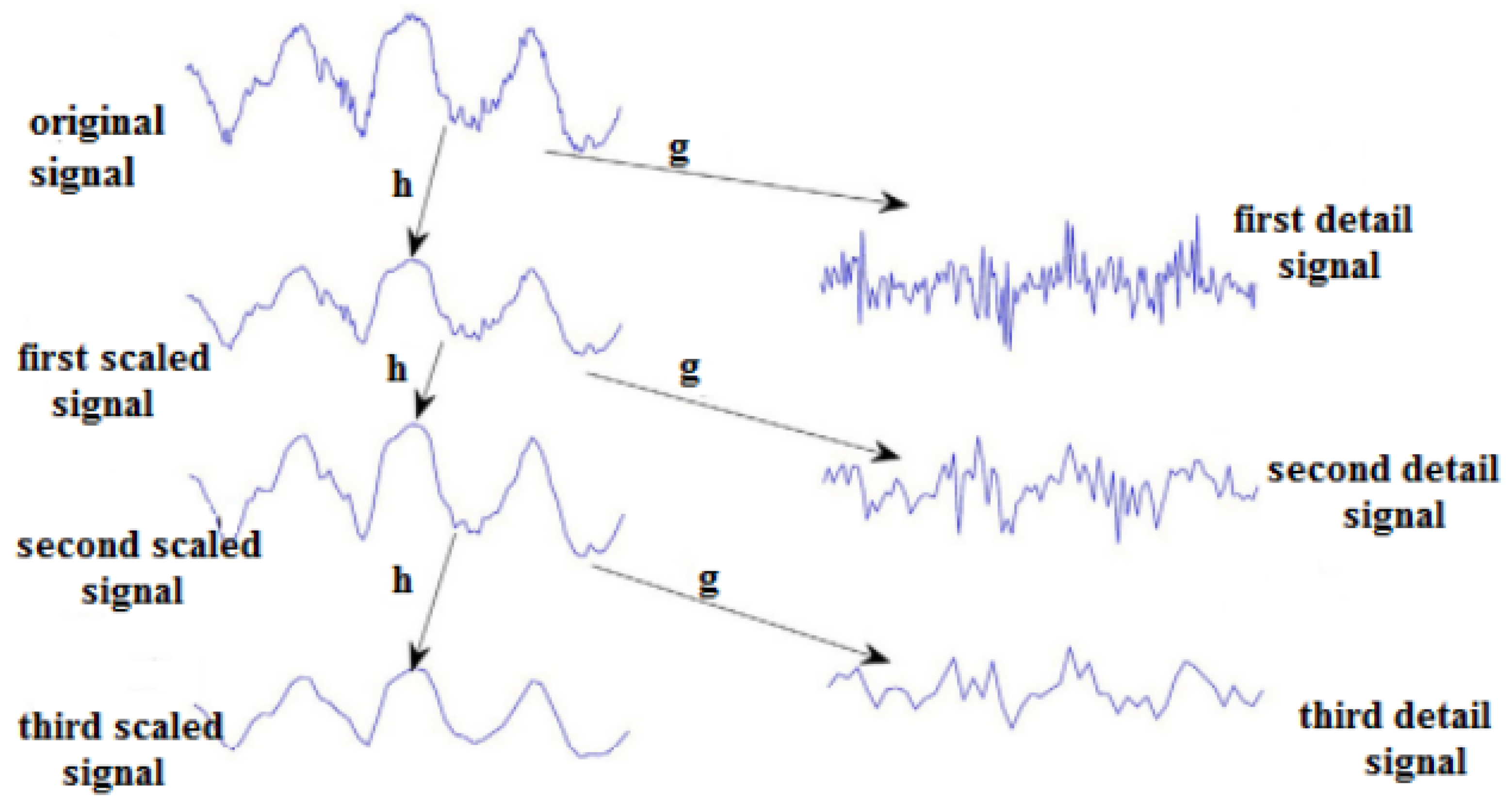
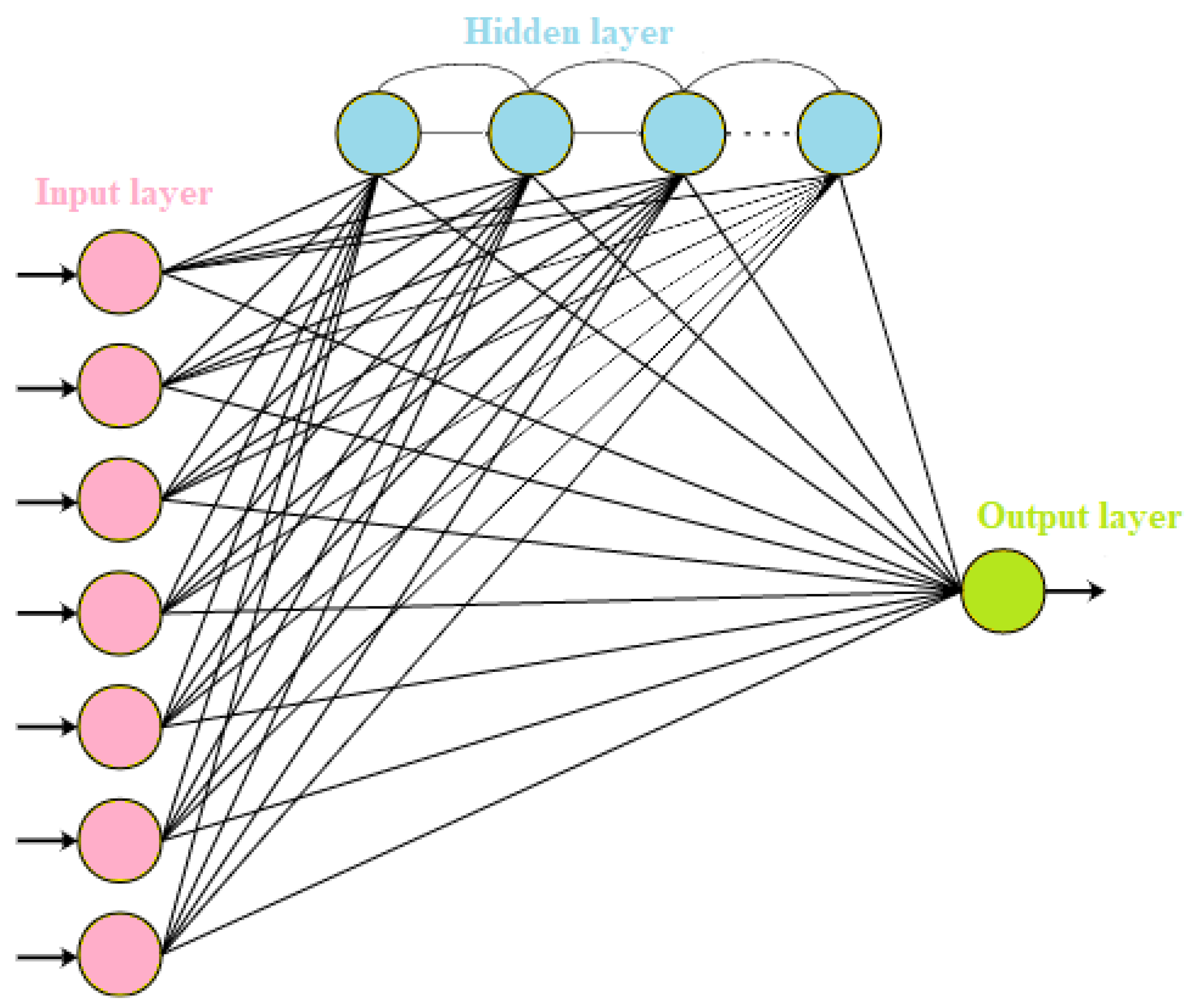
The current work proposes an intelligent fault detection/diagnosis strategy based on Multiscale Principal Component Analysis (MSPCA) and NN classifiers in order to enhance the efficiency of conventional data-driven strategies for monitoring multivariate dynamic systems. Different from the classical and standard diagnosis approaches, the proposed MSPCA-based NN approaches are used to detect and thereby isolate faults. Therefore, the contributions of this work involve three major steps: First, the data are pre-processed by the use of a multiscale scheme in order to remove noise and stochastic observations. Second, the new dataset is fed as input to a PCA method in order to extract and select the most-significant attributes from the GCPV systems in order to improve and accelerate, thereby enhance, model convergence and classification performance and accuracy. After that, the extracted features are fed as inputs to the NN classifiers in order to detect, classify, and distinguish between the different conditions. Additionally, this study is being investigated and established to address and treat all the frequent and potential faults that might occur, damage, and affect PV systems. A total of 21 fault scenarios: line-to-line, line-to-ground, connectivity, and faults that can affect the bay-pass diodes’ normal operation are introduced at various levels and locations; each scenario contains a variety of conditions, including simple faults in the $P{V}_1$ array, simple faults in the $P{V}_2$ array, multiple faults in the $P{V}_1$ array, multiple faults in the $P{V}_2$ array, and mixed faults. Various ML techniques, including Decision Tree (DT), Support Vector Machine (SVM), Discriminant Analysis (DA), k-nearest neighbor (KNN), and Naive Bayes (NB), are employed to test and evaluate the performance of our suggested strategy in terms of diagnostic precision, recall, accuracy, and computation time. The obtained results demonstrate that the evolved strategy not only improves the accuracy compared to conventional ML methods but also provides an efficient reduction in computation time and storage space.

The sections of this paper are organized and arranged as follows: A thorough explanation and detailed description of the suggested multiscale PCA-based NNs is provided in Section 2. The essential and main outcomes are presented in Section 3. The paper is concluded in Section 4.

2. Developed Multiscale PCA-Based NN

2.1. Feature Extraction Using PCA Technique

PCA is a multivariate statistical analysis technique. It is utilized for information extraction from data and has been employed in a wide range of disciplines. In the operation, monitoring, and control of chemical processes, it is also used to complete a number of tasks, such as data rectification, fault detection and isolation, and disturbance and fault diagnosis, due to its effectiveness in extracting abnormal changes from the information in the system. Therefore, the foundation of PCA is the projection of large amounts of multivariate data obtained from measurable process variables onto a reduced dimensional space of uncorrelated principal components [38]. Consider the data that were gathered in the form of a $X\in {\Re }^{n\times m}$ matrix from a process that was working normally with n samples of m variables, and store them in an X matrix with zero mean and unity [38].

$$X=[x_1,x_2,\dots ,x_m]\in {\Re }^{n\times m}$$

(1)

The following equation describes the linear transformation that turns the data matrix into another novel matrix called the score matrix of uncorrelated variables, $T={[t_1,t_2,\dots ,t_n]}^T\in {\Re }^{n\times m}$:

$$T=XP$$

(2)

The score matrix is T, and the loading matrix is P. The singular value decomposition (SVD), which is used to create an orthogonal transformation of X’s covariance matrix, results in P as depicted in the following equation:

$$C=\frac{1}{n-1}{X}^{T}X=P\Lambda P^T$$

(3)

The eigenvalues for the diagonal matrix $\Lambda =diag({\lambda }_1,{\lambda }_2,\dots ,{\lambda }_m)$ are arranged in decreasing order to indicate the variance ${\lambda }_1\ge {\lambda }_2\ge \dots \ge {\lambda }_m$. P and $\Lambda$ are divided into modeled and non-modeled variants (Figure 1) to diminish the dimensionality of the dataset. As a result, ${\Lambda }_l\in {\Re }^{l\times l}$ and $P_l\in {\Re }^{m\times l}$ span the first subspace, which is called principal subspace. Otherwise, ${\Lambda }_{m-l}\in {\Re }^{(m-l)\times (m-l)}$ and $P_{m-l}\in {\Re }^{m\times (m-l)}$ span the residual subspace (second subspace). Numerous methods, such as parallel analysis, cumulative percent variance (CPV), scree plot, kaiser criterion, and cross-validation, are used in the literature to choose principal components (PCs), l. The CPV criterion is used in the current paper in order to select the PCs, and it is depicted as the following equation:

$$CPV\left(l\right)=100\left(\frac{{\displaystyle \sum _{j=1}^l}{\lambda }_j}{{\displaystyle \sum _{j=1}^{j=m}}{\lambda }_j}\right)\%$$

(4)

2.2. Feature Selection Using PCA Technique

To obtain and accomplish high classification performance, it is essential to extract the statistical attributes using a PCA model by exhaustively listing specific available values. The two distinct indices $T^2$ and Q can be used to characterize the PCA model. Based on the first l PCs terminated for each attribute, $T^2$ determines the variations in the first subspace and the distance of each observation from the model’s center. The $T^2$ index is determined by:

$$T^2=X^T\widehat{P}\widehat{\Lambda }{\widehat{P}}^{T}X$$

(5)

The Square Predict Error (SPE), also called the Q statistic, calculates how good the PCA model is, as well as how the sampled dataset vector is projected into the second subspace [38]. Q is provided by:

$$Q=∥\tilde{X}∥={∥\left(I-\widehat{P}{\widehat{P}}^T\right)∥}^2$$

(6)

The control limits are determined for any monitoring index by the following equation:

$$T_{\alpha }^2=\frac{a(n-1)(n+1)}{n(n-a)}F\alpha (a,n-a)$$

(7)

$$Q_{\alpha }={\theta }_1{(\frac{\sqrt[c_{\alpha }]{2{\theta }_2{h}_0^2}}{{\theta }_1}+1+\frac{{\theta }_2{h}_0(h_0-1)}{{\theta }_1^2})}^{\frac{1}{h_0}}$$

(8)

$F_{\alpha }(a,n-a)$ is an evaluation of an F distribution with $a,n-a$ degrees of freedom at a specified level of confidence $(1-\alpha )$, where n is the number of samples and a is the number of PCs.

$${\theta }_i=\sum _{j=a+1}^m{\lambda }_j^i{\theta }_i=\sum _{j=a+1}^m{\lambda }_j^i,i=1,2,3$$

(9)

$$h_0=1-\frac{2{\theta }_1{\theta }_2}{3{\theta }_2^2}$$

(10)

The $(1-\alpha )$ percentile’s associated normal deviation is $c_{\alpha }$. The statistic that combines the advantages of Q and $T^2$ is depicted as:

$$\Phi =\frac{T^2}{T_{\alpha }}+\frac{Q}{Q_{\alpha }}$$

(11)

2.3. Overview of the Multiscale Representation Framework

Practical measurements are generally affected by unwanted noise, autocorrelation, and errors that conceal important elements in the dataset and restraint the efficiency of each process monitoring tool. This is because of the various physical limitations of acquisition systems. Therefore, it is necessary to first reduce the undesirable noise in order to prevent making bad decisions based on these noisy signals. In order to effectively split the stochastic features from the dataset and reduce the impacts of noise and outliers, a robust data analysis method that effectively separates deterministic and stochastic features is wavelet-based multiscale representation [39]. A low-pass filter (h), that is formed from a scaling basis function of the following form, can be used to combine a time domain data set (signal) with a low-pass filter to obtain a coarser estimation of the signal (referred to as a scaled signal), as shown in Figure 2.

$${\Phi }_{ij}\left(t\right)=\sqrt{2^{-j}}\varphi \left(2^{-j}t-k\right)$$

(12)

where k and j, respectively, stand for the discretized translation and dilation parameters. The diversity between the original and approximate signals may extracted by mixing the original signal with the use of a high-pass filter (g) (Figure 2), which is made from a wavelet basis function: [40].

$${\psi }_{ij}\left(t\right)=\sqrt{2^{-j}}\psi \left(2^{-j}t-k\right)$$

(13)

The original signal could be presented as the sum of almost recent scaled signal and all the detail signals after repeating these approximations, i.e., [40]:

$$\left[X\right]\left(t\right)=\sum _{k=1}^{n{2}^{-j}}{a}_{jk}{\varphi }_{jk}\left(t\right)+\sum _{j=1}^j\sum _{k=1}^{n{2}^{-j}}{d}_{jk}{\psi }_{jk}\left(t\right)$$

(14)

where n and j stand for the signal’s length and the highest possible decomposition, respectively. This multiscale representation process is schematically depicted in Figure 2.

$$\Phi =\frac{T^2}{T_{\alpha }}+\frac{Q}{Q_{\alpha }}$$

(15)

2.4. NNs-Based Fault Classification

For the sake of diagnosing frequent and similar faults, NN classifiers are applied to the features after noise removal, extraction, and selection of the most significant and informative attributes from the dataset. A brief review of these classifiers is given.

2.4.1. Artificial Neural Network

An organism’s nervous system, which is made up of several neurons connected in order to process data. Similar to human brains, ANN models may acquire knowledge through training, store it, and use it to estimate previously unobserved datasets [41]. The most popular ANN model is the artificial multilayer perceptron (MLP) NN. A general MLP net is an n layer NN $(n\ge 2)$. The MLP’s design generally comprises three levels: input, hidden, and output layers, as depicted in Figure 3. Therefore, gradient descent or conjugate gradient techniques are frequently used to back-propagate errors between targets, or desired values, and network outputs when training MLP [42,43].

2.4.2. Multilayer Neural Network

Three layers—input, hidden, and output—constitute the Multilayer Neural Network (MNN), as depicted in Figure 4.

Each layer is built of a set of nodes and weights that connect them. The goal of learning is to achieve the desired input/output characteristics. A back-propagation algorithm, which represents a kind of steepest descent technique, is utilized to learn an MNN by adjusting the weights. The main function that was used to train the NN is depicted in detail in [44,45].

2.4.3. Cascade Forward Neural Network (CFNN)

The CFNN algorithm is a static NN in which signals can only pass in a forward direction. Despite the fact that it connects the input and each previous layer to the subsequent ones. Indeed, the reason this network is referred to as a cascade is that all of the neurons’ output previously existed in the network and were used to feed a new neuron. When novel neurons are added to the hidden layers, the learning method tries and aims to achieve maximum correlation between the output of the added neuron and the network’s residual error, which we are seeking to low and decrease. The output layer is directly connected to an input and hidden layers in a three-layer network. Therefore, this NN has the advantage of accommodating nonlinear relationships without avoiding the linear relationship between the input and the output [46,47]. CFNN’s architecture with one hidden layer is shown in Figure 5.

2.5. MSPCA-Based NN Fault Diagnosis

In this study, the MSPCA model was applied with the goal of merging the PCA’s capacity to extract the corresponding cross-correlation betwixt variables with the orthonormal wavelets’ capacity to split features from noise and avoid the auto-correlation between the obtainable measurements. In order to combine the outcomes at adequate scales, the MSPCA technique processes and computes a PCA model of the wavelet coefficients at each scale. Accordingly, the pertinent attributes are attained for each scenario by selecting only those latent variables that capture the relationship betwixt the variables after the elimination of less important signal features. Thus, for the purpose of fault diagnosis, the most pertinent features are fed into NN classifiers. A wavelet decomposition is utilized to remove errors, decrease noise, and decorrelate the relationship between the stochastic measurements, once measurements representing healthy and various potential defective operating modes in the process are provided. The data gathered while the system is in normal operation is then used to develop a PCA model. The obtained dataset is projected onto a subspace of positive right directions while maintaining the information about the most collected features. The resultant PCA model’s structure is described by the directions of the subspace projector, whose dimension is smaller than that of the raw dataset. With the use of this projection technique, various important attributes are gathered for each situation. Subsequently, a bank of various classifiers is trained using a range of attributes as input and their associated labels as the desired output. Otherwise, a comparison between the resulting classifier output and the set of feature labels is evaluated in order to generate an efficient decision.

The main various tasks of the suggested strategy are illustrated in Figure 6.

Algorithm 1 highlights the key tasks of the MSPCA-based NN algorithm.

Algorithm 1 MSPCA-based NN algorithm

Input: $n\times m$ data matrix X,

Collecting the data.

Training phase

1. Calculate the wavelet decomposition for each column in the data matrix;

2. Calculate the mean and standard deviation of each process variable, then standardize the dataset matrix;

3. Decompose each variable into wavelet coefficients;

- Each scale’s wavelet coefficients are formed into a matrix;

- Each of these scales is subjected to PCA;

- Determine the Q, $T^2$, and $\varphi$ statistics of each dataset;

4. Retained wavelet scales and coefficients are used to reconstruct the dataset matrix;

5. Perform PCA to acquire an estimated dataset matrix and residuals;

6. Classify the faults through NN classifiers;

7. Ascertain the classification model;

Testing phase

1. Standardize the testing dataset by the use of the mean and the standard deviation computed from the fault-free training phase;

2. Decompose each variable into wavelet coefficients;

- Each scale’s wavelet coefficients are formed into a matrix;

- Each of these scales is subjected to PCA;

- Determine the Q, $T^2$, and $\varphi$ statistics of each dataset;

3. Reconstruct the data matrix by use of the retained wavelet scales and coefficients;

4. A PCA technique is performed on the reconstructed data matrix;

5. Classify the faults through NN classifiers;

6. Establish the prediction model;

7. Attain the fault diagnosis outcomes.

3. Results and Discussion

3.1. Process Description

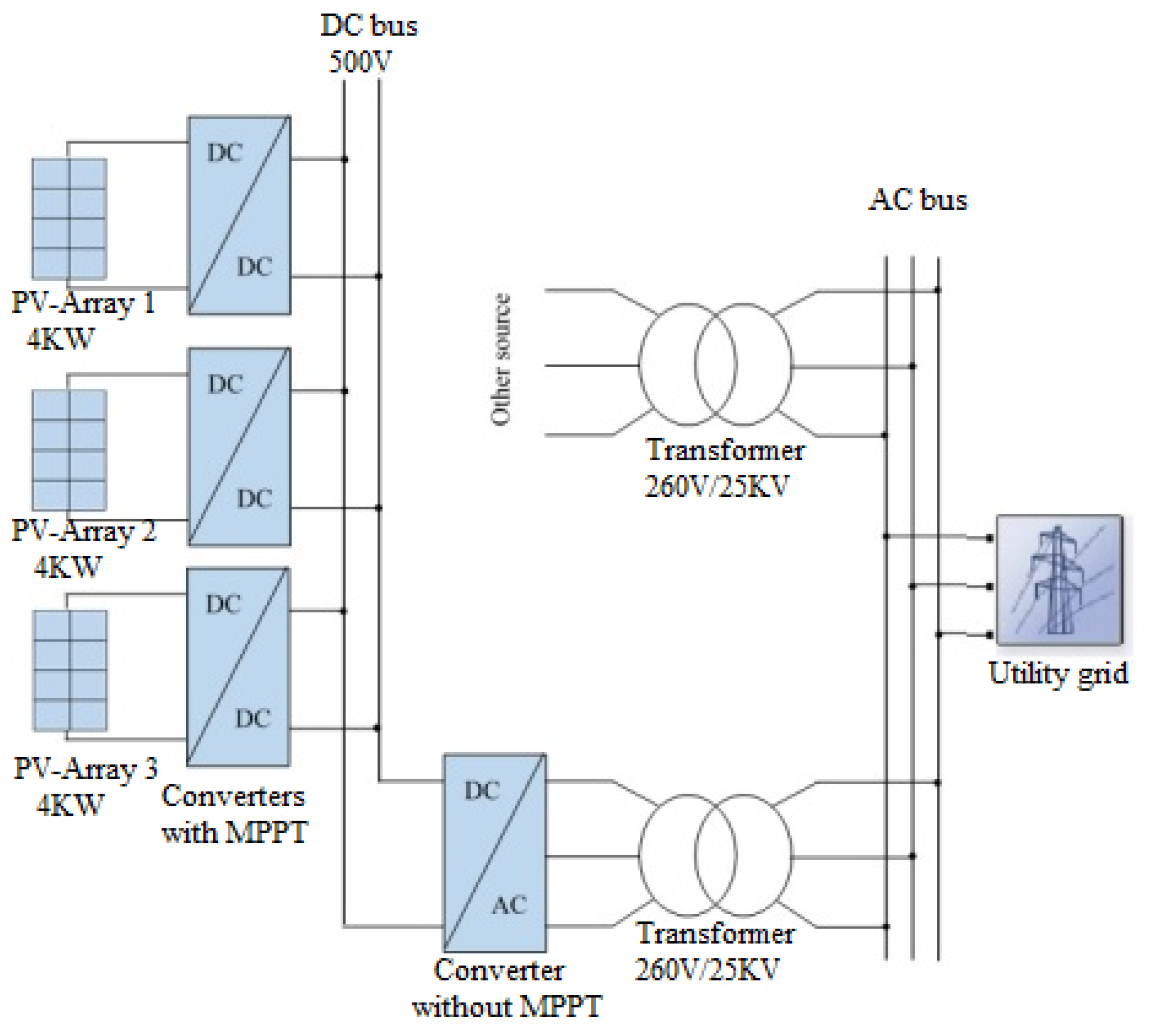
In this work, the distributed structure has been considered. This structure is a modular application that allows the multiplication and diversification of technologies, for which the combination of several different types of photovoltaic sensors can be made. One aspect of the possible configuration is shown in Figure 7. A DC voltage bus with a 500-volt value is involved. All panel and converter components are linked in parallel to the DC voltage bus. Because each panel is optimally controlled individually, the downstream converter does not control the global MPP tracking. Besides, the controllers are resistant to external perturbations. Because of the used high voltage, it is possible to consider a reduction of the cable sections, which constitutes a material gain in copper or aluminum. The PV farm consists of 3 PV arrays, each delivering a maximum of 4 kW. A single PV array block is made up of two parallel strings, each having 24 modules connected in series. In each module, there are 20 cells. Each PV array has a DC/DC converter connected to it. The outputs of the boost converters are connected to a common 500-volt DC bus. Each boost is individually controlled using Maximum PowerPoint Trackers (MPPT). The PV array’s terminal voltage is varied by the MPPTs using the “perturb and observe” technique in order to obtain the maximum possible power. A three-phase source converter transforms the 500 V DC to 260 V AC and keeps the unity power factor. To connect the converter to the grid, a 100 (kVA) 260 (V)/25 (kV) three-phase coupling transformer is employed.

3.2. Description of the Input Data

Twenty-one frequent PV faults ($Faul{t}_1$, $Faul{t}_2$…, $Faul{t}_{21}$) are treated in this current work.

As shown in

Table 1. Detailed description of the diverse injected labeled faults.

Type of Fault	Fault Label	Fault Description
Simple faults in $P{V}_1$	$Faul{t}_1$	Line-to-Line fault (LL1)
	$Faul{t}_2$	Line-to-Ground fault (LG1)
	$Faul{t}_3$	Connectivity fault (Cn1)
	$Faul{t}_4$	Bypass fault (BP1)
Simple faults in $P{V}_2$	$Faul{t}_5$	Line-to-Line fault (LL2)
	$Faul{t}_6$	Line-to-Ground fault (LG2)
	$Faul{t}_7$	Connectivity fault (Cn2)
	$Faul{t}_8$	Bypass fault (BP2)
Multiple faults in $P{V}_1$	$Faul{t}_{13}$	LL1 + LG1 + Cn1
Multiple faults in $P{V}_2$	$Faul{t}_{14}$	LL2 + LG2 + Cn2
Mixed faults	$Faul{t}_9$	LL1 + LG1 + LL2
	$Faul{t}_{10}$	Cn1 + LL2+ LG2
	$Faul{t}_{11}$	BP1 + LL1 + BP2
	$Faul{t}_{12}$	LL2+ BP2 + LG2
	$Faul{t}_{15}$	BP1 + BP2
	$Faul{t}_{16}$	LL1 + LL2
	$Faul{t}_{17}$	LG1 + LG2
	$Faul{t}_{18}$	Cn1 + Cn2
	$Faul{t}_{19}$	LL1 + LG2
	$Faul{t}_{20}$	LG1 + LL2
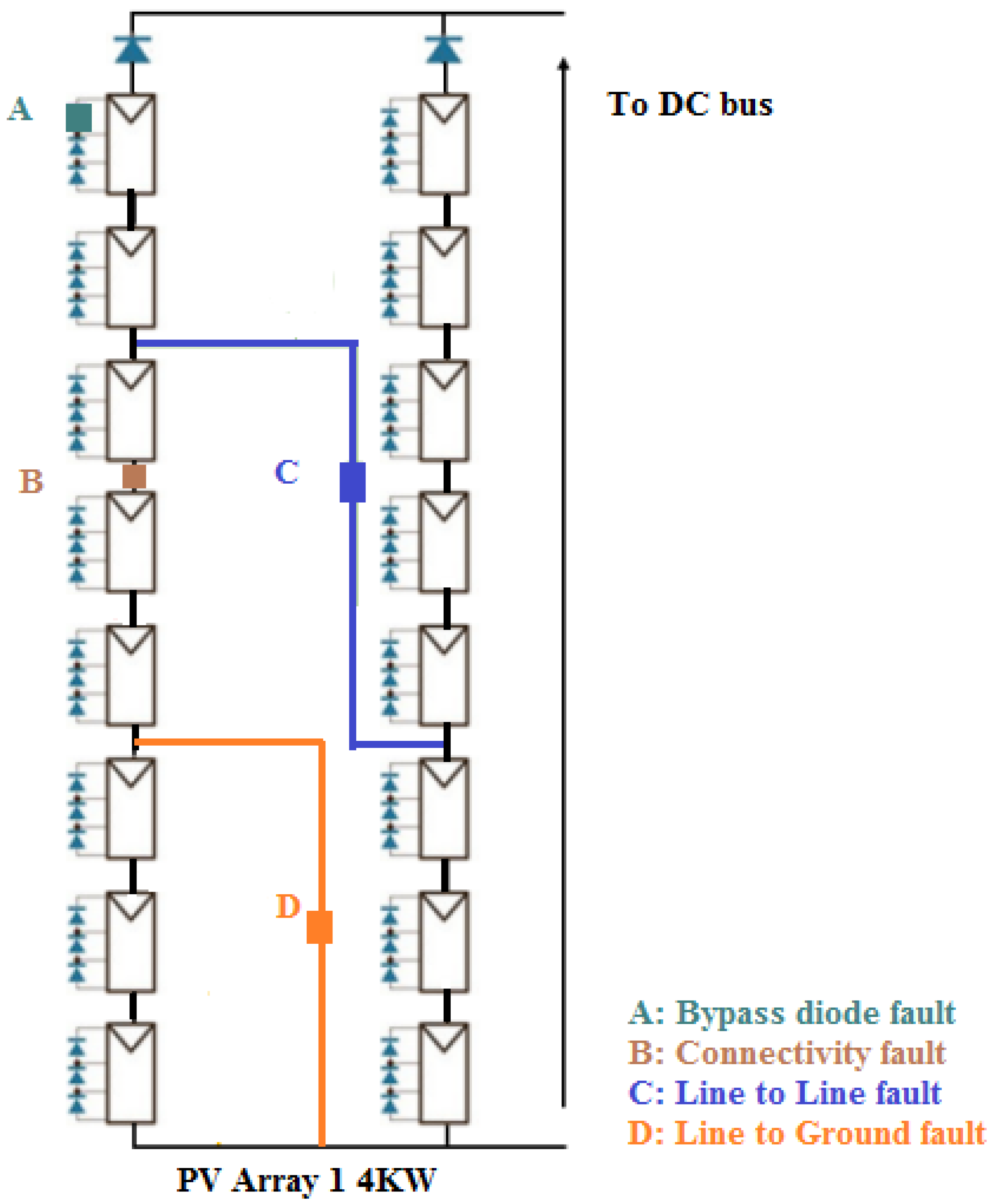
	$Faul{t}_{21}$	Cn1 + BP2

, we used five different types of faults to introduce various scenarios into the $P{V}_1$ and $P{V}_2$ systems in this work; for example, PV1’s simple faults include four possible fault scenarios: $Faul{t}_1$ (line-to-line fault) is injected betwixt two distinct points; a line-to-ground fault ($Faul{t}_2$) is considered in String1 ($St{r}_1$) positioned betwixt one point and the ground; $Faul{t}_3$ (connectivity fault) is injected in the first string between two modules; $Faul{t}_4$ impacts the bay-pass diodes by injecting a variation in resistance, the diverse positions of the aforementioned failures are shown in Figure 8.

The second PV array receives the same simple fault injections. Then, numerous defects that present multiple faults are introduced into one PV array ($P{V}_1$ or $P{V}_2$). In addition, we simultaneously injected mixed faults, which reflect numerous faults in both PV arrays.

The used simulated variables, which are gathered in order to assess FDD performance, are presented in [48].

3.3. Fault Classification Results

The investigated GCPV system operates in 22 working modes (Class $C_i,i=0...21$) when the first mode is the healthy one. A sample training dataset using 50 percent of the data was utilized in order to train the NNs, and the remaining data were utilized to validate and evaluate the trained NNs (see

Table 2. Construction of the database.

Type of Fault	Class	State	Training Dataset	Testing Dataset
Fault-free	$C_0$	healthy case	3000	3000
Simple faults in $P{V}_1$	$C_1$	$Faul{t}_1$	3000	3000
	$C_2$	$Faul{t}_2$	3000	3000
	$C_3$	$Faul{t}_3$	3000	3000
	$C_4$	$Faul{t}_4$	3000	3000
Simple faults in $P{V}_2$	$C_5$	$Faul{t}_5$	3000	3000
	$C_6$	$Faul{t}_6$	3000	3000
	$C_7$	$Faul{t}_7$	3000	3000
	$C_8$	$Faul{t}_8$	3000	3000
Multiple faults in $P{V}_1$	$C_{13}$	$Faul{t}_{13}$	3000	3000
Multiple faults in $P{V}_2$	$C_{14}$	$Faul{t}_{14}$	3000	3000
Mixed faults	$C_9$	$Faul{t}_9$	3000	3000
	$C_{10}$	$Faul{t}_{10}$	3000	3000
	$C_{11}$	$Faul{t}_{11}$	3000	3000
	$C_{12}$	$Faul{t}_{12}$	3000	3000
	$C_{15}$	$Faul{t}_{15}$	3000	3000
	$C_{16}$	$Faul{t}_{16}$	3000	3000
	$C_{17}$	$Faul{t}_{17}$	3000	3000
	$C_{18}$	$Faul{t}_{18}$	3000	3000
	$C_{19}$	$Faul{t}_{19}$	3000	3000
	$C_{20}$	$Faul{t}_{20}$	3000	3000
	$C_{21}$	$Faul{t}_{21}$	3000	3000

).

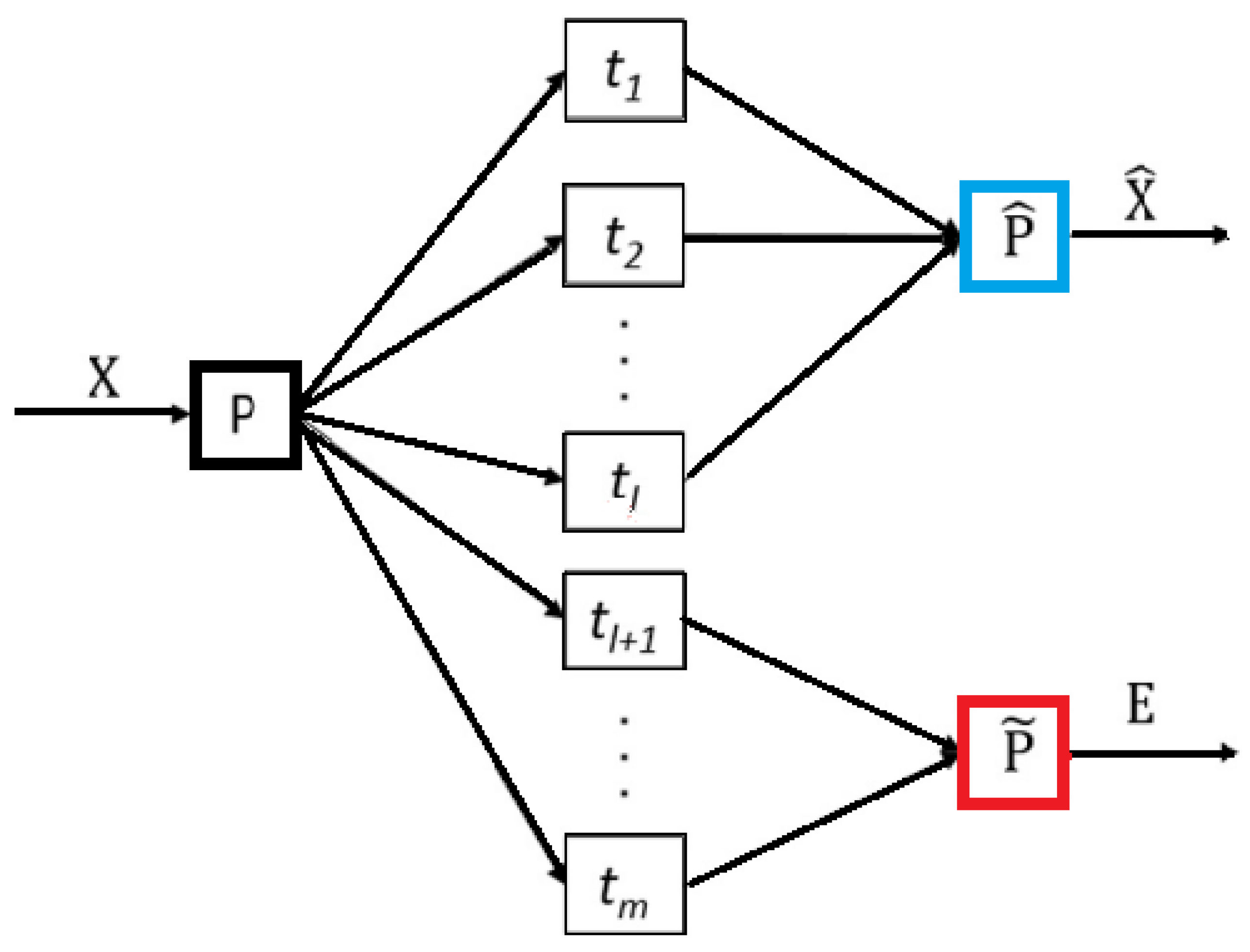
In the present work, a method for detecting and diagnosing faults is provided. Almost all stochastic measurements are decor-related. After being normalized to have unit variance and zero mean, a PCA model is generated. Then, using a 95% cumulative variance criterion, the acquired variances of the variables are stored and arranged in decreasing order after being computed by the use of the eigenvalue decomposition. Consequently, five PCs were maintained to be utilized to train the NN classifiers.

Therefore, denoising variables and selecting and thereby extracting statistical features using an MSPCA tool is crucial for achieving higher accuracy in FDD-based techniques. As a result, in this study, the NN classifiers are introduced with the newly obtained dataset. Using labeled training data, this method teaches a set of predefined fault types.

Several ML techniques, including DT, SVM, DA, KNN, and NB, are employed to test and evaluate the performance of our suggested strategy in terms of diagnostic precision, recall, accuracy, and computation time.

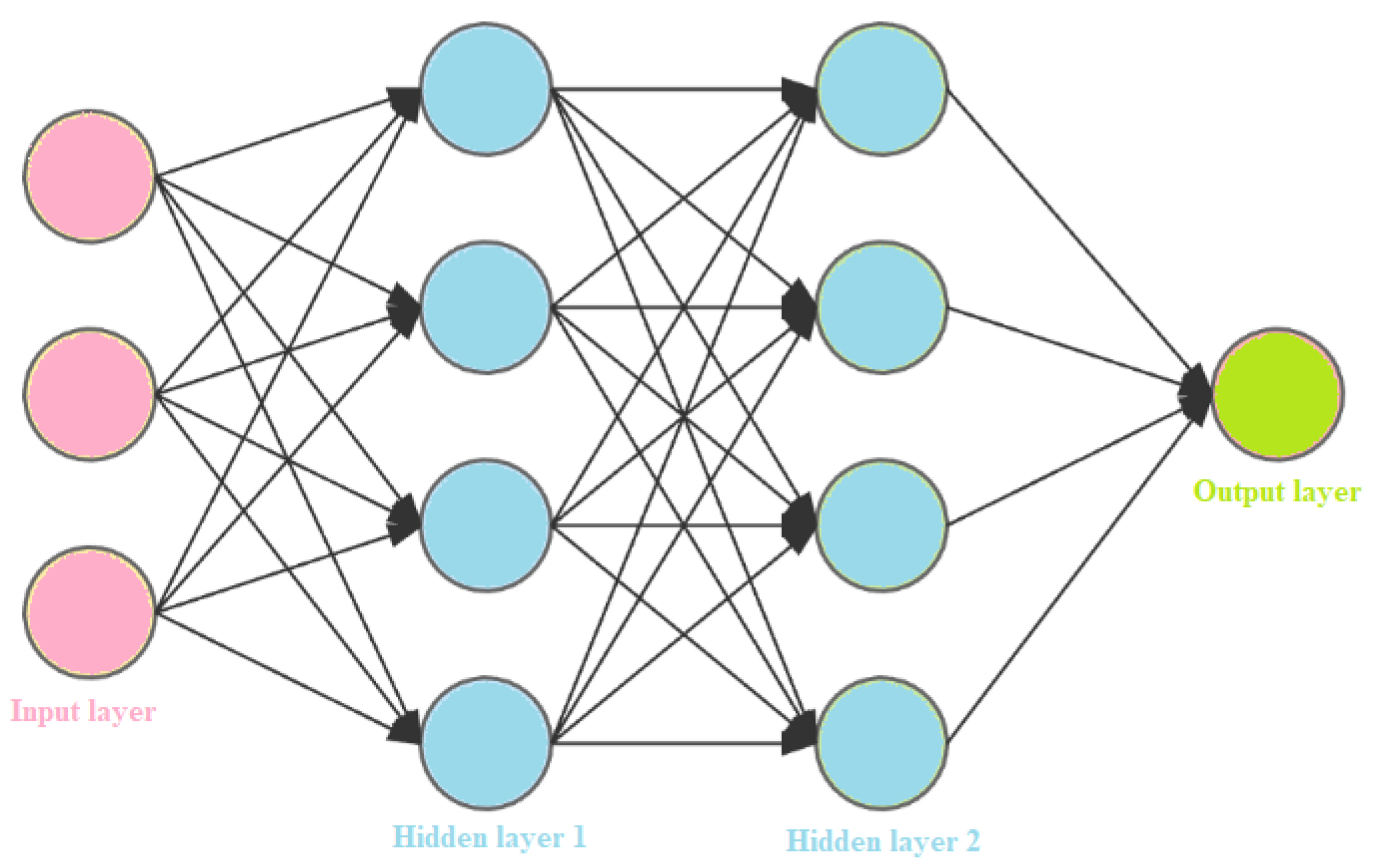
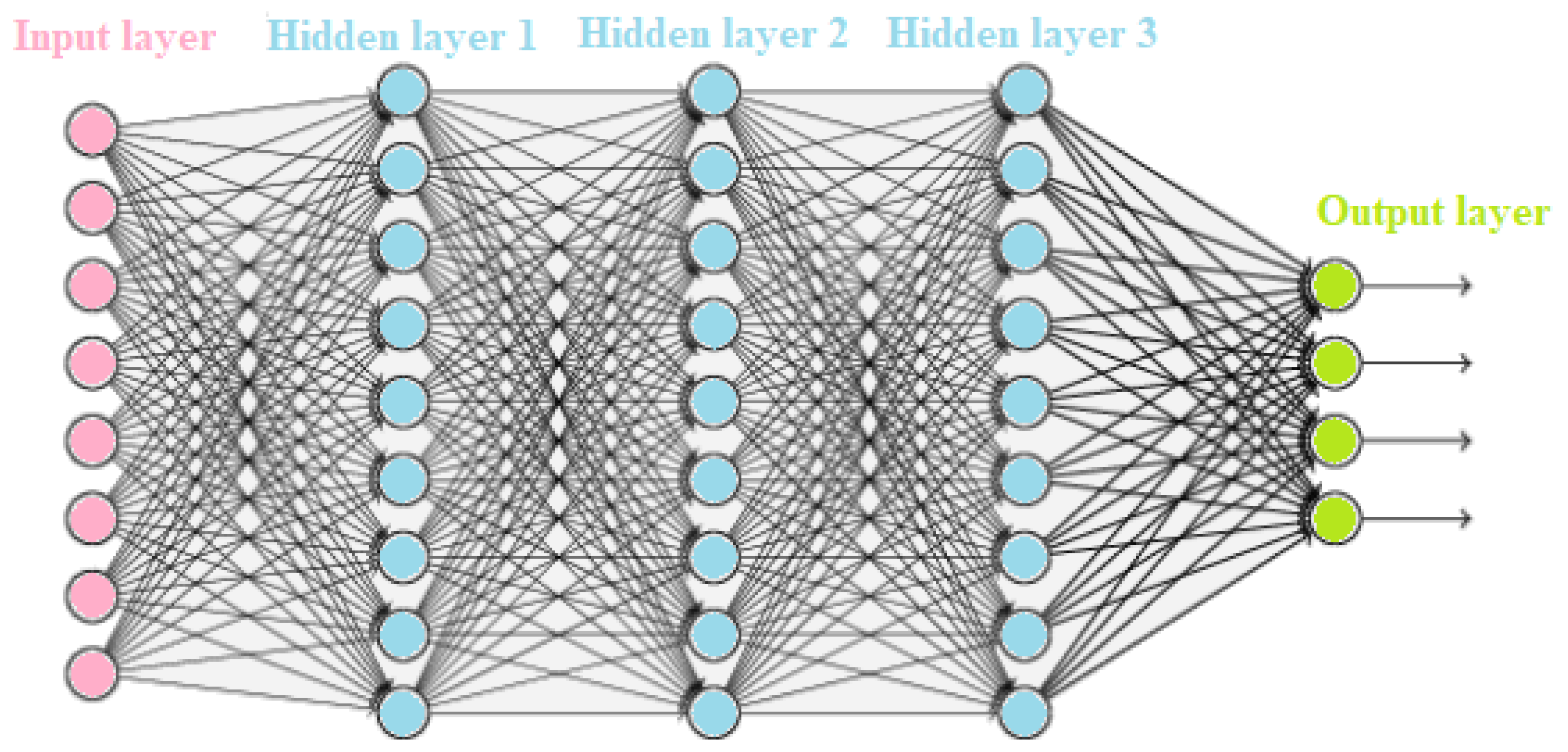
The different existing techniques are implemented in a MATLAB environment. The accuracy of these techniques is computed using a 10-fold cross-validation metric in order to determine the FDD efficiency of the suggested techniques. The number of hidden layers selected for the NN and CFNN is 10, and it was [10, 10, 10] for MNN, with a total of 50 max epochs with full batch size. The K value for KNN is equal to 3, and the K and C parameters for SVM are set with the lowest RMSE value. The number of splits for DT is equal to 50.

This work then employs a PCA model with a $\left\{P{C}_{l=5},Q,\Phi \right\}$ group of features.

Table 3. Normalized accuracy for the various extracted features and the NN classifiers.

Classifiers	Phase	Normalized Accuracy	CT (s)
ANN	Training	0.8249	88.23
	Testing	0.9166	0.62
MNN	Training	0.6486	110.98
	Testing	0.8220	0.68
CFNN	Training	0.6611	4260.8
	Testing	0.6674	0.40
DT	Training	0.7364	23.18
	Testing	0.7349	0.20
SVM	Training	0.8569	3700.79
	Testing	0.8532	500.31
KNN	Training	0.8157	5.57
	Testing	0.8212	0.82
NB	Training	0.2143	5.75
	Testing	0.2368	0.50
DA	Training	0.3744	4.92
	Testing	0.3721	0.46

shows the overall normalized accuracy values for the various extracted features and the NN classifiers.

Table 4. MSPCA normalized accuracy values for the diverse extracted features and NN classifiers.

Classifiers	Phase	MSPCA Normalized Accuracy	CT (s)
ANN	Training	0.9149	72.26
	Testing	0.9363	0.45
MNN	Training	0.8461	118.4
	Testing	0.9419	0.65
CFNN	Training	0.8359	4195.8
	Testing	0.8362	0.53
DT	Training	0.8436	11.90
	Testing	0.8634	0.093
SVM	Training	0.8911	2125.14
	Testing	0.8660	218.26
KNN	Training	0.8722	3.60
	Testing	0.8235	0.40
NB	Training	0.7262	3.27
	Testing	0.7259	0.25
DA	Training	0.4383	2.86
	Testing	0.4317	0.21

shows the obtained results in terms of normalized accuracy values for the diverse extracted features based on the combined MSPCA technique and the NN classifiers.

The established MSPCA-based NN methods are demonstrated to be efficient alternatives for fault diagnosis when compared to other existing methods. In spite of the fact that the MSPCA tool enhances and improves the overall performance of all the utilized techniques, the conventional methods still have significant drawbacks. For instance, the accuracy of the DA and NB approaches is still poor, and the SVM technique suffers from a difficult training phase and a high time complexity. In effect, it is clear that the suggested approach performs better and produces good outcomes in terms of classification accuracy compared to conventional techniques.Indeed, the accuracy of the training and testing phases of the ANN classifier increased by 9 and 1.97 percent, respectively, the training and testing phase accuracy of the MNN classifier improved by 19.75 and 11.99 percent, respectively; and indeed, for the CFNN classifier, the training mode accuracy increased by 17.48 percent and the testing mode accuracy by 16.88 percent. Besides, the evolved strategy reduces and decreases the computation time (CT), which speeds up the NN classifiers and slows down their convergence. For instance, for the ANN classifier, the CT has been decreased by 15.97 (s) and 0.17 (s) for the training and testing phases, respectively.

Table 5. Normalized confusion matrix of ANN classifier on testing phase.

	True Classes
Predicted Classes	${\mathit{C}}_0$	${\mathit{C}}_1$	${\mathit{C}}_2$	${\mathit{C}}_3$	${\mathit{C}}_4$	${\mathit{C}}_5$	${\mathit{C}}_6$	${\mathit{C}}_7$	${\mathit{C}}_8$	${\mathit{C}}_9$	${\mathit{C}}_{10}$	${\mathit{C}}_{11}$	${\mathit{C}}_{12}$	${\mathit{C}}_{13}$	${\mathit{C}}_{14}$	${\mathit{C}}_{15}$	${\mathit{C}}_{16}$	${\mathit{C}}_{17}$	${\mathit{C}}_{18}$	${\mathit{C}}_{19}$	${\mathit{C}}_{20}$	${\mathit{C}}_{21}$	Normalized Precision
$C_0^{\prime }$	28.09	0	0	0	1.56	0	0	0	0.43	0	0	0	0	0	0	0.79	0.30	1.33	0	0.41	0	0	0.8535
$C_1^{\prime }$	0.09	28.63	0	0	0	0	0	0	0	0.46	0	1.20	0	0	0	0	0	0	0	0	0	0.06	94.05
$C_2^{\prime }$	0	1.04	29.60	0.21	0	0	0	0	0	0.49	0	0	0	0	0	0	0	0	0	0	0	0	0.9444
$C_3^{\prime }$	0.26	0.32	0.04	28.58	0	0	0	0	0	0.10	0	0	0	0	0	0	0	0	0	0	0	2.45	0.9001
$C_4^{\prime }$	0	0	0	0.16	27.55	0	0	0	0	0	0	0	0	0	0	0.02	0	0.09	0	0	0	0	0.9902
$C_5^{\prime }$	0	0	0	0	0	29.44	0.38	0.53	0	0	0.48	0	0	0	0	0	0	0	0	0	0	0	0.9549
$C_6^{\prime }$	0	0	0	0	0	0	27.96	0	0.67	0	0.61	0	0	0.01	0.28	0	0	0	0	0	0	0	0.9471
$C_7^{\prime }$	0	0	0	0	0	0.25	0.32	29.21	0	0	0.08	0	0	0	0	0	0	0	0	0.10	0.01	0	0.9746
$C_8^{\prime }$	0.01	0	0	0	0.56	0	0	0.05	28.20	0	0	0.31	0	0	0	0.97	0	0	0	0	0.23	0	0.9297
$C_9^{\prime }$	0	0.01	0.24	0.97	0	0	0	0	0	28.73	0	0	0	0.11	0	0	0	0	0	0	0.15	0.27	0.9425
$C_{10}^{\prime }$	0	0	0	0	0.11	0.31	1.02	0	0	0	28.21	0.37	0.46	0	0.28	0	0	0	0	0	0	0	0.9171
$C_{11}^{\prime }$	0	0	0	0	0	0	0	0	0	0	0	27.21	0	0.18	0	0.26	0	0	0	0	0	0	0.9840
$C_{12}^{\prime }$	0	0	0	0	0	0	0.24	0.21	0	0	0.10	0	25.78	0.03	6.56	0	0	0	0	0	0	0	0.7831
$C_{13}^{\prime }$	0	0	0	0.08	0	0	0	0	0	0	0	0	0	29.59	0	0	0	0	0	0	6	0	0.9952
$C_{14}^{\prime }$	0	0	0	0	0	0	0.06	0	0	0	0.25	0.15	3.57	0	22.88	0.04	0	0	0	0	0.11	0	0.8455
$C_{15}^{\prime }$	0	0	0	0	0.19	0	0	0	0	0	0	0.10	0	0	0	27.51	0.10	0.69	0.21	0	0.03	0	0.9542
$C_{16}^{\prime }$	0	0	0	0	0	0	0	0	0	0	0	0	0	0	0	0	29.32	0.30	0.81	0	0	0	0.9635
$C_{17}^{\prime }$	0	0	0	0	0	0	0	0	0	0	0	0	0	0	0	0.12	0.17	27.58	0.82	0.17	0	0	0.9556
$C_{18}^{\prime }$	1.47	0	0	0	0	0	0	0	0	0	0	0	0	0	0	0.02	0.11	0.01	28.16	0	0	0	0.9459
$C_{19}^{\prime }$	0.08	0	0.12	0	0	0	0	0	0	0	0	0.07	0.01	0	0	0.27	0	0	0	29.29	0.19	0	0.9753
$C_{20}^{\prime }$	0	0	0	0	0.03	0	0.02	0	0	0.06	0.27	0	0.01	0.08	0	0	0	0	0	0.03	29.22	0	0.9831
$C_{21}^{\prime }$	0	0	0	0	0	0	0	0	0.70	0.16	0	0.59	0	0.08	0	0	0	0	0	0	0	27.22	0.9467
Normalized recall	0.9363	0.9543	0.9866	0.9526	0.9183	0.9813	0.932	0.9736	0.94	0.9576	0.9403	0.9007	0.8593	0.9863	0.7626	0.917	0.9773	0.9193	0.9386	0.9763	0.974	0.9073	0.9363

,

Table 6. Normalized confusion matrix of MNN classifier on testing phase.

	True Classes
Predicted Classes	${\mathit{C}}_0$	${\mathit{C}}_1$	${\mathit{C}}_2$	${\mathit{C}}_3$	${\mathit{C}}_4$	${\mathit{C}}_5$	${\mathit{C}}_6$	${\mathit{C}}_7$	${\mathit{C}}_8$	${\mathit{C}}_9$	${\mathit{C}}_{10}$	${\mathit{C}}_{11}$	${\mathit{C}}_{12}$	${\mathit{C}}_{13}$	${\mathit{C}}_{14}$	${\mathit{C}}_{15}$	${\mathit{C}}_{16}$	${\mathit{C}}_{17}$	${\mathit{C}}_{18}$	${\mathit{C}}_{19}$	${\mathit{C}}_{20}$	${\mathit{C}}_{21}$	Normalized Precision
$C_0^{\prime }$	27.29	0	0	0	0.57	0	0	0	1.83	0	0	0	0	0	0	1.21	0.29	0.41	0.44	0	0	0	0.8517
$C_1^{\prime }$	0	28.54	0	0.01	0	0	0	0	0	0	0	1.02	0	0	0	0	0	0	0	0	0	0	0.9651
$C_2^{\prime }$	0	0.27	29.52	0	0	0	0	0	0	0	0	0	0	0	0	0	0	0	0	0	0.08	0.05	0.9866
$C_3^{\prime }$	0	0	0.20	29.50	0	0	0	0	0	1.61	0	0	0	0	0	0.20	0	0	0	0	0.04	2.35	0.8656
$C_4^{\prime }$	0.53	0	0	0.21	29.15	0	0	0	0	0	0	0	0	0	0	0.31	0	0.07	0	0	0	0	0.9629
$C_5^{\prime }$	0	0	0	0	0.02	29.14	0.50	0.40	0	0	0.23	0	0	0	0	0	0	0	0	0	0.59	0	0.9436
$C_6^{\prime }$	0	0	0	0	0	0	28.77	0.10	0	0	2.21	0	0	0	0	0	0	0	0	0	0	0	0.9256
$C_7^{\prime }$	0	0	0	0	0	0.19	0.15	27.66	0	0	0	0.05	0	0	0	0	0	0	0.14	0	0.11	0	0.9773
$C_8^{\prime }$	0.26	0	0	0	0.03	0	0	0	27.21	0	0	0	0	0	0	9.54	0	0	0	0	0.04	0	0.9690
$C_9^{\prime }$	0	0.27	0	0	0	0	0	0	0	28.18	0	0.22	0	0.17	0	0	0	0	0	0	0	0	0.9771
$C_{10}^{\prime }$	0	0	0	0	0	0.67	0.47	0.88	0	0	27.20	0.14	0.14	0	0.53	0.02	0	0	0.03	0	0	0	0.9042
$C_{11}^{\prime }$	0	0.77	0	0	0	0	0	0	0	0.06	0	28.13	0	0.21	0	0	0	0	0	0	0	0	0.9643
$C_{12}^{\prime }$	0	0	0	0	0	0	0	0	0	0	0	0	26.93	0	2.40	0	0	0	0	0	0	0	0.9181
$C_{13}^{\prime }$	0	0.06	0	0.01	0	0	0	0	0	0	0	0	0	28.92	0	0	0	0	0.08	0	0	0	0.9948
$C_{14}^{\prime }$	0	0	0	0	0	0	0.11	0	0	0.05	0.29	0.01	2.32	0	27.02	0.16	0	0.05	0	0.03	0.19	0	0.823
$C_{15}^{\prime }$	0	0	0	0	0.05	0	0	0	0	0	0.07	0.02	0	0.09	0	27.22	0	0.62	0.12	0	0.16	0	0.9601
$C_{16}^{\prime }$	0.42	0.06	0	0	0	0	0	0	0	0	0	0	0	0	0	0	29.25	0.29	0.44	0.48	0	0	0.8295
$C_{17}^{\prime }$	0.22	0	0	0	0	0	0	0	0.06	0	0	0.03	0	0	0	0	0	28.21	0.39	0.18	0	0	0.9697
$C_{18}^{\prime }$	1.28	0	0	0.10	0	0	0	0.06	0	0	0	0.02	0	0	0	0.09	0.28	0.22	28.36	0.19	0	0	0.9267
$C_{19}^{\prime }$	0	0	0	0	0	0	0	0	0	0	0	0.06	0.61	0.12	0	0.25	0.18	0.13	0	29.12	0.03	0	0.9547
$C_{20}^{\prime }$	0	0.03	0.03	0	0.18	0	0	0.90	0	0	0	0	0	0.23	0.05	0	0	0	0	0	28.76	0	0.9529
$C_{21}^{\prime }$	0	0	0.25	0.17	0	0	0	0	0.90	0.10	0	0.30	0	0.26	0	0	0	0	0	0	0	27.60	0.9330
Normalized recall	0.9096	0.9513	0.984	0.9833	0.9716	0.9713	0.959	0.922	0.907	0.9393	0.9066	0.9376	0.8976	0.964	0.9006	0.9073	0.975	0.9403	0.9453	0.9706	0.9586	0.92	0.9419

and

Table 7. Normalized confusion matrix of CFNN classifier on testing phase.

	True Classes
Predicted Classes	${\mathit{C}}_0$	${\mathit{C}}_1$	${\mathit{C}}_2$	${\mathit{C}}_3$	${\mathit{C}}_4$	${\mathit{C}}_5$	${\mathit{C}}_6$	${\mathit{C}}_7$	${\mathit{C}}_8$	${\mathit{C}}_9$	${\mathit{C}}_{10}$	${\mathit{C}}_{11}$	${\mathit{C}}_{12}$	${\mathit{C}}_{13}$	${\mathit{C}}_{14}$	${\mathit{C}}_{15}$	${\mathit{C}}_{16}$	${\mathit{C}}_{17}$	${\mathit{C}}_{18}$	${\mathit{C}}_{19}$	${\mathit{C}}_{20}$	${\mathit{C}}_{21}$	Normalized Precision
$C_0^{\prime }$	21.14	0	0	0	1.65	0	0.02	0.23	1.72	0	0	0	0	0	0	0.54	0.23	1.33	6.47	0.43	0.15	0	0.6234
$C_1^{\prime }$	0	28.74	0.08	0.45	0	0	0	0	0	2.04	0	0.66	0	0	0	0	0	0	0	3.15	0	0.60	0.8045
$C_2^{\prime }$	0.10	0.79	28.61	1.51	0	0	0	0	0	4.01	0	0.01	0	0	0	0	0	0	0	0	0.05	0.74	0.7987
$C_3^{\prime }$	1.50	0	0	26.86	0	0	0	0	0	0.07	0	0	0	0	0	0.01	0	0	0	0	0	2.01	0.8821
$C_4^{\prime }$	0.61	0	0	0.74	27.51	0	0	0	0	0	0	0	0	0	0	0.01	0	0.06	2.03	0	0.06	0	0.8868
$C_5^{\prime }$	0.18	0	0	0	0.05	29.81	1.23	0.55	0.45	0	2.11	0	0	0	0	0.37	0.38	0.75	0.26	0.25	0.71	0	0.8035
$C_6^{\prime }$	0	0	0	0	0	0	26.85	0.74	0	0	10.84	0.04	0.23	0	0.46	0.16	0	0	0	0.03	0.44	0	0.6809
$C_7^{\prime }$	0	0	0	0	0	0	1.30	28.25	0	0	2.79	0.18	0.28	0	0.01	0	0	0	0	0	2.64	0	0.7968
$C_8^{\prime }$	1.74	0	0	0	0.01	0	0	0.0 4	26.84	0	0	0.24	0	0	0	1.21	0	0.02	0	0	0.16	0	0.8869
$C_9^{\prime }$	0	0	0	0	0	0	0	0	0	20.21	0	0	0	0.11	0	0	0	0	0	0	0	0	0.9945
$C_{10}^{\prime }$	0	0	0	0	0	0	0	0	0	0	0.53	0	0.14	0	0	0	0	0	0	0	0	0	0.7910
$C_{11}^{\prime }$	0	0.11	0	0	0	0	0	0	0	0	0	28.07	0	0.72	0	0	0	0	0	5.87	0	0	0.8073
$C_{12}^{\prime }$	0	0	0	0	0	0	0	0	0	0	0.15	0	28.87	0	1.97	0	0	0	0	0	0	0	0.9315
$C_{13}^{\prime }$	0	0	0	0	0	0	0	0	0	0	0	0	0	28.97	0	0	0	0	0	0	0	0	1
$C_{14}^{\prime }$	0	0	0	0	0	0.19	0.60	0	0	0	12.37	0	0.14	0	27.23	0.06	0	0	0	0	0	0	0.6755
$C_{15}^{\prime }$	0.03	0	0	0	0.78	0	0	0	0	0	0	0	0	0	0	27.47	0.06	1.67	1.80	0	0	0	0.8635
$C_{16}^{\prime }$	0	0.22	0.81	0.24	0	0	0	0	0	0.31	0	0.31	0	0	0	0	29.22	0	0.58	0.22	0	0	0.9157
$C_{17}^{\prime }$	0	0	0	0	0	0	0	0	0	0	0.75	0.28	0	0	0	0	0	26.17	0.43	0	0	0	0.9471
$C_{18}^{\prime }$	4.70	0	0	0	0	0	0	0.19	0	0	0	0	0	0	0	0	0.08	0	18.43	0.13	0	0	0.7832
$C_{19}^{\prime }$	0	0	0.32	0	0	0	0	0	0	0	0	0	0.20	0	0	0	0	0	0	19.92	0.24	0	0.9632
$C_{20}^{\prime }$	0	0	0	0	0	0	0	0	0	3.24	0.46	0.04	0	0.03	0.33	0	0	0	0	0	25.55	0	0.8617
$C_{21}^{\prime }$	0	0.14	0.18	0.20	0	0	0	0	0.99	0.12	0	0.17	0.14	0.17	0	0.17	0.3	0	0	0	0	26.65	0.9202
Normalized recall	0.7046	0.958	0.9536	0.8953	0.917	0.9936	0.895	0.9416	0.8946	0.6736	0.0176	0.9356	0.9623	0.9656	0.9076	0.9156	0.974	0.8723	0.6143	0.664	0.8516	0.8883	0.8362

present the obtained testing classification outcomes of diverse classes by the use of the normalized confusion matrix in order to indicate the efficiency of the developed strategies. In fact, this matrix presents the samples that were correctly classified as well as the ones that were incorrectly classified for the healthy ($C_0$) and faulty modes ($C_1$ to $C_{21}$). Actual classes and predicted process statuses are indicated by the raw and the column, respectively.

Table 5 shows that for faulty operating mode 1 ($C_1$), the ANN classifier recognizes 2863 observations out of 3000 (true positive) observations. For this scenario, the detection precision is 94.05 percent, the recall is 95.43 percent, and the misclassification rate is equal to 4.57%. For $Faul{t}_2$, designated to class C2, the precision is equal to 94.44%, the recall is 98.66%, and the misclassification rate is equal to 1.34%. The Precision for $Faul{t}_3$ is 90.01%, the recall is 95.26%, and there is a 4.74% misclassification. The misclassification is therefore 8.17% for $Faul{t}_4$, 1.87% for faulty operating mode5, 6.8% for $Faul{t}_6$, 2.64% for $Faul{t}_7$, 6% for $Faul{t}_8$, 4.24% for faulty operating mode9, 5.97% for $Faul{t}_{10}$, 9.93% for $Faul{t}_{11}$, 14.07% for $Faul{t}_{12}$, 1.37% for $Faul{t}_{13}$, 23.74% for $Faul{t}_{14}$, 8.3% for $Faul{t}_{15}$, 2.27% for $Faul{t}_{16}$, 8.07% for $Faul{t}_{17}$, 6.14% for $Faul{t}_{18}$, 2.37% for $Faul{t}_{19}$, 2.6% for $Faul{t}_{20}$, and 9.27% for $Faul{t}_{21}$.

In Table 6, the misclassification is 9.04% for the healthy case, 4.87% for $Faul{t}_1$, 1.6% for $Faul{t}_2$, 1.67% for $Faul{t}_3$, 2.84% for faulty operating mode4, 2.87% for $Faul{t}_5$, 4.1% for $Faul{t}_6$, 7.8% for $Faul{t}_7$, 9.3% for $Faul{t}_8$, 6.07% for $Faul{t}_9$, 9.34% for $Faul{t}_{10}$, 6.24% for $Faul{t}_{11}$, 10.24% for $Faul{t}_{12}$, 3.6% for $Faul{t}_{13}$, 9.94% for $Faul{t}_{14}$, 9.3% for $Faul{t}_{15}$, 2.5% for $Faul{t}_{16}$, 5.97% for $Faul{t}_{17}$, 5.47% for $Faul{t}_{18}$, 2.94% for $Faul{t}_{19}$, 4.14% for $Faul{t}_{20}$, and 8% for $Faul{t}_{21}$.

In Table 7, the misclassification is 29.54% for the healthy case, 4.2% for $Faul{t}_1$, 4.64% for $Faul{t}_2$, 10.47% for $Faul{t}_3$, 8.3% for faulty operating mode4, 0.64% for $Faul{t}_5$, 10.5% for $Faul{t}_6$, 5.84% for $Faul{t}_7$, 10.54% for $Faul{t}_8$, 32.64% for $Faul{t}_9$, 98.24% for $Faul{t}_{10}$, 6.44% for $Faul{t}_{11}$, 3.77% for $Faul{t}_{12}$, 3.44% for $Faul{t}_{13}$, 9.24% for $Faul{t}_{14}$, 8.44% for $Faul{t}_{15}$, 2.6% for $Faul{t}_{16}$, 12.77% for $Faul{t}_{17}$, 38.57% for $Faul{t}_{18}$, 33.6% for $Faul{t}_{19}$, 14.84% for $Faul{t}_{20}$, and 11.17% for $Faul{t}_{21}$.

Despite the fact that the introduced faults are numerous, similar, and close, the developed technique, which merges the benefits of multiscale representation and the PCA technique, shows significant efficiency in detecting and diagnosing such frequent failures.

Therefore, overall results show that the evolved approach can improve the performance of a variety of existing techniques, not only in terms of recall, precision, and accuracy but also by significantly reducing computation time and storage space requirements. One can conclude that denoising variables, eliminating stochastic samples, removing irrelevant and correlated samples, and selecting and extracting only informative statistical features using an MSPCA tool are crucial to reducing the misclassification rate and thereby achieving the higher accuracy and reliability of FDD-based techniques.

4. Conclusions and Future Work

This paper investigated the problem of failure detection and diagnosis in grid-connected PV (GCPV) systems. The developed methodologies were based on Neural Network (NN), multiscale representation, and principal component analysis (PCA) tools. A multiscale PCA strategy was used to remove noise and extract and select more-relevant features. After that, the extracted features were fed as inputs to the NN classifiers in order to detect, classify, and distinguish between the different working conditions. After that, the extracted features were fed as inputs to the NNs classifiers in order to detect, classify, and distinguish between the different working conditions. In this work, we consider the diagnosis of all potential and frequent faults that may occur in GCPV systems in order to establish a comprehensive analysis and guarantee the efficiency and safety of such systems. Therefore, 21 faulty scenarios, including line-to-line, line-to-ground, connectivity faults, and faults that can affect the normal operation of the bay-pass diodes, were introduced. These faulty scenarios comprise various conditions: Simple, multiple, and mixed faults are injected at different levels and locations. To evaluate the robustness of the proposed strategy, various cases were investigated. The suggested solutions were sufficient for diagnosing the characteristics of GCPV operating conditions in both normal and abnormal modes. Nevertheless, the obtained fault diagnosis accuracy presented when applying the established approach demonstrated some missed detection and false alarm rates, thereby some faulty conditions not being correctly labeled. Accordingly, one future work aspect is to employ an online and adaptive NN-based tool to enhance the model, which can provide a reduced missed classification rate. Another direction of work is to develop adaptive NNs-based techniques to address and avoid uncertainties in PV systems using the interval-valued dataset representation. Indeed, an ensemble NNs-based model will be improved using multiple NNs-based strategies to raise the precision of the decision-making.

References

1. Mansouri, M.; Al-Khazraji, A.; Hajji, M.; Harkat, M.F.; Nounou, H.; Nounou, M. Wavelet optimized EWMA for fault detection and application to photovoltaic systems. Sol. Energy 2018, 167, 125–136. [Google Scholar] [CrossRef]
2. Van Gompel, J.; Spina, D.; Develder, C. Satellite based fault diagnosis of photovoltaic systems using recurrent neural networks. Appl. Energy 2022, 305, 117874. [Google Scholar] [CrossRef]
3. Chen, Z.; Yu, H.; Luo, L.; Wu, L.; Zheng, Q.; Wu, Z.; Cheng, S.; Lin, P. Rapid and accurate modeling of PV modules based on extreme learning machine and large datasets of IV curves. Appl. Energy 2021, 292, 116929. [Google Scholar] [CrossRef]
4. Chen, Z.; Wu, L.; Cheng, S.; Lin, P.; Wu, Y.; Lin, W. Intelligent fault diagnosis of photovoltaic arrays based on optimized kernel extreme learning machine and IV characteristics. Appl. Energy 2017, 204, 912–931. [Google Scholar] [CrossRef]
5. Attouri, K.; Hajji, M.; Mansouri, M.; Harkat, M.F.; Kouadri, A.; Nounou, H.; Nounou, M. Fault detection in photovoltaic systems using machine learning technique. In Proceedings of the 2020 17th International Multi-Conference on Systems, Signals & Devices (SSD), Monastir, Tunisia, 20–23 July 2020; pp. 207–212. [Google Scholar]
6. Stringer, N.; Haghdadi, N.; Bruce, A.; Riesz, J.; MacGill, I. Observed behavior of distributed photovoltaic systems during major voltage disturbances and implications for power system security. Appl. Energy 2020, 260, 114283. [Google Scholar] [CrossRef]
7. Gonzalo, A.P.; Marugán, A.P.; Márquez, F.P.G. A review of the application performances of concentrated solar power systems. Appl. Energy 2019, 255, 113893. [Google Scholar] [CrossRef]
8. Cavieres, R.; Barraza, R.; Estay, D.; Bilbao, J.; Valdivia-Lefort, P. Automatic soiling and partial shading assessment on PV modules through RGB images analysis. Appl. Energy 2022, 306, 117964. [Google Scholar] [CrossRef]
9. De Santis, M.; Di Stasio, L.; Noce, C.; Verde, P.; Varilone, P. Initial results of an extensive, long-term study of the forecasting of voltage sags. Energies 2021, 14, 1264. [Google Scholar] [CrossRef]
10. Takashima, T.; Yamaguchi, J.; Otani, K.; Kato, K.; Ishida, M. Experimental studies of failure detection methods in PV module strings. In Proceedings of the 2006 IEEE 4th World Conference on Photovoltaic Energy Conference, Waikoloa, HI, USA, 7–12 May 2006; Volume 2, pp. 2227–2230. [Google Scholar]
11. González, M.; Raison, B.; Bacha, S.; Bun, L. Fault diagnosis in a grid-connected photovoltaic system by applying a signal approach. In Proceedings of the IECON 2011—37th Annual Conference of the IEEE Industrial Electronics Society, Melbourne, VIC, Australia, 7–10 November 2011; pp. 1354–1359. [Google Scholar]
12. Kim, I.S. Fault detection algorithm of the photovoltaic system using wavelet transform. In Proceedings of the India International Conference on Power Electronics 2010 (IICPE2010), New Delhi, India, 28–30 January 2011; pp. 1–6. [Google Scholar]
13. Davarifar, M.; Rabhi, A.; El-Hajjaji, A.; Dahmane, M. Real-time model base fault diagnosis of PV panels using statistical signal processing. In Proceedings of the 2013 International Conference on Renewable Energy Research and Applications (ICRERA), Madrid, Spain, 20–23 October 2013; pp. 599–604. [Google Scholar]
14. Guasch, D.; Silvestre, S.; Calatayud, R. Automatic failure detection in photovoltaic systems. In Proceedings of the 3rd World Conference on Photovoltaic Energy Conversion, Osaka, Japan, 11–18 May 2003; Volume 3, pp. 2269–2271. [Google Scholar]
15. Garoudja, E.; Harrou, F.; Sun, Y.; Kara, K.; Chouder, A.; Silvestre, S. Statistical fault detection in photovoltaic systems. Sol. Energy 2017, 150, 485–499. [Google Scholar] [CrossRef]
16. Stellbogen, D. Use of PV circuit simulation for fault detection in PV array fields. In Proceedings of the Conference Record of the Twenty Third IEEE Photovoltaic Specialists Conference-1993 (Cat. No. 93CH3283-9), Louisville, KY, USA, 10–14 May 1993; pp. 1302–1307. [Google Scholar]
17. Mansouri, M.; Hajji, M.; Trabelsi, M.; Harkat, M.F.; Al-khazraji, A.; Livera, A.; Nounou, H.; Nounou, M. An effective statistical fault detection technique for grid connected photovoltaic systems based on an improved generalized likelihood ratio test. Energy 2018, 159, 842–856. [Google Scholar] [CrossRef]
18. Fezai, R.; Mansouri, M.; Trabelsi, M.; Hajji, M.; Nounou, H.; Nounou, M. Online reduced kernel GLRT technique for improved fault detection in photovoltaic systems. Energy 2019, 179, 1133–1154. [Google Scholar] [CrossRef]
19. Fazai, R.; Mansouri, M.; Abodayeh, K.; Trabelsi, M.; Nounou, H.; Nounou, M. Machine Learning-Based Statistical Hypothesis Testing for Fault Detection. In Proceedings of the 2019 4th Conference on Control and Fault Tolerant Systems (SysTol), Casablanca, Morocco, 18–20 September 2019; pp. 38–43. [Google Scholar]
20. Tina, G.M.; Cosentino, F.; Ventura, C. Monitoring and diagnostics of photovoltaic power plants. In Renewable Energy in the Service of Mankind Vol II; Springer: Berlin/Heidelberg, Germany, 2016; pp. 505–516. [Google Scholar]
21. Rezgui, W.; Mouss, H.; Mouss, N.; Mouss, D.; Benbouzid, M.; Amirat, Y. Photovoltaic module simultaneous open-and short-circuit faults modeling and detection using the I–V characteristic. In Proceedings of the 2015 IEEE 24th International Symposium on Industrial Electronics (ISIE), Buzios, Brazil, 3–5 June 2015; pp. 855–860. [Google Scholar]
22. Chouder, A.; Silvestre, S. Automatic supervision and fault detection of PV systems based on power losses analysis. Energy Convers. Manag. 2010, 51, 1929–1937. [Google Scholar] [CrossRef]
23. Shimakage, T.; Nishioka, K.; Yamane, H.; Nagura, M.; Kudo, M. Development of fault detection system in PV system. In Proceedings of the 2011 IEEE 33rd International Telecommunications Energy Conference (INTELEC), Amsterdam, The Netherlands, 9–13 October 2011; pp. 1–5. [Google Scholar]
24. Zhiqiang, H.; Li, G. Research and implementation of microcomputer online fault detection of solar array. In Proceedings of the 2009 4th International Conference on Computer Science & Education, Nanning, China, 25–28 July 2009; pp. 1052–1055. [Google Scholar]
25. Dhar, S.; Patnaik, R.K.; Dash, P. Fault detection and location of photovoltaic based DC microgrid using differential protection strategy. IEEE Trans. Smart Grid 2017, 9, 4303–4312. [Google Scholar] [CrossRef]
26. Dhibi, K.; Fezai, R.; Mansouri, M.; Trabelsi, M.; Kouadri, A.; Bouzara, K.; Nounou, H.; Nounou, M. Reduced kernel random forest technique for fault detection and classification in grid-tied PV systems. IEEE J. Photovoltaics 2020, 10, 1864–1871. [Google Scholar] [CrossRef]
27. Di Fazio, A.R.; Russo, M.; De Santis, M. Zoning evaluation for voltage control in smart distribution networks. In Proceedings of the 2018 IEEE International Conference on Environment and Electrical Engineering and 2018 IEEE Industrial and Commercial Power Systems Europe (EEEIC/I & CPS Europe), Palermo, Italy, 12–15 June 2018; pp. 1–6. [Google Scholar]
28. Wu, Y.; Lan, Q.; Sun, Y. Application of BP neural network fault diagnosis in solar photovoltaic system. In Proceedings of the 2009 International Conference on Mechatronics and Automation, Changchun, China, 9–12 August 2009; pp. 2581–2585. [Google Scholar]
29. Mekki, H.; Mellit, A.; Salhi, H. Artificial neural network-based modelling and fault detection of partial shaded photovoltaic modules. Simul. Model. Pract. Theory 2016, 67, 1–13. [Google Scholar] [CrossRef]
30. Jiang, L.L.; Maskell, D.L. Automatic fault detection and diagnosis for photovoltaic systems using combined artificial neural network and analytical based methods. In Proceedings of the 2015 International Joint Conference on Neural Networks (IJCNN), Killarney, Ireland, 12–17 July 2015; pp. 1–8. [Google Scholar]
31. Hussain, M.; Dhimish, M.; Titarenko, S.; Mather, P. Artificial neural network based photovoltaic fault detection algorithm integrating two bi-directional input parameters. Renew. Energy 2020, 155, 1272–1292. [Google Scholar] [CrossRef]
32. Pedersen, E.; Rao, S.; Katoch, S.; Jaskie, K.; Spanias, A.; Tepedelenlioglu, C.; Kyriakides, E. PV array fault detection using radial basis networks. In Proceedings of the 2019 10th International Conference on Information, Intelligence, Systems and Applications (IISA), Patras, Greece, 15–17 July 2019; pp. 1–4. [Google Scholar]
33. Chine, W.; Mellit, A.; Lughi, V.; Malek, A.; Sulligoi, G.; Pavan, A.M. A novel fault diagnosis technique for photovoltaic systems based on artificial neural networks. Renew. Energy 2016, 90, 501–512. [Google Scholar] [CrossRef]
34. Khelil, C.K.M.; Amrouche, B.; soufiane Benyoucef, A.; Kara, K.; Chouder, A. New Intelligent Fault Diagnosis (IFD) approach for grid-connected photovoltaic systems. Energy 2020, 211, 118591. [Google Scholar] [CrossRef]
35. Rao, S.; Spanias, A.; Tepedelenlioglu, C. Solar array fault detection using neural networks. In Proceedings of the 2019 IEEE International Conference on Industrial Cyber Physical Systems (ICPS), Taipei, Taiwan, 6–9 May 2019; pp. 196–200. [Google Scholar]
36. Jones, C.B.; Stein, J.S.; Gonzalez, S.; King, B.H. Photovoltaic system fault detection and diagnostics using Laterally Primed Adaptive Resonance Theory neural network. In Proceedings of the 2015 IEEE 42nd Photovoltaic Specialist Conference (PVSC), New Orleans, LA, USA, 14–19 June 2015; pp. 1–6. [Google Scholar]
37. Khelil, C.K.M.; Amrouche, B.; Kara, K.; Chouder, A. The impact of the ANN’s choice on PV systems diagnosis quality. Energy Convers. Manag. 2021, 240, 114278. [Google Scholar] [CrossRef]
38. Attouri, K.; Hajji, M.; Mansouri, M.; Nounou, H.; Kouadri, A.; Bouzrara, K. Faults Classification in Grid-Connected Photovoltaic Systems. In Proceedings of the 2021 18th International Multi-Conference on Systems, Signals & Devices (SSD), Monastir, Tunisia, 22–25 March 2021; pp. 1431–1437. [Google Scholar]
39. Mallat, S.G. A theory for multiresolution signal decomposition: The wavelet representation. IEEE Trans. Pattern Anal. Mach. Intell. 1989, 11, 674–693. [Google Scholar] [CrossRef]
40. Nounou, M.N.; Nounou, H.N.; Meskin, N.; Datta, A.; Dougherty, E.R. Multiscale denoising of biological data: A comparative analysis. IEEE ACM Trans. Comput. Biol. Bioinform. 2012, 9, 1539–1545. [Google Scholar] [CrossRef] [PubMed]
41. Nguyen, H.; Bui, X.N.; Bui, H.B.; Mai, N.L. A comparative study of artificial neural networks in predicting blast-induced air-blast overpressure at Deo Nai open-pit coal mine, Vietnam. Neural Comput. Appl. 2020, 32, 3939–3955. [Google Scholar] [CrossRef]
42. Mansouri, M.; Dhibi, K.; Nounou, H.; Nounou, M. An Effective Fault Diagnosis Technique for Wind Energy Conversion Systems Based on an Improved Particle Swarm Optimization. Sustainability 2022, 14, 11195. [Google Scholar] [CrossRef]
43. Hajji, M.; Yahyaoui, Z.; Mansouri, M.; Nounou, H.; Nounou, M. Fault detection and diagnosis in grid-connected PV systems under irradiance variations. Energy Rep. 2023, 9, 4005–4017. [Google Scholar] [CrossRef]
44. Hwang, H.R.; Kim, B.S.; Cho, T.H.; Lee, I.S. Implementation of a fault diagnosis system using neural networks for solar panel. Int. J. Control. Autom. Syst. 2019, 17, 1050–1058. [Google Scholar] [CrossRef]
45. Yuan, Z.; Xiong, G.; Fu, X. Artificial Neural Network for Fault Diagnosis of Solar Photovoltaic Systems: A Survey. Energies 2022, 15, 8693. [Google Scholar] [CrossRef]
46. Ameen, A.M.; Pasupuleti, J.; Khatib, T.; Elmenreich, W.; Kazem, H.A. Modeling and characterization of a photovoltaic array based on actual performance using cascade-forward back propagation artificial neural network. J. Sol. Energy Eng. 2015, 137, 041010. [Google Scholar] [CrossRef]
47. Gündoğdu, S.; Elbir, T. Application of feed forward and cascade forward neural network models for prediction of hourly ambient air temperature based on MERRA-2 reanalysis data in a coastal area of Turkey. Meteorol. Atmos. Phys. 2021, 133, 1481–1493. [Google Scholar] [CrossRef]
48. Hajji, M.; Harkat, M.F.; Kouadri, A.; Abodayeh, K.; Mansouri, M.; Nounou, H.; Nounou, M. Multivariate feature extraction based supervised machine learning for fault detection and diagnosis in photovoltaic systems. Eur. J. Control. 2021, 59, 313–321. [Google Scholar] [CrossRef]
Figure 1. Schematic illustration of PCA model.
Signals 04 00020 g001
Figure 2. A schematic diagram for the data set’s multiscale representation.
Signals 04 00020 g002
Figure 3. Perceptron with two layers, three inputs, and one output.
Signals 04 00020 g003
Figure 4. Architecture of a Multilayer Neural Network.
Signals 04 00020 g004
Figure 5. CFNN Architecture of a Cascaded Forward Neural Network.
Signals 04 00020 g005
Figure 6. MSPCA-based NNs fault diagnosis and detection process.
Signals 04 00020 g006
Figure 7. Schematic of a parallel system on a direct bus.
Signals 04 00020 g007
Figure 8. PV panel association structure.
Signals 04 00020 g008