Computational Vibro-Acoustic Time Reversal for Source and Novelty Localization

Abstract

Time reversal has been demonstrated to be effective for source and novelty detection and localization. We extend here previous work in the case of a coupled structural-acoustic system, to which we refer to as vibro-acoustic. In this case, novelty means a change that the structural system has undergone and which we seek to detect and localize. A single source in the acoustic medium is used to generate the propagating field, and several receivers, both in the acoustic and the structural part, may be used to record the response of the medium to this excitation. This is the forward step. Exploiting time reversibility, the recorded signals are focused back to the original source location during the backward step. For the case of novelty detection, the difference between the field recorded before and after the structural modification is backpropagated. We demonstrate that the performance of the method is improved when the structural components are taken into account during the backward step. The potential of the method for solving inverse problems as they appear in non destructive testing and structural health monitoring applications is illustrated with several numerical examples obtained using a finite element method.

1. Introduction

Two decades ago, time reversal was introduced in the scientific community as a physical process that refocuses the waves back to the original source that created them [1]. Since then, the technique has been utilized as a computational tool for solving inverse wave propagation problems [2]. There are two main distinct steps in the time reversal technique, namely, the forward and backward steps. During the forward step, a source excitation is used to generate the propagating field and the response of the medium is acquired using recorders. The signals acquired during the forward step are then time reversed and re-emited. This is the backward step, during which the field re-focuses at the location of the forward’s step excitation source. One of these steps or even both of them might be performed numerically, giving birth to a computational approach. As two typical examples, we refer to the problem of source localization, where the backward step is usually realized numerically, while for some energy focusing applications, the forward step could be the design step and the backward step could be the one to be performed physically in order to succeed the energy focusing.

In some previous studies [3], a detailed Signal-to-Noise ratio (SNR) analysis for the time reversal process on bounded acoustic domains was presented for both source and defect localization. The SNR definition used, which is retained here, is the value of the image at the true source or defect (here novelty) location, divided by the maximal value of the image outside a small region around the true source (or novelty) location. A study of the time reversal approach in an elastodynamic bounded domain has been presented in [4], where a singular value decomposition of the array response matrix was used in order to detect multiple scatterers. In another work [5], some initial effort on the application of the time reversal process on structures has been presented and further developed in [6], where some theoretical links with classical reciprocity theorems have also been attempted. Furthermore, a study of the sensor’s placement together with a variety of applications are given in that latter work.

In the current work, we extend previous efforts in the framework of coupled structural-acoustic systems, which we will call vibro-acoustic environments. A first attempt for an experimental evidence of time reversal in an elasto-acoustic medium is given in [7], while a numerical reproduction for the case where ultrasound elastic waves are time reversed back to their source with a time reversal mirror in a fluid adjacent to the solid is given in [8]. The combination of microphone-acquired data together with a kinematic response (i.e., displacements, velocities or accelerations) was presented in [9], where a methodology was designed for fault detection following the previous published approaches [10]. In this work, the authors considered the acquisition of acoustic data via microphones in combination with a numerical vibro-acoustic model and suggested that this could be a viable way to achieve non-intrusive sensing with a high accuracy. They further exploited this feature for fault detection in a plate. Later, this setup was extended, considering also the Time-Reversal MUltiple SIgnal Classification (TR-MUSIC) algorithm in order to successfully localize extended defects [11]. A study on the improvement of the sensor’s placement has been presented [12] in regard to the latter TR-MUSIC approach on vibro-acoustic systems. The main difference with the framework introduced in our work is that the time reversal approach for fault detection presented in the aforementioned references is based on a costly and difficult minimization approach using a set of reference trial models with different fault locations, while here we use the difference between the response of the vibro-acoustic system that contains the novelty and the original vibro-acoustic system (i.e., before the novelty was introduced).

In what follows, we present in Section 2 a detailed description of the problem and the expected goals. The equations governing the response on each component of the vibro-acoustic system as well as the coupling between these components and the assumptions made are given in Section 3. The computational time reversal approach adopted here is presented in Section 4. Finally, numerical experiments are designed, solved and discussed in Section 5 and our final conclusions are presented in Section 6.

2. Statement of the Problem

Time reversibility in a vibro-acoustic environment is a promising procedure that can be useful in several applications, e.g., scatterer (cavities or obstacles) identification and localization as well as crack or general defect and damage localization in a non destructive testing context [13].

The first problem we are interested in is source localization. Here, we try to infer the spatial location of the original source that created the signals measured from a collection of receivers that record the acoustic pressure responses via microphones as well as the kinematic responses, via accelerometers. The source might be a mechanical or acoustic excitation (e.g., a blast). It has been demonstrated that using kinematic responses together with acoustic recordings makes the procedure more stable and less sensitive to background noise, especially since microphones are prone to such noise [11]. On the other hand, the use of microphones offers the opportunity to speed-up the inspection by saving time in the sensor installation. Additionally, there are certain applications where it is difficult to place sensors onto the structure in order to acquire kinematic response or it is not proper to modify the dynamics of the system by added masses (i.e., lightweight structures). In such cases, the use of microphones is found to be beneficial [9].

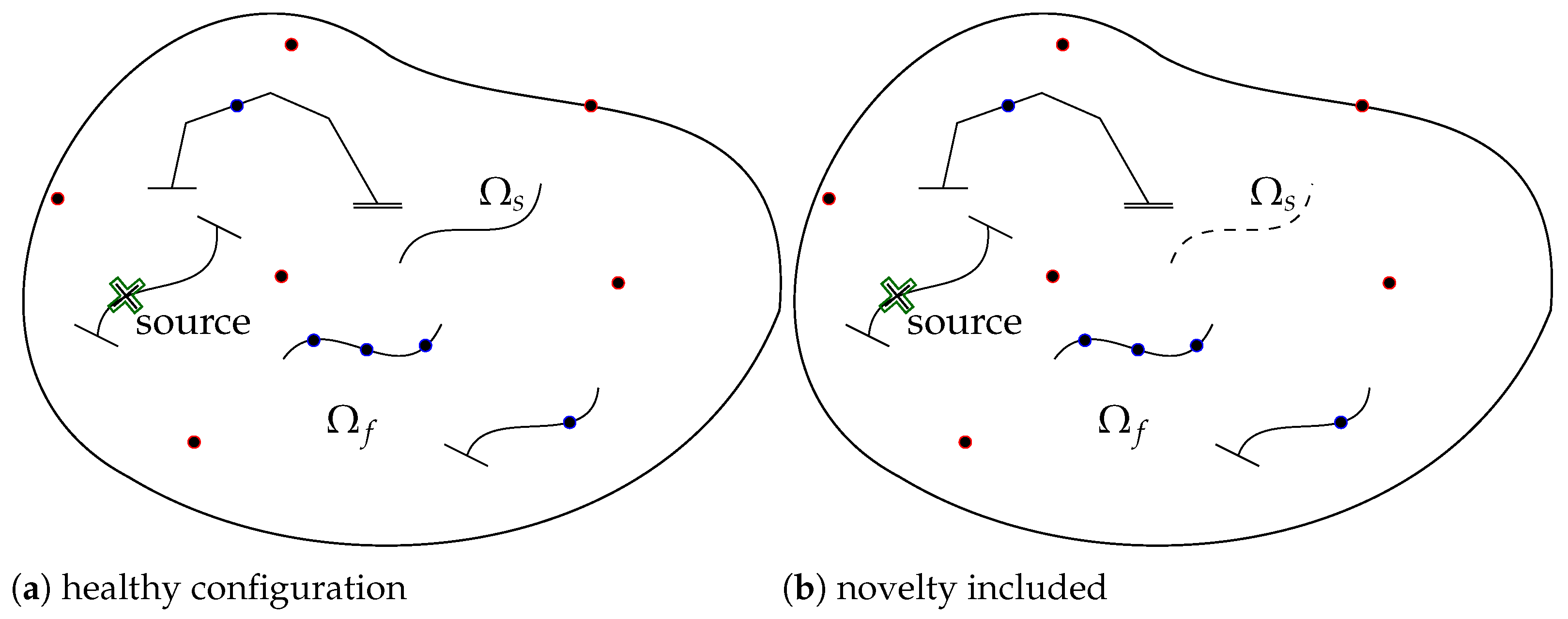
The second problem we are interested in is the localization of novelties taking place within the coupled vibro-acoustic system. These novelties may appear in either the acoustic or the mechanical elastic part. It is more common for such novelties to happen in the elastic part, e.g., in the form of some occurred damage on the elastic body or on the support of it. In order to find which part of the structural assembly has suffered such modifications and to accurately define its spatial location, we assume that such a novelty will act as a secondary source. Using the time reversibility of the waves, it is possible to localize this secondary source similarly to the original excitation source. In this case, to focus on the field produced by the novelty, we subtract the wavefield produced by the original source when the novelty did not exist. By using this latter signal, which is the difference of the fields recorded before and after the appearance of the novelty, we are able to localize the novelty.

Let us now describe the procedure to be numerically implemented using the descriptive sketch of Figure 1. For the source localization in a healthy medium, as shown in Figure 1a, a source acts as acoustic or mechanic excitation at time $t_0$, and the response to this excitation is recorded on a finite number of recording stations as pressure (via microphones) or kinematic responses (using accelerometers or displacement/velocity sensors) for a duration time T. We denote this wavefield $u_r$, including both acoustic and elastic responses, while the acquisition process is called the forward step. In the current computational approach, all data are obtained numerically using simulations of virtual experiments. Time reversibility assures us that reverting in time the recorded signals and re-emitting them as excitation, in a procedure called backward step, an energy focus will occur at the time $T-t_0$ on the spatial location of the original source. Note that actually, one needs to revert the whole wavefield and re-emit it, although it is well documented that the reduced (or incomplete) time reversal, where the signal is recorded at a finite number of sensors, still keeps the refocusing property. This is the source localization process, while for the novelty localization, a few extra datum are needed. In this case, we record the wavefield for a modified system configuration, which includes the novelty, e.g., some modification on one of the beams in the domain as depicted in Figure 1b; we call this wavefield $u_r^t$. By re-emitting the reversed signal of $u_r^t$, we expect to localize the original source by energy refocusing on its position at $T-t_0$, while for novelty, the localization will occur at time $T-t_0-t_1$, with $t_1$ being the time needed for the wave to travel from the source location to the novelty location. Finally, by re-emitting the signal resulting from the difference $u_r^n=u_r^t-u_r$, we expect again energy refocusing on the novelty position at time $T-t_0-t_1$.

3. Governing Equations of Structure and Acoustic Mediums and Their Coupling

We consider an elastic solid at equilibrium occupying the domain ${\Omega }_s$. The unknown displacement field of the solid is denoted by $u^s$, while linearized associated stress and strain tensors are indicated by $\epsilon \left(u^s\right)$ and $\sigma \left(u^s\right)$, respectively. The equation of motion for the solid, fixed on some part ${\Gamma }_u$ of the boundary and subject to a given force density $F^d$ on the rest boundary part ${\Gamma }_t$, is

$$\begin{array}{ccc}& \mathrm{div}\sigma \left(u^s\right)-{\varrho }_s\frac{{\partial }^2{u}^s}{\partial t^2}=f\hfill & \hfill \mathrm{in}{\Omega }_s,\end{array}$$

(1a)

$$\begin{array}{ccc}& u^s=0\hfill & \hfill \mathrm{on}{\Gamma }_u,\end{array}$$

(1b)

$$\begin{array}{ccc}& \sigma \left(u^s\right)n^s=F^d\hfill & \hfill \mathrm{on}{\Gamma }_t,\end{array}$$

(1c)

where here we have also assumed silent initial conditions. The acoustic domain is considered to be a compressible inviscid and irrotational fluid, where using the pressure scalar field p, the equation of motion is given as,

$$\begin{array}{ccc}& \frac{{\partial }^{2}p}{\partial t^2}-c_f^2{\nabla }^{2}p=c_f^2\frac{\partial q_f}{\partial t}\hfill & \hfill \mathrm{in}{\Omega }_f,\end{array}$$

(2a)

$$\begin{array}{ccc}& p=\tilde{p}\hfill & \hfill \mathrm{on}{\Gamma }_p,\end{array}$$

(2b)

$$\begin{array}{ccc}& \nabla p{n}^f=0\hfill & \hfill \mathrm{on}{\Gamma }_v,\end{array}$$

(2c)

$c_f$ being the speed of sound in the acoustic medium and $q_f$ the added mass per unit volume. Similar to the solid, the fluid is assumed to be at rest with silent initial conditions.

Now considering there is a part of the solid immersed or in touch with the fluid, we should appropriately consider the coupling of the domains and their responses. We denote that part as $\partial {\Omega }_c$, where the fluid particles and the solid move together in the normal direction of $\partial {\Omega }_c$. The normal unit vector external to the fluid is $n^f$ and on the common part $\partial {\Omega }_c$ is $n^f=-n^s$, with $n^s$ the normal unit vector external to the solid. We finally denote the unit normal as n, which is equal to $n^f$, while on $\partial {\Omega }_c$, the following holds,

$$\begin{array}{c}\hfill u^{s}n=u^{f}n\end{array}$$

(3)

together with the continuity of pressure,

$$\begin{array}{c}\hfill \sigma \left(u^s\right)n^s=-p.\end{array}$$

(4)

In order to couple the two different physics domains, a Neumann–Neumann approach [14] is followed, where Equation (4) is used for the realization of Equation (1c) and Equation (3) for Equation (2c), respectively. For the latter case, we use the linearized Euler equation, which because of Equation (3) takes the form,

$$\begin{array}{c}\hfill \nabla pn=-{\varrho }_f\frac{{\partial }^2{u}_s}{\partial t^2}n\end{array}$$

(5)

Without loss of generality, in this work we focus on structures consisting of beams or frame structures lying inside a two-dimensional acoustic field. Therefore, we consider here the case of a solid in the form of one-dimensional beam, as shown in Figure 2.

The above has been implemented using the SDE, which is a Java-based environment with numerical procedure capabilities [15]. This java numerical methods framework is mostly created by one of the authors. The implementation follows mainly the fluid–structure interaction approach, as implemented in CALFEM [16]. Verification has been further accomplished by comparing with results obtained from commercial finite element multiphysics software [17], with very good agreement. We should mention that in our implementation, we have adopted the assumption of pressure continuity on the beam’s line, which is a fair hypothesis for our problems, yet not appropriate to study problems of pressure gaps. Using finite elements for the vibro-acoustic system [18], the semi-discrete equation of motion [19] for the coupled system in matrix form, is

$$\left[\begin{array}{cc}{M}_s& 0\\ {\varrho }_f{c}_f^2{H}^T& M_f\end{array}\right]\left[\begin{array}{c}\ddot{d}\\ \ddot{p}\end{array}\right]+\left[\begin{array}{cc}{K}_s& -H\\ 0& K_f\end{array}\right]\left[\begin{array}{c}d\\ p\end{array}\right]=\left[\begin{array}{c}{f}_s\\ f_f\end{array}\right]$$

(6)

where $M_s$ and $K_s$ stands for the mass and stiffness matrices of the structural part and $M_f$ and $K_f$ for the fluid, respectively. The degrees of freedom indicated by d refer to kinematic variables (i.e., displacements and rotations) while p stands for the acoustic pressure and $f_s$, $f_f$ are excitation forces on the structural and acoustic part, respectively. Matrix H actually contains the coupling coefficients. Finally, some damping could be considered in the form of Rayleigh damping, among other possible models.

4. Computational Vibro-Acoustic Time Reversal

In computational time reversal, at least one of the two steps (forward or backward), is supposed to be performed numerically by using some appropriate method, e.g., finite differences or a finite element method (FEM), as it is conducted in this work. Here, we use the conventional FEM, which is very common for the solution of structural dynamics problems. We present numerical experiments both for data acquisition during the forward step as well as for refocusing during the backward step. The methodology could be described according to the set-up presented in Figure 1. Consider a coupled vibro-acoustic system, which is here represented by an acoustic field incorporating a number of beams and frame structures. In the forward step, we assume that a source (acoustic or mechanic) acts on some point $x_s$ and that the response $u_r\left(t\right)$ is recorded on some point $x_r$ for a time duration T. It is possible to record both acoustic pressure and kinematic motion signals. Then, in the backward step, the time reversed signal response $u_r(T-t)$ is re-emitted as excitation from the respective $x_r$ point. In that backward step, an energy refocusing will appear on the $x_s$ point after the same duration of time T. This main application is called source localization. Furthermore, another application is that of novelty localization, which considers location $x_d$ as the point at which a secondary source exists (novelty). In this case, we use the difference between the original signal and the one recorded after the novelty has been introduced. This can be expressed as:

$$\begin{array}{c}\hfill u_r^n=u_r^t-u_r\end{array}$$

(7)

In other words, $u_r^t$ contains both primal and secondary source influence on the response, $u_r$ contains only the influence of the original source, while $u_r^n$ the influence of the novelty related field. Therefore, by re-emitting (in the backward step) the signal reversed $u_r$ in time, one could locate the original source; by re-emitting $u_r^n$, one could locate the secondary source due to novelty; and finally, by $u_r^t$ re-emission, one could, possibly, locate both the original and secondary sources.

Of crucial importance is the choice of quantity to be monitored in order to observe the refocusing during the backward step. That is more prominent in the case of different physics domain coupling, where variables with different scales may coexist. The refocusing at an appropriate discrete time [5] or using time averaging techniques [20] will indicate the spatial location of the original source excitation used during the forward step. Regarding the monitoring quantity, here we consider the pressure field, while some more general quantity, e.g., the Euclidean norm of all the components of existing degrees of freedom on each spatial position, could also be appropriate.

For the source localization problem, we expect refocusing during the backward step, at the location of original source point at time $T-t_0$, $t_0$ being the peak of the pulse. The refocusing time in the novelty localization will be $T-t_0-t_1$, where $t_1$ is the time needed for the wave to propagate from the source point to the novelty location. Since the location of the novelty is the main unknown in our problem, the time $t_1$ is also unknown. A solution to this problem is to use a time average approach [20], or to utilize the evolution of appropriate measures (e.g., Shannon entropy, Bounded Variation) [21]. A simple yet efficient approach for defining the refocusing time could be based on the arrival time of waves from the source to the sensor while interacting with the novelty location [22]. More specifically, we can consider sensors (microphones) for the recording of the healthy configuration responses $u_r$ as well as $u_r^n$, as given in Equation (7). Using these signals, we can estimate the arrival time of $u_r^n$ as $t_r^{nov}$ and that of the original source’s incident wave $u_r$ as $t_r^{inc}$, while the difference of these time intervals,

$$\begin{array}{c}\hfill t_1^r=t_r^{nov}-t_r^{inc}\end{array}$$

(8)

is an estimation of time $t_1$ needed for the wave to travel from the source point to the novelty location. By using several sensors, we can derive an average time ${\tilde{t}}_1$, resulting hopefully in an improved estimate of the unknown time $t_1$. Then, the refocusing during the backward step should be expected to appear at time $T-t_0-{\tilde{t}}_1$.

5. Examples

We study two main examples in this section. The first one examines the source localization problem and the second one deals with the problem of novelty localization in the vibro-acoustic environment.

5.1. Source Localization Example

The rectangular domain with dimensions $H=0.1$ m and $L=H\sqrt{5}$, shown in Figure 3, is used in the forthcoming examples, which consists of three subdomains, while two structural elements in the form of the beams Beam 1 (horizontal) & Beam 2 (vertical) were introduced. The fluid’s density and sound speed are $\rho =1000$ kg/m${}^3$ and $c=1500$ m/s, respectively. The elastic material of the beams considered has Young’s modulus $E=68.9$ GPa, Poisson’s ratio $\nu =0.3$ and mass density $\varrho =2690{\mathrm{kg}/\mathrm{m}}^3$. Wave propagation was performed in time steps of $dt=1/F_s$ where $F_s=3\times 10$${}^6$ Hz. A minimum element size is prescribed in the finite element mesh such that the maximum distance traveled within an element in time step $dt$ to be $0.23$ of its representative length. The finite element mesh is comprised of 4213 quadrilateral elements with 368 on the boundary. There are 24 boundary receivers/emitters, 12 internal receivers/emitters, 5 receivers/emitters placed on the first structure (horizontal beam), and 7 receivers/emitters placed on the second structure (vertical beam), with 48 receivers/emitters in total.

The source used at the numerical simulations is a Ricker pulse

$$\begin{array}{c}\hfill f\left(t\right)=\left(1-2{\pi }^2{s}^2{(t-t_0)}^2\right)e^{-{\pi }^2{s}^2{(t-t_0)}^2}.\end{array}$$

(9)

with parameters $s=$ 37,740.14 s${}^{-1}$ and $t_0=3\times 10$ ${}^{-5}$ s. This pulse has, in the frequency domain, a median frequency of $40.759$ kHz, and a quite large bandwidth, spanning most of low frequencies before it falls gradually to $-60$ dB at 14 kHz. A plot of the pulse together with its spectrum is shown in Figure 4.

5.1.1. Comparison of SNRs with and without Structures

As mentioned above, we introduce structures in the domain (two beams in our case) and in this vibro-acoustic problem we are prompted to investigate whether the presence of the structures improves the SNR. By considering only the 24 boundary receivers/emitters, the recorded signals at the forward step were sent back, and for different simulation times, we calculated the SNRs for the two following cases. In the first case, there were not any structures in the domain, while in the second case, two beams (see Figure 3), were introduced. Shown in Figure 5 are the SNRs for both cases with their respective simulation duration. The longest duration of 84k time steps corresponds to a travel distance of $187L$, where L is the horizontal length of the domain. We notice that the presence of the beams improves the quality of focusing considerably, as expressed by the SNR values. This was an expected behaviour, since it has been observed that in random or general complex media the time reversal presents better refocusing properties [23].

It is worth mentioning that the presence of beams in the acoustic domain might be significant in the overall system’s response. In this context, we have tried to send back in the acoustic domain, during the backward time reversal step, the data recorded in the vibro-acoustic environment. As it was expected, the results were not acceptable. For example, in two experiments with simulation durations corresponding to $125L$ & $187L$ travel distances, at the expected source focusing times, the highest pressure values were not found at the source location. Considering this, we emphasize the importance of taking into account the presence of structural components into an acoustic domain and their interaction.

Remark 1.

This numerical example highlights the importance of the structural component. Indeed, we observe that when a structure is present, the complexity of the medium increases and this results in effectively improving the SNR. We also observe that the backward step does not focus on the source location when the structure is not taken into account. This last point raises some interesting questions regarding the accuracy with which the structure should be modeled. Further investigations in this direction will be the object of future work.

Remark 2.

We observe in Figure 5 that the SNR decreases as a function of time. One may think that this is due to the accumulated numerical phase error. However, although the error indeed accumulates as the time of the experiment increases, our numerical simulations suggest that this does not affect either the refocusing location or the SNR. In fact, it is well known that time-reversal focusing is very robust. Even one bit time reversal (i.e., when signals are digitized over one bit) has good focusing properties, as demonstrated in [24]. The decrease in SNR with time is attributed to the presence of ghosts, as explained in [3].

5.1.2. Using Signals Recorded on the Beams Only

Here, we present the results, in cases where signals recorded only on the beams were time reversed and emitted back to the domain from the emitters on the beams. The magnitudes of these signals are much smaller than those recorded at the boundaries (or inside the domain), so certain amplification would be necessary if we wish to combine the beam signals with those recorded in the fluid domain. In the last column of

Table 1. The SNR for some combinations of emitters on Beam 1 and Beam 2 and for total number of 28 k time steps.

Emitters on Beam 1	Emitters on Beam 2	SNR
1		1.08
1,2		1.12
1,5		1.64
	1	1.67
	1,7	1.55
1	1	1.83
5	7	2.83
3	4	2.29
1,5	1,7	2.28
1,2,3,4,5		1.88
	1,2,3,4,5,6,7	2.31
1,2,3,4,5	1,2,3,4,5,6,7	2.5

SNRs are reported for a simulation time of 28 k time steps (≈$62L$), and for several combinations of emitters on the beams. First, only one or two emitters are activated on each beam, then one from one beam and one from the other, then two and two, etc. Our observations regarding these experiments are the following: When there is only one emitter (on either beam) the SNR varies from 1.08 to 1.67. With two emitters on the same beam, the SNR lies between 1.55 and 1.64, while with one emitter on each beam the SNR increases and is between 1.83 and 2.29, and with two emitters on each beam the SNR is around 2.28, which is remarkable since when all emitters are active, the SNR value is 2.50. Moreover, since for another simulation duration of 8 k time steps, where we have either emitters 1 and 5 on beam 1 or emitters 1 and 7 on beam 2 we obtain SNRs, 1.61 and 1.51, respectively, we conclude that a large recording/emitting time is not necessarily needed in order to obtain a good SNR value.

When the domain is excited by all 12 (=5 + 7) emitters on the two beams, the SNR versus simulation duration is shown in Figure 6a. The maximum simulation duration of 28 ms corresponds to 84 k time steps or equivalently $187.7L$ distance traveled. We notice that the SNR stabilizes fairly quickly around the value of 2.49. A graph of the absolute pressure for a simulation duration of 9.333 ms corresponding to the last row of Table 1, is shown in Figure 6b.

Remark 3.

In this numerical example, we see that focusing on the source can be obtained even when recorders only on the structural component are available. The SNR in this case is lower than when receivers in the acoustic part are also used. The quality of the refocusing, as seen in Figure 6b, indicates that the source can be localized. The refocusing spot size depends on the pulse used. Since the width of the pulse is known, this information can be used to estimate the width of the peak. We should note, however, that this method does not allow for a precise estimation of the support of the source or the defect. It allows for the detection and localization by providing an estimate of where the source or the defect is located.

5.2. Novelty Localization Examples

The objective of this set of examples is to identify and localize novelties on certain components of a vibro-acoustic system. We formulate the problem by seeking which beam in the coupled structure acoustic system has undergone a modification with respect to its initial configuration. Generalizing, we may look for a vibro-acoustic system region that might have been subjected to some novelty. In order to succeed that, we utilize the time reversal property of the system using the difference response field given in Equation (7).

In all following numerical experiments, quantities that remain unchanged are the fluid density and sound speed ($\rho =1000$ kg/m${}^3$ and $c=1500$ m/s, respectively) and the numerical time integration step $dt=1/F_s$, where $F_s=3\times 10$${}^6$ Hz. The simulation durations of the experiments are declared in time steps $dt$ or equivalently in multiples of propagation domain lengths, L. The minimum element size in the finite element mesh is also kept constant, so that the maximum distance traveled during a time step $dt$ is $0.23$ of its representative length. The Ricker pulse center remains at time $t_0=3\times {10}^{-5}$ s, and its half time span (see Figure 4a) is approximately $\Delta t=2\times {10}^{-5}$ s.

5.2.1. Novelty Case A

Two experiments were run, experiment A1 and experiment A2. Meanwhile, at the healthy beam case, both beams had Pinned-Pinned (PP) boundary conditions (BC), in case A1 the horizontal beam’s right end is switched to a free BC, representing, for example, a support failure. The simulation time was 1.333 ms, which corresponds to 4000 time steps or a traveled distance, which is approximately $9L$, with L being the longest side of the rectangular domain. Since the center of the pulse is at time $t_0=3\times {10}^{-5}$ s and its half time span (see Figure 4a) is approximately $\Delta t=2\times {10}^{-5}$ s, considering the simulation time and the travel time to get to the novelty, the pulse midpoint should be found at the novelty at time $t_c=1.291$ ms, while the activity at the novelty should present itself between times: $t_c-\Delta t=1.271$ ms and $t_c+\Delta t=1.311$ ms.

Shown in Figure 7 is the pressure time history at the point of the novelty, in which several peaks are identified at last part of the simulation. They represent pressure activity at the novelty location. To be mentioned that time reversed signals have been re-emitted back form the 24 stations located onto the boundary.

A characteristic shot of the entire domain’s absolute pressure at time step 3624, which corresponds to $1.208$ ms, is given in Figure 8. The defect is clearly revealed at the right end of the horizontal (see also Figure 3), which has undergone the support modification.

In case A2, the change of the vertical beam’s top end boundary condition to a free end was considered as the novelty. The simulation time was again 1.333 ms, which corresponds to 4000 time steps or a $9L$ traveled distance. The calculated travel time for the Ricker’s pulse midpoint to reach the novelty is $t_t=42.325$ ms. The center of the pulse should reach the novelty at time $t_c=1.274$ ms, while the activity at the novelty should present itself between times: $t_c-\Delta t=1.254$ ms and $t_c+\Delta t=1.294$ ms. By looking at the pressure time series at the novelty (see Figure 9), we observe once again that several peaks are identified.

A characteristic plot of the absolute pressure on the whole domain at time $1.212$ ms, corresponding to the highest pressure peak (time step 3638), is shown in Figure 10, where it is evident that the pressure activity is located exactly at the top end of the vertical beam, where the novelty lies.

5.2.2. Novelty Case B

In this case, two experiments, B1 & B2, were also run. In experiment B1, the second segment from the left of the horizontal beam (segments defined between the distinct emitters, as shown in Figure 3), had a Young modulus 10 times smaller compared to the healthy beam value, simulating thus a damaged beam, while at experiment B2, the third segment from the bottom of the vertical beam had a Young modulus 10 times smaller. In both cases, the beams had Pinned-Pinned boundary conditions and emitters 1–24 were activated. The pressure time history at the point of the novelty on the horizontal beam is shown in Figure 11. The absolute pressure of the entire domain at the time instance of the global absolute pressure extreme, step 3559 (=1.186 ms), is depicted in Figure 12. We observe a dipole-like source focusing at the place of the damaged beam. This kind of activity is not observed if we look at the location of the healthy horizontal beam at any time instance.

When the novelty is defined as a defective segment (the 3rd segment from the bottom) of the vertical beam, the pressure time history for a simulation duration of 4 k steps at the midpoint of this segment, is shown in Figure 13. The absolute pressure of the entire domain at time step 3691 (time instance = 1.230 ms), is depicted in Figure 14. Again, pressure activity is evident at the vicinity of the damaged beam segment.

5.2.3. Novelty Case C

In this example, we are trying to see whether it is possible to detect novelties at a structure by exciting the medium with forces resulting from the recorded structural kinematic responses (accelerations, velocities or displacements) on another one. Thus, in this section, we are actually examining the possibility of detecting a novelty at one beam by emitting signals recorded at the other beam. All five emitters of the horizontal beam, which had been recording displacements, are the only ones made active, while the defect to be detected is at the top end boundary condition of the vertical beam, which is made free in the backward step of the experiment.

The pressure time history for a simulation duration of 4k steps at the top point of the vertical beam, is shown in Figure 15. The absolute pressure of the entire domain at time step 3632 (time instance = 1.210 ms), is depicted in Figure 16. Again, pressure activity is evident at the top end of the vertical beam. We should mention that if the kinematic signals recorded at the beams (or at any other structure), are going to be used solely, or in combination with other emitters in the domain, for an ample excitation of the medium at the backward stage, an adequate level of signal amplification should definitely be considered. The amount of amplification should depend on the radiation efficiency of the structure under consideration.

Remark 4.

Our numerical results illustrate that the proposed methodology allows for novelty detection and localization. Receivers may be placed in the acoustic part and/or the structural component. Qualitatively different refocusing is observed for different types of defects. Two defect types were considered here a support failure modeled by modifying the BC at the end of a beam and a beam that is damaged in the interior modeled by modifying the Young modulus. Future work may exploit these different qualitative focusing properties to distinguish between different types of defects.

6. Conclusions

In this work, we have numerically studied the applicability of a time reversal for source and novelty detection and localization in a vibro-acoustic environment. The necessary computational setup regarding the coupling between the acoustic fluid and the structural components, which are here represented by beams, along with all the adopted simplifications and approximations, has been presented. The implemented numerical framework was used for two problems. The first one deals with the localization of some source that originally excites the vibro-acoustic system and the second with the problem of localizing some novelties presented at some components of the system. It has been demonstrated that both problems can be successfully addressed. It was also demonstrated that accounting for the presence of structural components and their coupling within the acoustic domain is important and improves the results, leading to higher SNR values. The advantage of the presented methodology is that it is rather simple and therefore easy to use in practical applications. A possible disadvantage is the accuracy with which the structure should be modeled. Further investigations in this direction, considering the complex environments of fully three dimensional elastodynamic domains coupled with acoustic fluids, would be a natural extension of this work.

References

1. Fink, M.; Prada, C. Acoustic time-reversal mirrors. Inverse Probl. 2001, 17, R1. [Google Scholar] [CrossRef] [Green Version]
2. Givoli, D. Time reversal as a computational tool in acoustics and elastodynamics. J. Comput. Acoust. 2014, 22, 1430001. [Google Scholar] [CrossRef]
3. Petromichelakis, I.; Tsogka, C.; Panagiotopoulos, C. Signal-to-Noise Ratio analysis for time-reversal based imaging techniques in bounded domains. Wave Motion 2018, 79, 23–43. [Google Scholar] [CrossRef]
4. Panagiotopoulos, C.G.; Petromichelakis, Y.; Tsogka, C. Time reversal in elastodynamics with application to structural health monitoring. In Proceedings of the 5th International Conference on Computational Methods in Structural Dynamics and Earthquake Engineering, Crete Island, Greece, 25–27 May 2015. [Google Scholar]
5. Panagiotopoulos, C.; Petromichelakis, Y.; Tsogka, C. Time reversal and imaging for structures. In Dynamic Response of Infrastructure to Environmentally Induced Loads; Springer: Abingdon, UK, 2017; pp. 159–182. Available online: https://link.springer.com/book/10.1007/978-3-319-56136-3#about-this-book (accessed on 28 September 2022).
6. Panagiotopoulos, C.G.; Stavroulakis, G.E. A Numerical Study on Computational Time Reversal for Structural Health Monitoring. Signals 2021, 2, 225–244. [Google Scholar] [CrossRef]
7. Draeger, C.; Cassereau, D.; Fink, M. Acoustic time reversal with mode conversion at a solid-fluid interface. Appl. Phys. Lett. 1998, 72, 1567–1569. [Google Scholar] [CrossRef]
8. Tsogka, C.; Papanicolaou, G.C. Time reversal through a solid–liquid interface and super-resolution. Inverse Probl. 2002, 18, 1639. [Google Scholar] [CrossRef]
9. van Ophem, S.; Deckers, E.; Atak, O.; Desmet, W. Vibro-acoustic fault detection using a numerical time reversal method with reduced order models. In Proceedings of the 8th European Workshop on Structural Health Monitoring, Bilbao, Spain, 5–8 July 2016. [Google Scholar]
10. Amitt, E.; Givoli, D.; Turkel, E. Time reversal for crack identification. Comput. Mech. 2014, 54, 443–459. [Google Scholar] [CrossRef]
11. Becht, P.; Deckers, E.; Claeys, C.; Pluymers, B.; Desmet, W. Loose bolt detection in a complex assembly using a vibro-acoustic sensor array. Mech. Syst. Signal Process. 2019, 130, 433–451. [Google Scholar] [CrossRef]
12. Becht, P.; Deckers, E.; Claeys, C.; Pluymers, B.; Desmet, W. Selection of Small Sensor Arrays for Localization of Damage in Complex Assemblies Using Vibro-Acoustic Signals. In Proceedings of the 13th International Conference on Damage Assessment of Structures, Porto, Portugal, 9–10 July 2019; Springer: Singapore, 2020; pp. 263–282. [Google Scholar]
13. Lopatin, C.; Rabinovich, D.; Givoli, D.; Turkel, E. Computational time reversal for NDT applications using experimental data. J. Nondestruct. Eval. 2017, 36, 48. [Google Scholar] [CrossRef]
14. Quarteroni, A.; Valli, A. Domain Decomposition Methods for Partial Differential Equations; Oxford University Press: Oxford, UK, 1999. [Google Scholar]
15. Panagiotopoulos, C. Symplegma Project. Available online: http://symplegma.org/ (accessed on 28 September 2022).
16. Dahlblom, O.; Peterson, A.; Petersson, H. CALFEM—A program for computer-aided learning of the finite element method. Eng. Comput. 1986, 3, 155–160. [Google Scholar] [CrossRef]
17. COMSOL AB. COMSOL Multiphysics®v. 4.4. Available online: www.comsol.com (accessed on 28 September 2022).
18. Sandberg, G.; Ohayon, R. Computational Aspects of Structural Acoustics and Vibration; Springer Science & Business Media: Berlin, Germany, 2009; Volume 505. [Google Scholar]
19. Belytschko, T.; Hughes, T.J. Computational methods for transient analysis. Amst. N.-Holl. (Comput. Methods Mech.) 1983, 1. [Google Scholar] [CrossRef] [Green Version]
20. Koo, S.; Karve, P.M.; Kallivokas, L.F. A comparison of time-reversal and inverse-source methods for the optimal delivery of wave energy to subsurface targets. Wave Motion 2016, 67, 121–140. [Google Scholar] [CrossRef]
21. Derveaux, G.; Papanicolaou, G.; Tsogka, C. Time reversal imaging for sensor networks with optimal compensation in time. J. Acoust. Soc. Am. 2007, 121, 2071–2085. [Google Scholar] [CrossRef] [PubMed] [Green Version]
22. Amitt, E.; Givoli, D.; Turkel, E. Combined arrival-time imaging and time reversal for scatterer identification. Comput. Methods Appl. Mech. Eng. 2017, 313, 279–302. [Google Scholar] [CrossRef]
23. Borcea, L.; Papanicolaou, G.; Tsogka, C. Time and direction of arrival detection and filtering for imaging in strongly scattering random media. Waves Random Complex Media 2017, 27, 664–689. [Google Scholar] [CrossRef] [Green Version]
24. Derode, A.; Tourin, A.; Fink, M. Ultrasonic pulse compression with one-bit time reversal through multiple scattering. J. Appl. Phys. 1999, 85, 6343–6352. [Google Scholar] [CrossRef]
Figure 1. A schematic representation of the computational time reversal experimental set-up. On the left, a schematic of the healthy configuration is shown. On the right the same configuration is presented, including the novelty on the structure indicated with the dashed-line beam. Red and blue dots are assumed to be pressure and kinematic response recorders, respectively.
Signals 03 00043 g001
Figure 2. Beam fully immersed in the fluid. The beam element has been implemented as two node straight line element. On the beam’s axis, it is assumed that there is continuity of pressure.
Signals 03 00043 g002
Figure 3. The domain with two beams immersed in the fluid and 48 receivers/emitters in total.
Signals 03 00043 g003
Figure 4. The Ricker pulse used in the numerical experiments and its spectrum.
Signals 03 00043 g004
Figure 5. SNRs vs simulation time for when beams are and are not present inside the domain.
Signals 03 00043 g005
Figure 6. The SNR vs simulation duration when all emitters on the beams are active (corresponding to the last row of Table 1).
Signals 03 00043 g006
Figure 7. Backward step pressure time history, at the point of the novelty on the horizontal beam.
Signals 03 00043 g007
Figure 8. Absolute pressure on the whole domain at time 1.208 ms. Beams are plotted with light blue color. The defect is clearly revealed at the right end of the horizontal beam.
Signals 03 00043 g008
Figure 9. Pressure time history at the point of the novelty of the vertical beam.
Signals 03 00043 g009
Figure 10. The absolute pressure on the whole domain at time 1.212 ms. Beams are plotted with light blue color. Pressure activity is evident at the top of the vertical beam.
Signals 03 00043 g010
Figure 11. Pressure time history at the middle point of the 2nd segment of the horizontal beam. This segment’s Young modulus is 10 times smaller compared to the values of the remaining segments.
Signals 03 00043 g011
Figure 12. The absolute pressure on the whole domain at time 1.186 ms. Beams are plotted with light blue color and the location of the defect is indicated with yellow color. Dipole-like pressure activity is evident at the vicinity of the damaged segment of the beam.
Signals 03 00043 g012
Figure 13. Pressure time history at the midpoint of the 3rd segment of the vertical beam. This segment’s Young modulus is 10 times smaller compared to the values of the remaining segments.
Signals 03 00043 g013
Figure 14. The absolute pressure on the whole domain at time 1.230 ms. Beams are plotted with light blue color and the location of the defect is indicated with yellow color. Pressure activity is evident at the vicinity of the damaged segment of the beam.
Signals 03 00043 g014
Figure 15. Pressure time history at the top end of the vertical beam.
Signals 03 00043 g015
Figure 16. The absolute pressure on the whole domain at time 1.210 ms. Beams are plotted with light blue color. Pressure activity is evident at the top end of the vertical beam.
Signals 03 00043 g016