
Continuous Adaptation with Online Meta-Learning for Non-Stationary Target Regression Tasks


Abstract
:1. Introduction
- We propose a method to adapt to a non-stationary target (concept drift) consisting of two components: Offline/Online Bayesian meta-learning (empirical Bayes) and Bayesian regression with sliding window.
- We show that these components work complementarily and achieve good performance for both stationary and non-stationary tasks.
- We decompose the algorithm with a computationally efficient recursive form.
2. Preliminaries
2.1. Bayesian Linear Regression
2.2. Offline Meta-Learning
3. The CORAL Algorithm
3.1. Non-Stationary Target Adaptation
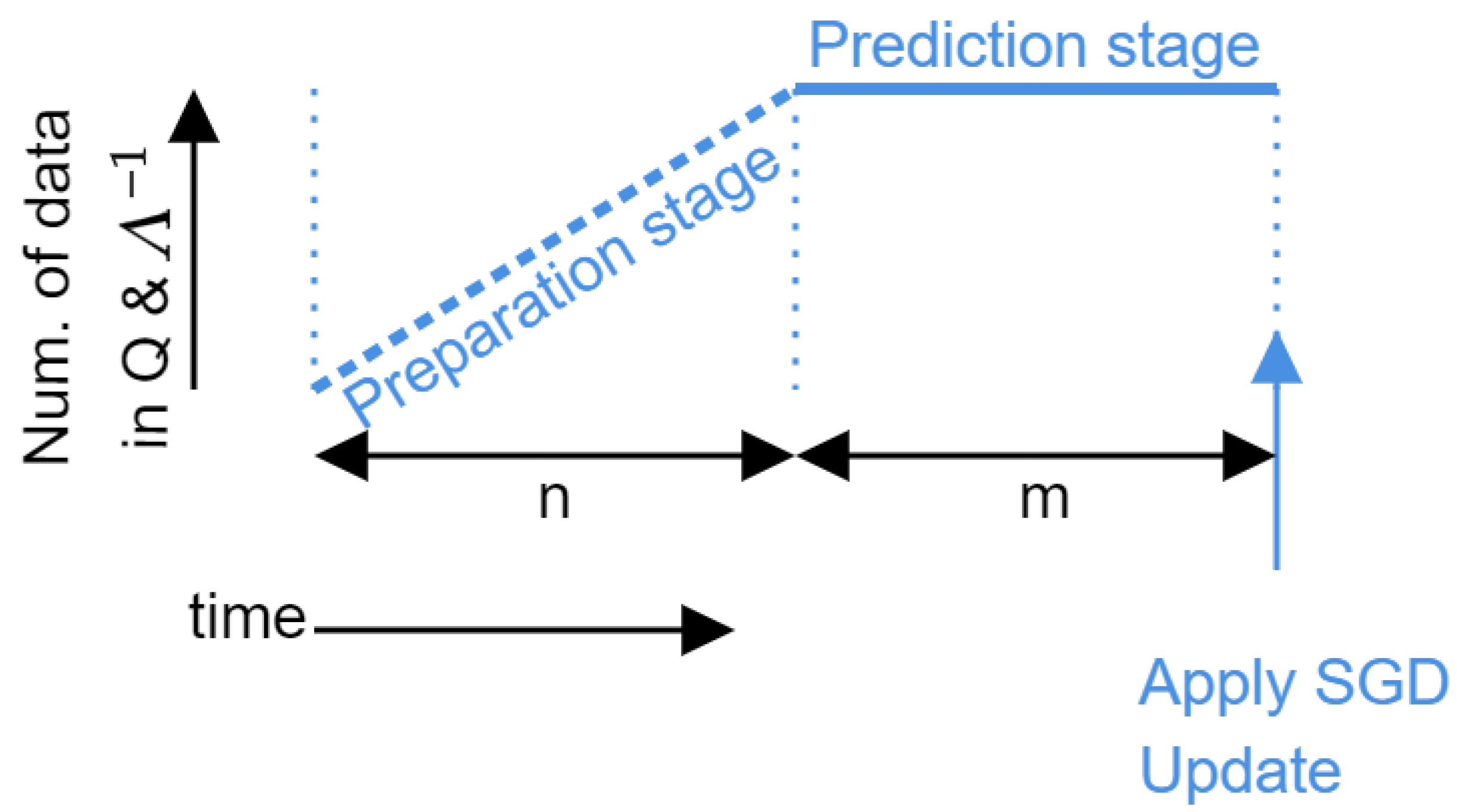
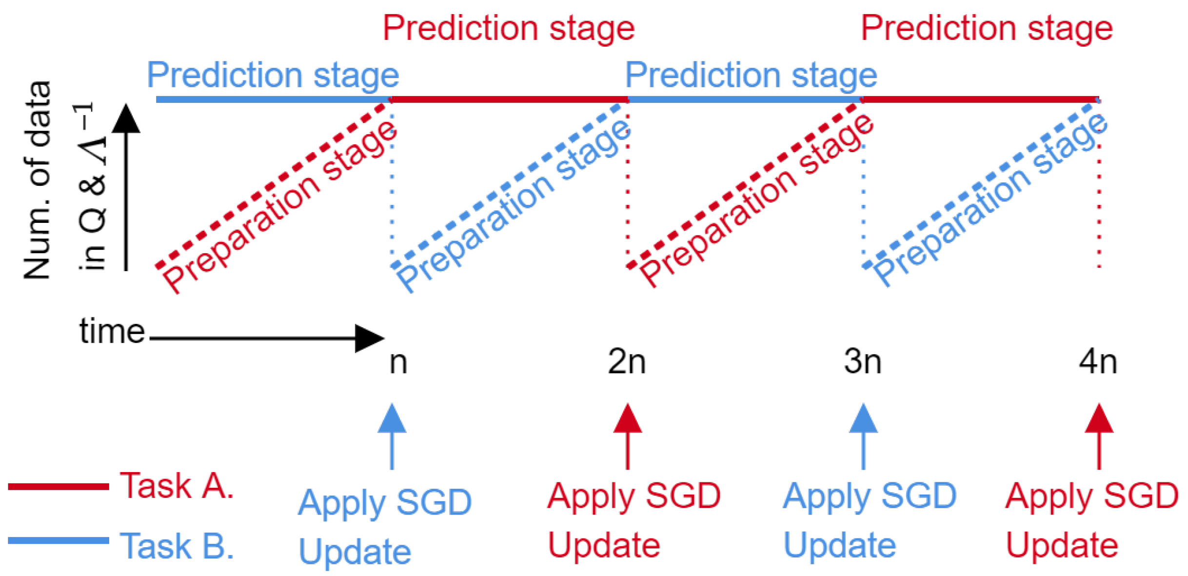
3.2. Online Meta-Learning
| Algorithm 1 One cycle of the CORAL algorithm. |
Require: and
|
4. Related Work
4.1. Sliding Windows
4.2. Forgetting Methods
4.3. Kalman Filter
5. Evaluation
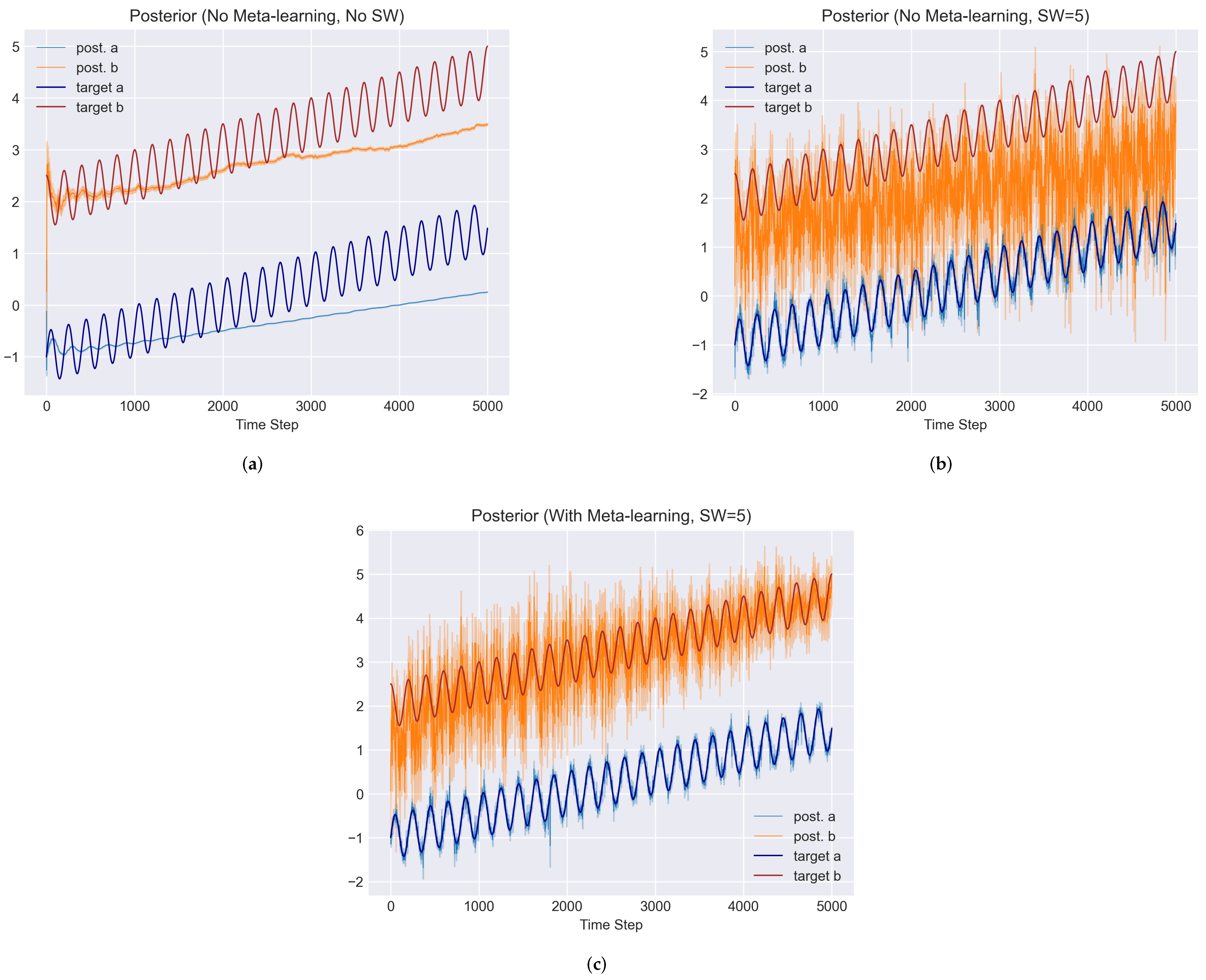
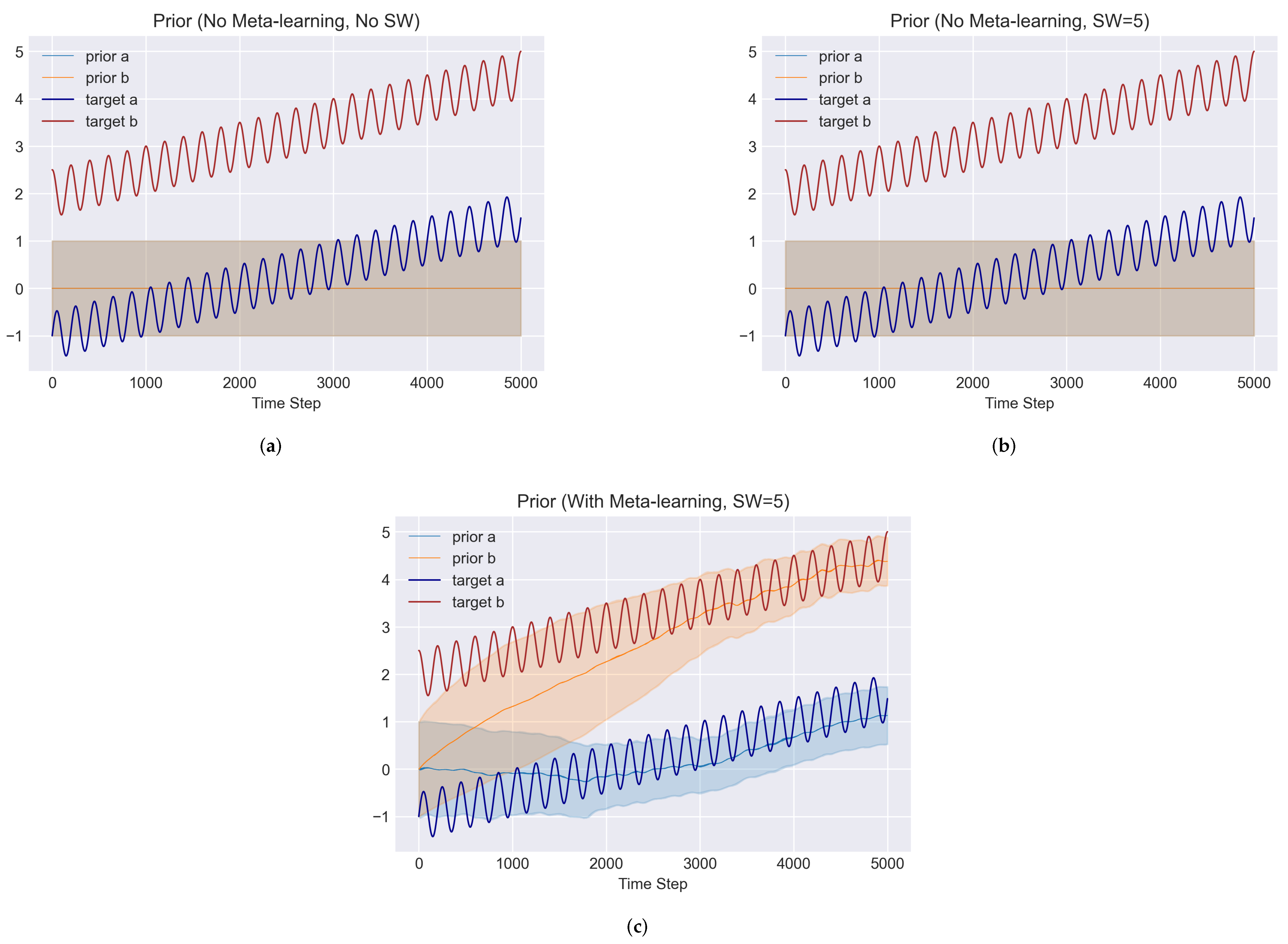
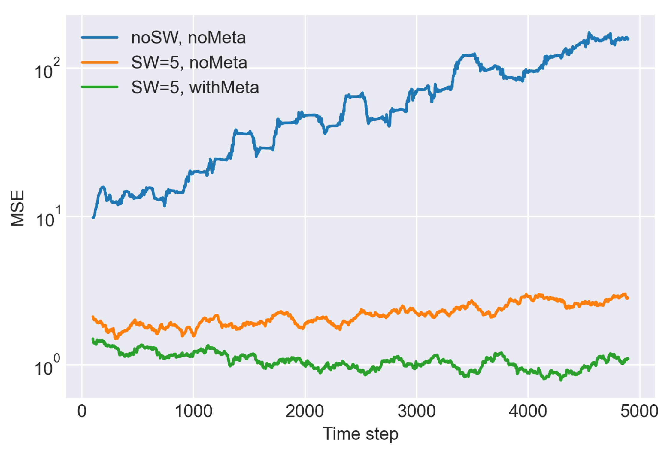
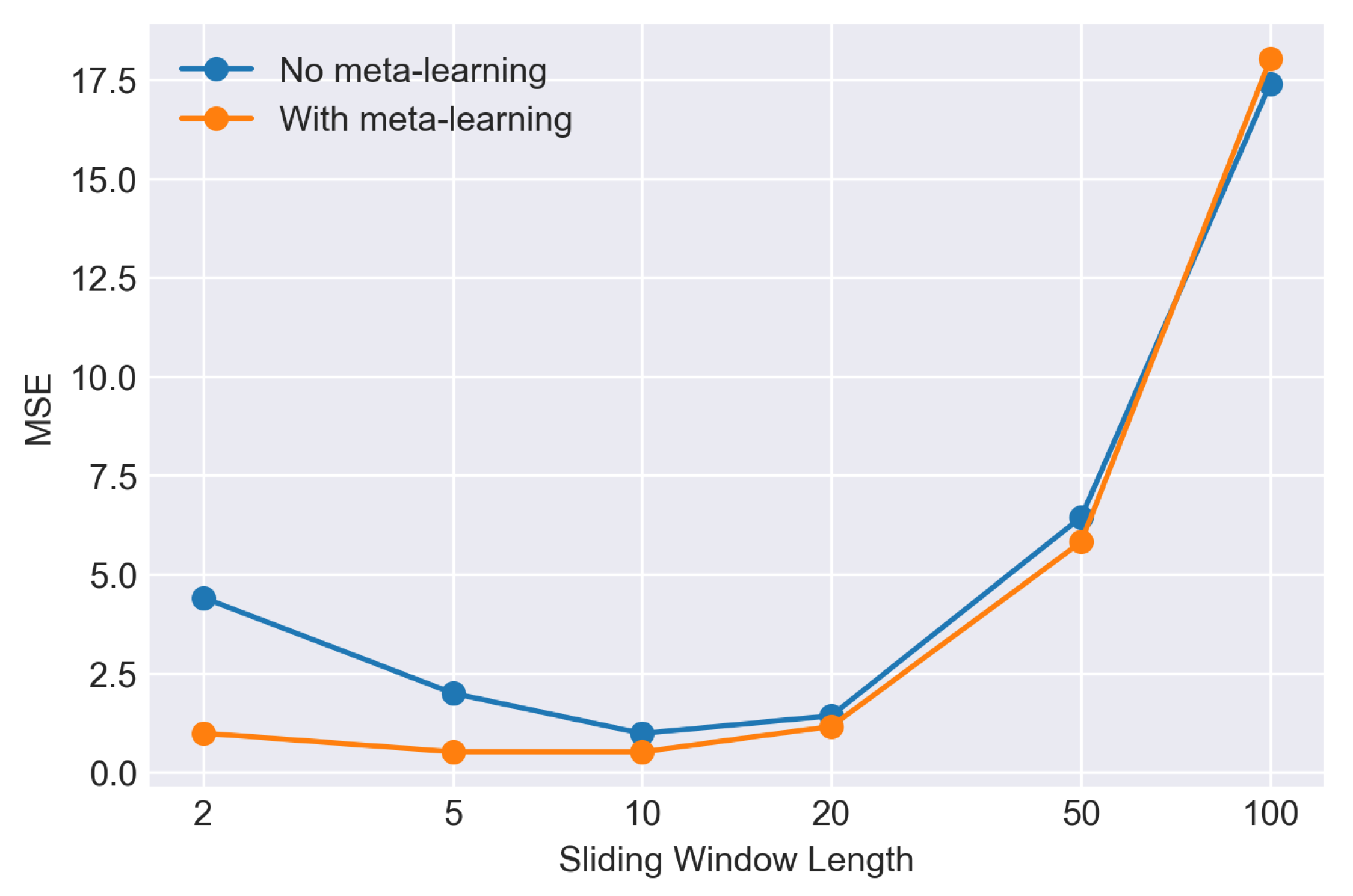
5.1. Toy Problem
5.2. Blood Glucose Level Prediction
5.2.1. Data Generation
5.2.2. Predictor Model
5.2.3. Evaluation Procedure
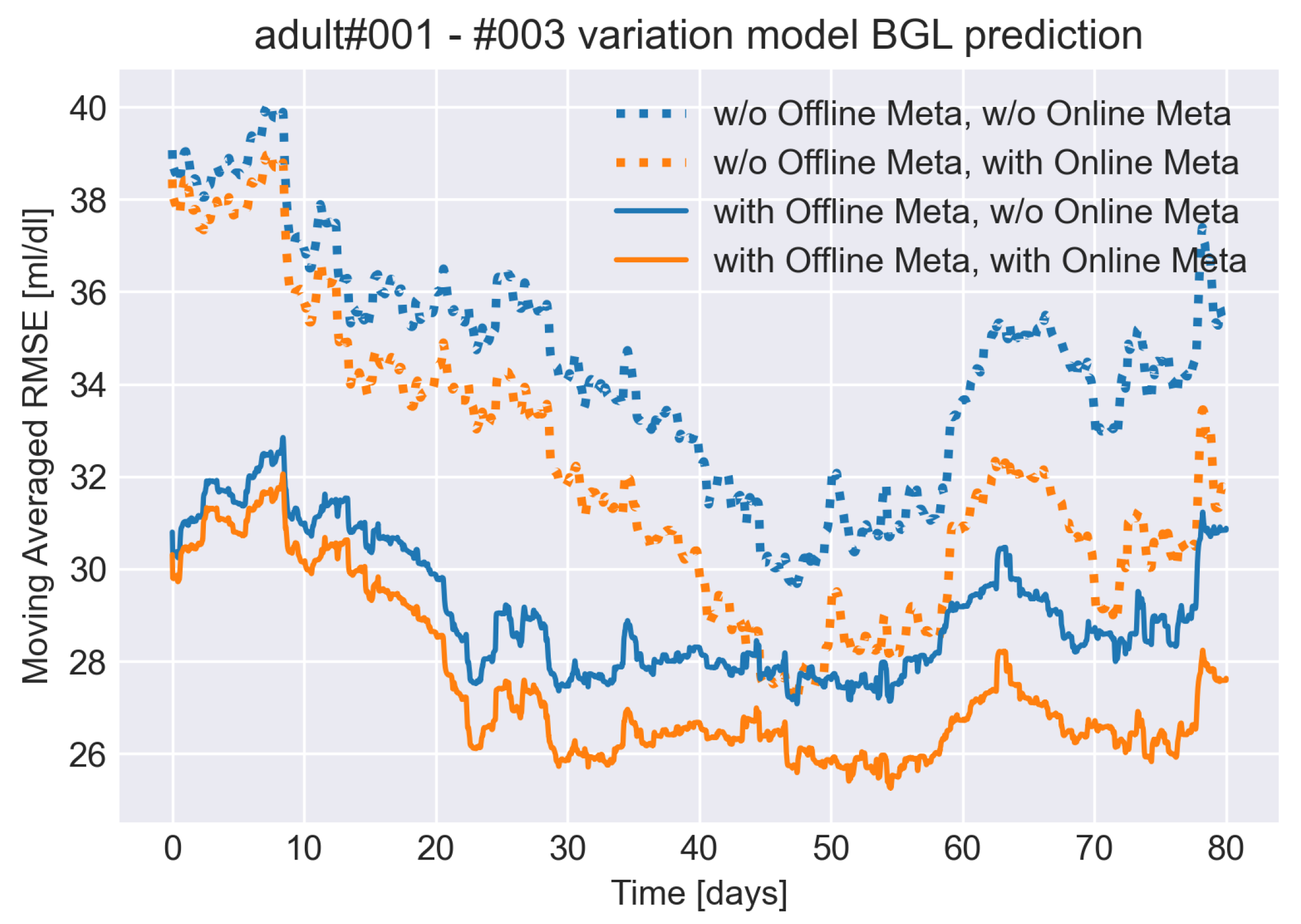
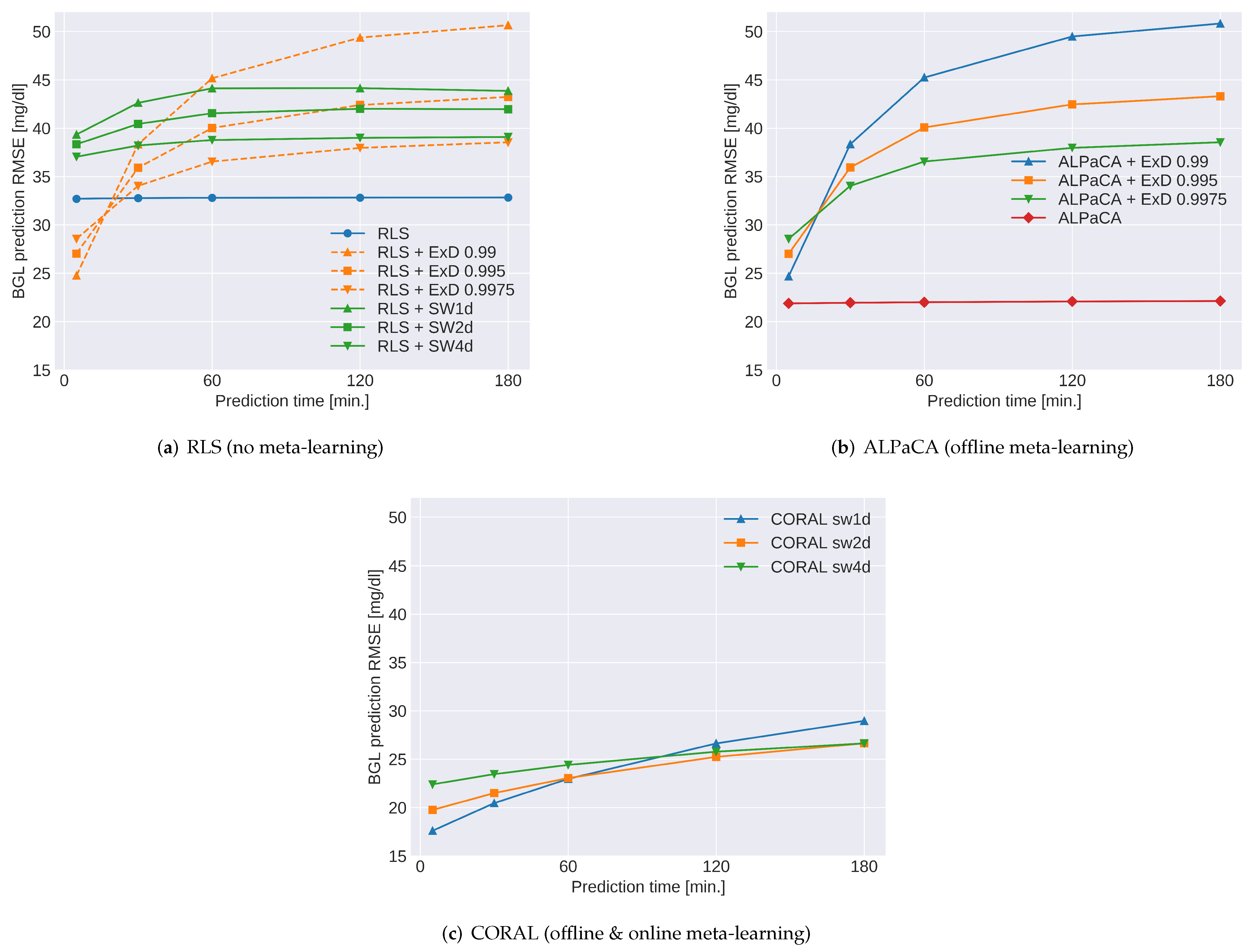
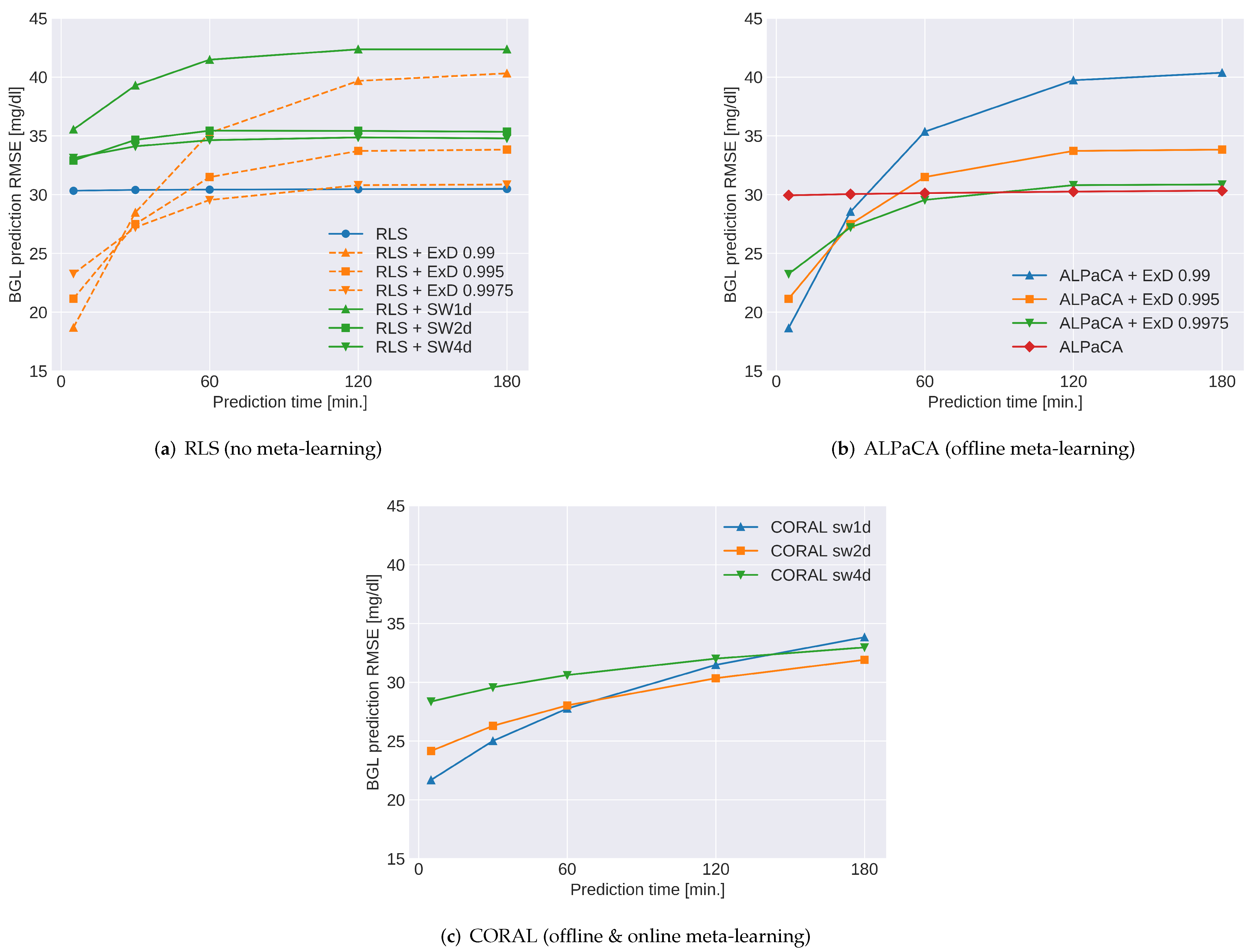
5.2.4. Results
6. Conclusions
Author Contributions
Funding
Institutional Review Board Statement
Informed Consent Statement
Data Availability Statement
Acknowledgments
Conflicts of Interest
References
- Gama, J.; Žliobaite, I.; Bifet, A.; Pechenizkiy, M.; Bouchachia, A. A survey on concept drift adaptation. ACM Comput. Surv. (CSUR) 2014, 46, 1–37. [Google Scholar] [CrossRef]
- Carmona-Cejudo, J.M.; Baena-Garcia, M.; del Campo-Avila, J.; Morales-Bueno, R.; Bifet, A. Gnusmail: Open Framework for On-Line Email Classification; IOS Press: Amsterdam, The Netherlands, 2011. [Google Scholar]
- Bifet, A.; Frank, E. Sentiment knowledge discovery in twitter streaming data. In Proceedings of the International Conference on Discovery Science, Thessaloniki, Greece, 19–21 October 2010; pp. 1–15. [Google Scholar]
- Al-Shedivat, M.; Bansal, T.; Burda, Y.; Sutskever, I.; Mordatch, I.; Abbeel, P. Continuous adaptation via meta-learning in nonstationary and competitive environments. arXiv 2017, arXiv:1710.03641. [Google Scholar]
- Amit, R.; Meir, R. Meta-learning by adjusting priors based on extended PAC-Bayes theory. In Proceedings of the International Conference on Machine Learning, Stockholm, Sweden, 10–15 July 2018; pp. 205–214. [Google Scholar]
- Ravi, S.; Beatson, A. Amortized Bayesian Meta-Learning. In Proceedings of the ICLR (Poster), New Orleans, LA, USA, 6–9 May 2019. [Google Scholar]
- Grant, E.; Finn, C.; Levine, S.; Darrell, T.; Griffiths, T. Recasting gradient-based meta-learning as hierarchical bayes. arXiv 2018, arXiv:1801.08930. [Google Scholar]
- Morris, C.N. Parametric empirical Bayes inference: Theory and applications. J. Am. Stat. Assoc. 1983, 78, 47–55. [Google Scholar] [CrossRef]
- Bauer, M.; Rojas-Carulla, M.; Świkatkowski, J.B.; Schölkopf, B.; Turner, R.E. Discriminative k-shot learning using probabilistic models. arXiv 2017, arXiv:1706.00326. [Google Scholar]
- Patacchiola, M.; Turner, J.; Crowley, E.J.; O’Boyle, M.; Storkey, A. Bayesian Meta-Learning for the Few-Shot Setting via Deep Kernels. In Proceedings of the 34th International Conference on Neural Information Processing Systems, Montreal, QC, Canada, 6–12 December 2020. [Google Scholar]
- Moreno-Torres, J.G.; Raeder, T.; Alaiz-Rodríguez, R.; Chawla, N.V.; Herrera, F. A unifying view on dataset shift in classification. Pattern Recognit. 2012, 45, 521–530. [Google Scholar] [CrossRef]
- Kull, M.; Flach, P. Patterns of dataset shift. In Proceedings of the First International Workshop on Learning over Multiple Contexts (LMCE) at ECML-PKDD, Nancy, France, 15–19 September 2014. [Google Scholar]
- Harrison, J.; Sharma, A.; Pavone, M. Meta-learning priors for efficient online bayesian regression. In International Workshop on the Algorithmic Foundations of Robotics; Springer: Berlin/Heidelberg, Germany, 2018; pp. 318–337. [Google Scholar]
- Golub, G.H.; Van Loan, C.F. Matrix Computations; JHU Press: Baltimore, MD, USA, 2013; Volume 3. [Google Scholar]
- Finn, C.; Abbeel, P.; Levine, S. Model-agnostic meta-learning for fast adaptation of deep networks. In Proceedings of the 34th International Conference on Machine Learning—ICML 2017, Sydney, Australia, 6–11 August 2017; Volume 3, pp. 1856–1868. [Google Scholar]
- Yoon, J.; Kim, T.; Dia, O.; Kim, S.; Bengio, Y.; Ahn, S. Bayesian model-agnostic meta-learning. In Proceedings of the 32nd International Conference on Neural Information Processing Systems, Montréal, QC, Canada, 3–8 December 2018; pp. 7343–7353. [Google Scholar]
- Finn, C.; Xu, K.; Levine, S. Probabilistic model-agnostic meta-learning. arXiv 2018, arXiv:1806.02817. [Google Scholar]
- Sayed, A.H. Adaptive Filters; John Wiley & Sons: Hoboken, NJ, USA, 2011. [Google Scholar]
- Harrison, J.; Sharma, A.; Finn, C.; Pavone, M. Continuous meta-learning without tasks. arXiv 2019, arXiv:1912.08866. [Google Scholar]
- Adams, R.P.; MacKay, D.J.C. Bayesian online changepoint detection. arXiv 2007, arXiv:0710.3742. [Google Scholar]
- Haykin, S.S. Introduction to Adaptive Filters; Macmillan: London, UK, 1984. [Google Scholar]
- Kulhavỳ, R.; Kárnỳ, M. Tracking of slowly varying parameters by directional forgetting. IFAC Proc. Vol. 1984, 17, 687–692. [Google Scholar] [CrossRef]
- Parkum, J.E.; Poulsen, N.K.; Holst, J. Recursive forgetting algorithms. Int. J. Control 1992, 55, 109–128. [Google Scholar] [CrossRef]
- Kalman, R.E. A New Approach to Linear Filtering and Prediction Problems; The American Society of Mechanical Engineers: New York, NY, USA, 1960. [Google Scholar]
- Stepanov, O. Kalman filtering: Past and present. An outlook from Russia. (On the occasion of the 80th birthday of Rudolf Emil Kalman). Gyroscopy Navig. 2011, 2, 99–110. [Google Scholar] [CrossRef]
- Huang, Y.; Zhang, Y.; Wu, Z.; Li, N.; Chambers, J. A novel adaptive Kalman filter with inaccurate process and measurement noise covariance matrices. IEEE Trans. Autom. Control 2017, 63, 594–601. [Google Scholar] [CrossRef] [Green Version]
- Mohamed, A.; Schwarz, K. Adaptive Kalman filtering for INS/GPS. J. Geod. 1999, 73, 193–203. [Google Scholar] [CrossRef]
- Sage, A.P.; Husa, G.W. Adaptive filtering with unknown prior statistics. Jt. Autom. Control Conf. 1969, 7, 760–769. [Google Scholar]
- Gao, X.; You, D.; Katayama, S. Seam tracking monitoring based on adaptive Kalman filter embedded Elman neural network during high-power fiber laser welding. IEEE Trans. Ind. Electron. 2012, 59, 4315–4325. [Google Scholar] [CrossRef]
- Sarkka, S.; Nummenmaa, A. Recursive noise adaptive Kalman filtering by variational Bayesian approximations. IEEE Trans. Autom. Control 2009, 54, 596–600. [Google Scholar] [CrossRef]
- Ardeshiri, T.; Özkan, E.; Orguner, U.; Gustafsson, F. Approximate Bayesian smoothing with unknown process and measurement noise covariances. IEEE Signal Process. Lett. 2015, 22, 2450–2454. [Google Scholar] [CrossRef] [Green Version]
- Alberti, K.G.M.M.; Zimmet, P.Z. Definition, diagnosis and classification of diabetes mellitus and its complications. Part 1: Diagnosis and classification of diabetes mellitus. Provisional report of a WHO consultation. Diabet. Med. 1998, 15, 539–553. [Google Scholar] [CrossRef]
- Davis, A.K.; DuBose, S.N.; Haller, M.J.; Miller, K.M.; DiMeglio, L.A.; Bethin, K.E.; Goland, R.S.; Greenberg, E.M.; Liljenquist, D.R.; Ahmann, A.J.; et al. Prevalence of detectable C-peptide according to age at diagnosis and duration of type 1 diabetes. Diabetes Care 2015, 38, 476–481. [Google Scholar] [CrossRef] [PubMed] [Green Version]
- Dalla Man, C.; Micheletto, F.; Lv, D.; Breton, M.; Kovatchev, B.; Cobelli, C. The UVA/PADOVA type 1 diabetes simulator: New features. J. Diabetes Sci. Technol. 2014, 8, 26–34. [Google Scholar] [CrossRef] [Green Version]
- Xie, J. Simglucose v0.2.1. 2018. Available online: https://github.com/jxx123/simglucose (accessed on 28 December 2019).
- Mikines, K.J.; Sonne, B.; Farrell, P.A.; Tronier, B.; Galbo, H. Effect of physical exercise on sensitivity and responsiveness to insulin in humans. Am. J. Physiol. Endocrinol. Metab. 1988, 254, E248–E259. [Google Scholar] [CrossRef] [PubMed]
- Mikines, K.J.; Sonne, B.; Tronier, B.; Galbo, H. Effects of acute exercise and detraining on insulin action in trained men. J. Appl. Physiol. 1989, 66, 704–711. [Google Scholar] [CrossRef]
- Gürbilek, N. Real-Time Computing without Stable States: A New Framework for Neural Computation Based on Perturbations. J. Chem. Inf. Model. 2013, 53, 1689–1699. [Google Scholar] [CrossRef]
- Jaeger, H. The “Echo State” Approach to Analysing and Training Recurrent Neural Networks—With an Erratum Note 1; GMD Technical Report; German National Research Center for Information Technology: Bonn, Germany, 2010; pp. 1–47. [Google Scholar]
- Yamagata, T.; O’Kane, A.; Ayobi, A.; Katz, D.; Stawarz, K.; Marshall, P.; Flach, P.; Santos-Rodriguez, R. Model-based reinforcement learning for type 1 diabetes blood glucose control. CEUR Workshop Proc. 2020, 2820, 72–77. [Google Scholar]
- Lukoševičius, M. A practical guide to applying echo state networks. Lect. Notes Comput. Sci. 2012, 7700, 659–686. [Google Scholar] [CrossRef]
- Del Favero, S.; Facchinetti, A.; Cobelli, C. A glucose-specific metric to assess predictors and identify models. IEEE Trans. Biomed. Eng. 2012, 59, 1281–1290. [Google Scholar] [CrossRef]


| RMSE (mg/dL) | Offline ML Off | Offline ML On |
|---|---|---|
| Online ML Off | 44.62 (36.30) | 25.81 (21.01) |
| Online ML On | 42.25 | 22.58 |
| RMSE (mg/dL) | Offline ML Off | Offline ML On |
|---|---|---|
| Online ML Off | 35.54 (30.68) | 30.78 (31.59) |
| Online ML On | 31.85 | 27.63 |
| RMSE (mg/dL) | Offline ML Off | Offline ML On |
|---|---|---|
| Online ML Off | 34.81 (28.77) | 29.07 (26.88) |
| Online ML On | 32.39 | 26.35 |
Publisher’s Note: MDPI stays neutral with regard to jurisdictional claims in published maps and institutional affiliations. |
© 2022 by the authors. Licensee MDPI, Basel, Switzerland. This article is an open access article distributed under the terms and conditions of the Creative Commons Attribution (CC BY) license (https://creativecommons.org/licenses/by/4.0/).
Share and Cite
Yamagata, T.; Santos-Rodríguez, R.; Flach, P. Continuous Adaptation with Online Meta-Learning for Non-Stationary Target Regression Tasks. Signals 2022, 3, 66-85. https://doi.org/10.3390/signals3010006
Yamagata T, Santos-Rodríguez R, Flach P. Continuous Adaptation with Online Meta-Learning for Non-Stationary Target Regression Tasks. Signals. 2022; 3(1):66-85. https://doi.org/10.3390/signals3010006
Chicago/Turabian StyleYamagata, Taku, Raúl Santos-Rodríguez, and Peter Flach. 2022. "Continuous Adaptation with Online Meta-Learning for Non-Stationary Target Regression Tasks" Signals 3, no. 1: 66-85. https://doi.org/10.3390/signals3010006
APA StyleYamagata, T., Santos-Rodríguez, R., & Flach, P. (2022). Continuous Adaptation with Online Meta-Learning for Non-Stationary Target Regression Tasks. Signals, 3(1), 66-85. https://doi.org/10.3390/signals3010006