
Guided Facial Skin Color Correction

 , , ,
, , ,
Abstract
:1. Introduction
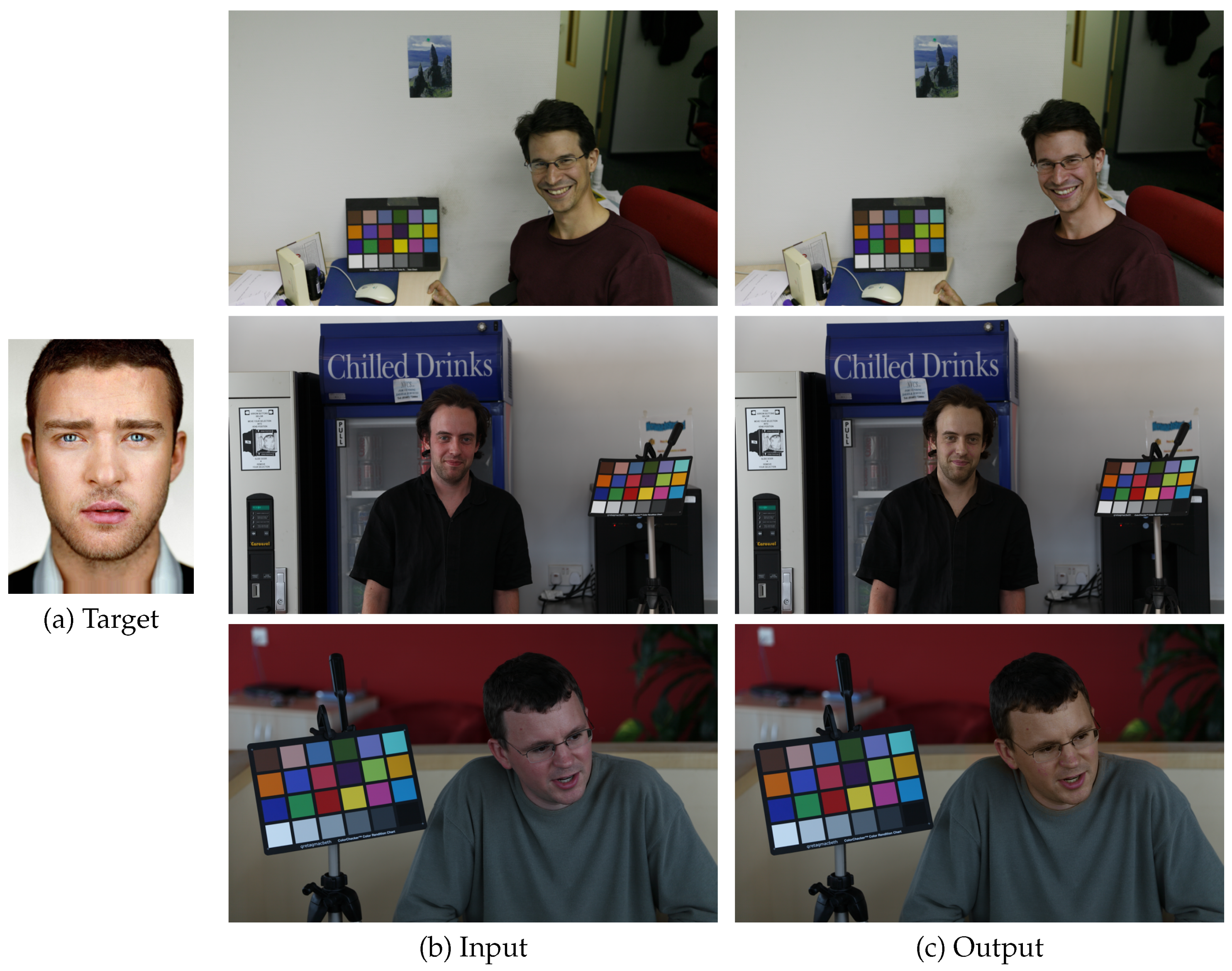
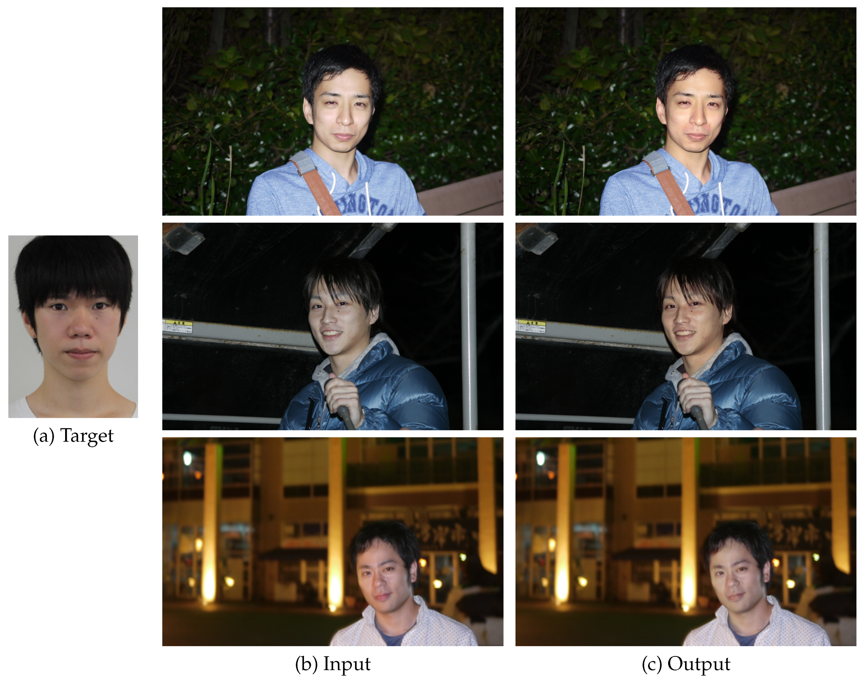
- Each camera has its own camera response sensitivity, producing a different distribution of skin color in a color space.
- Background color is usually reflected to faces causing distorted colors.
- When each subject wears different colored clothes, color correction for the whole image region distorts the skin color, while skin color correction discolors the clothes.
- (1)
- Face detection and Facial skin color extraction;
- (2)
- Facial skin color correction.
2. Related Work
3. Proposed Method
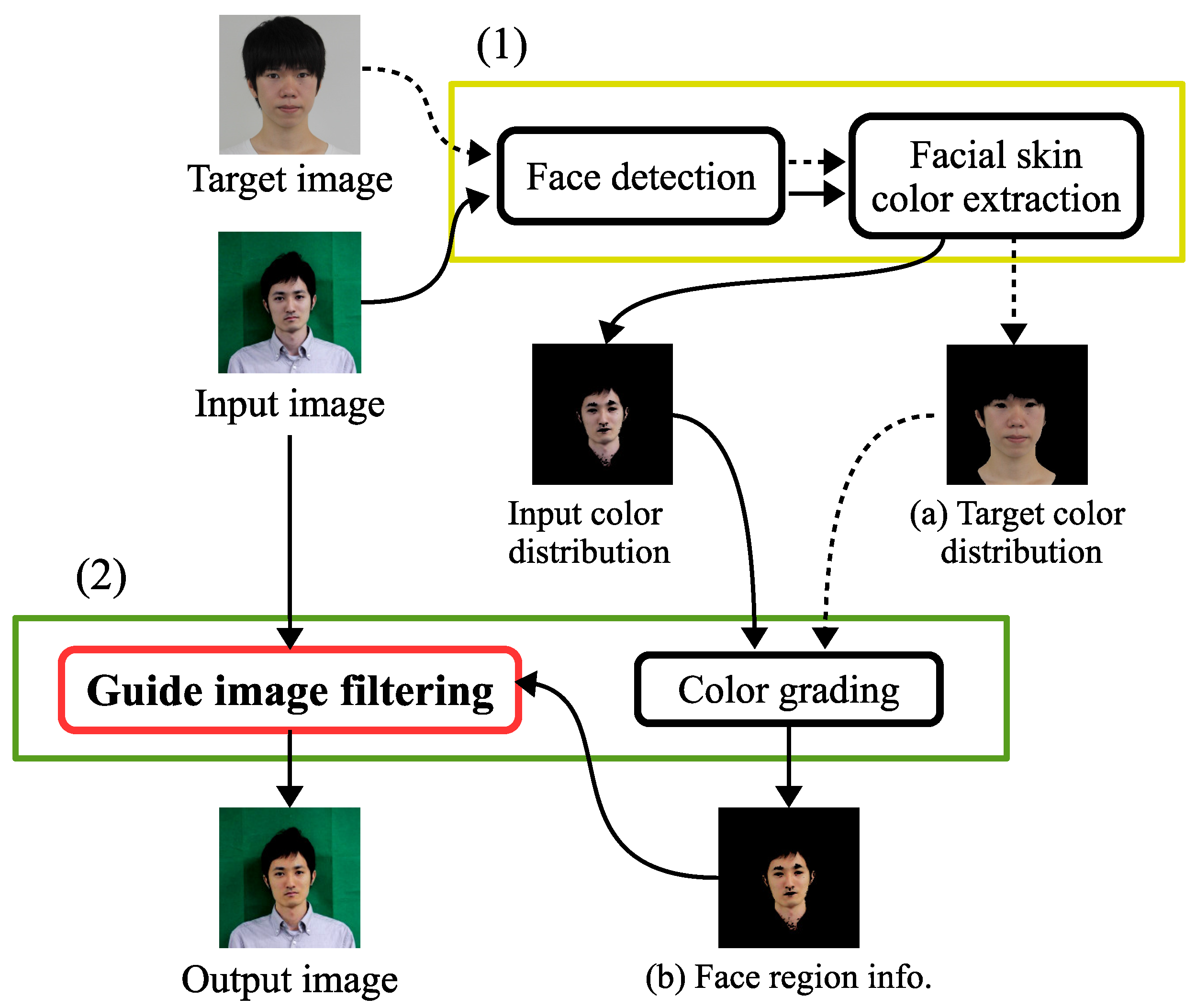
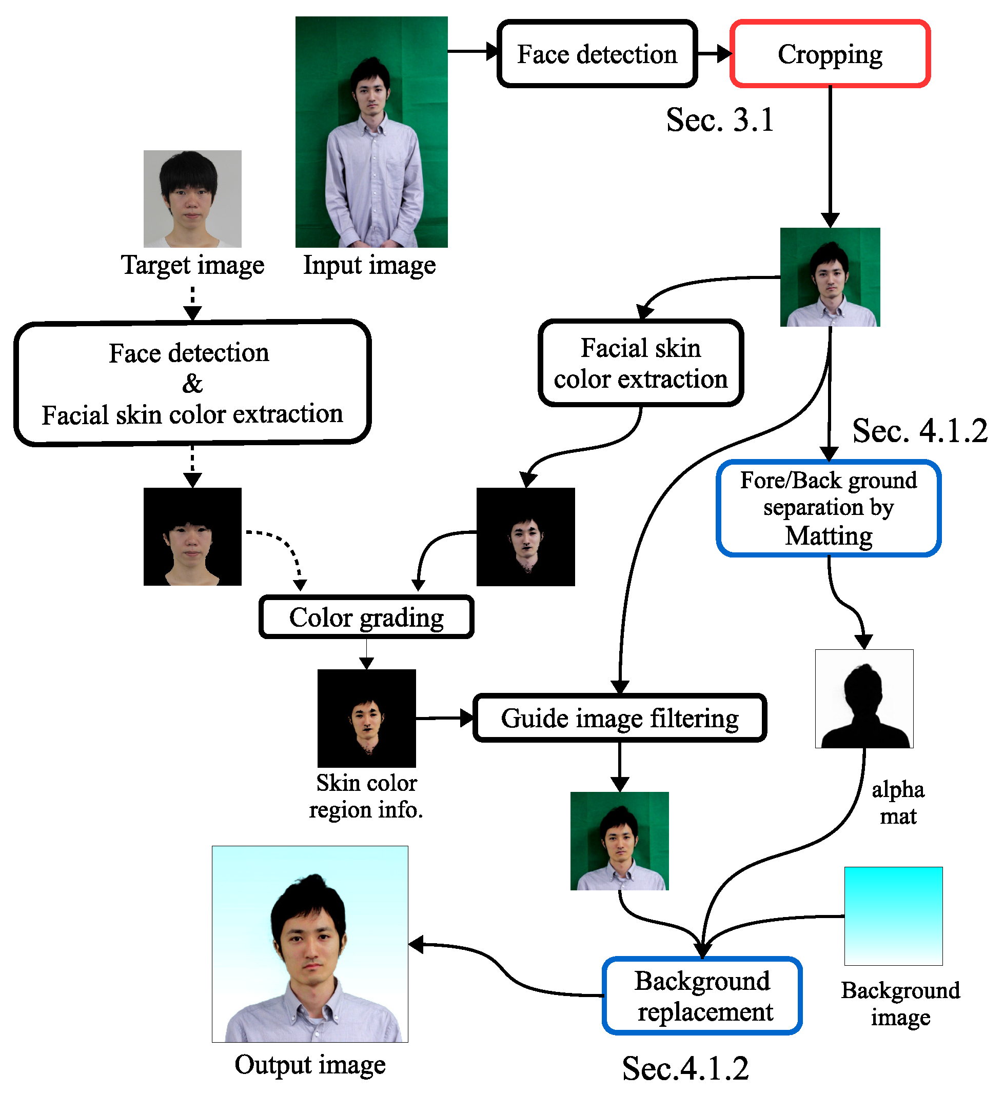
- (1)
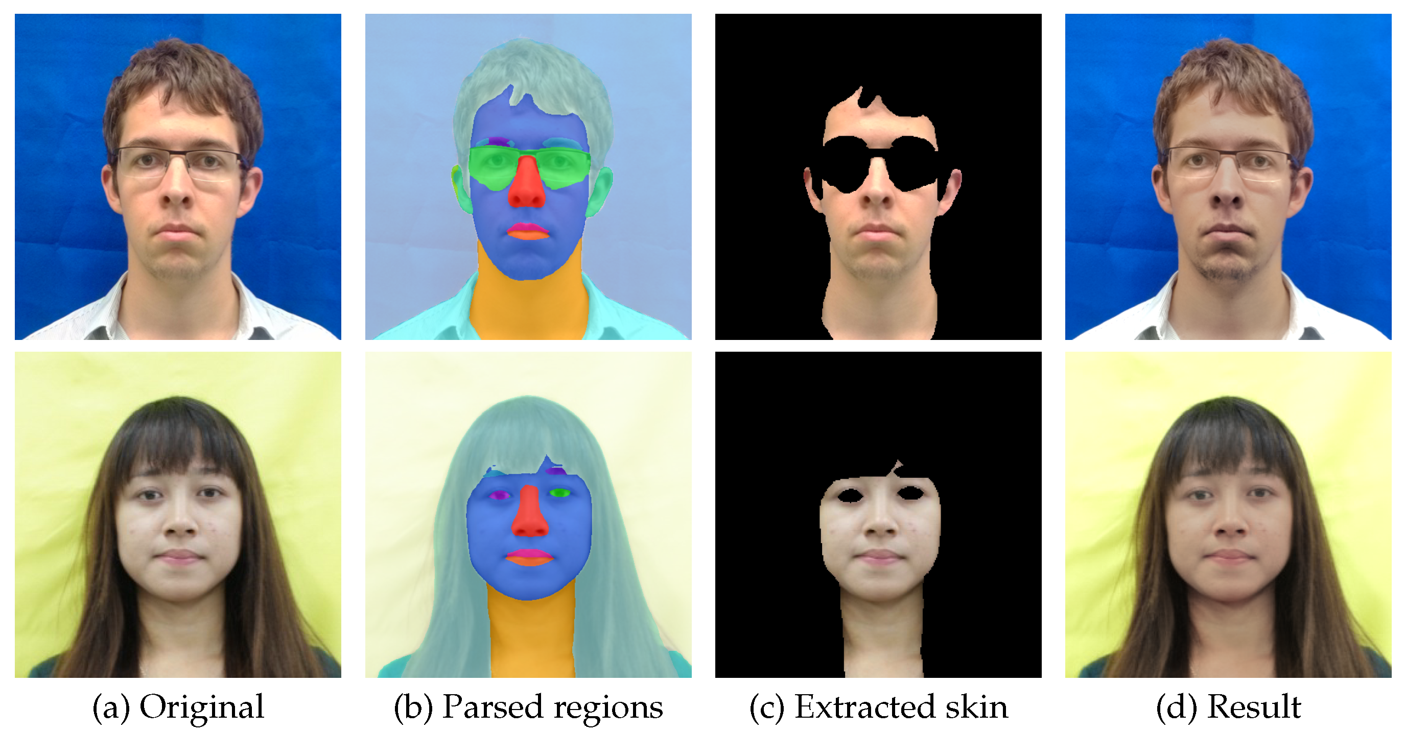
- Face detection and Facial skin color extraction (the yellow box in Figure 1): It detects the face area and extracts its facial skin color.
- (2)
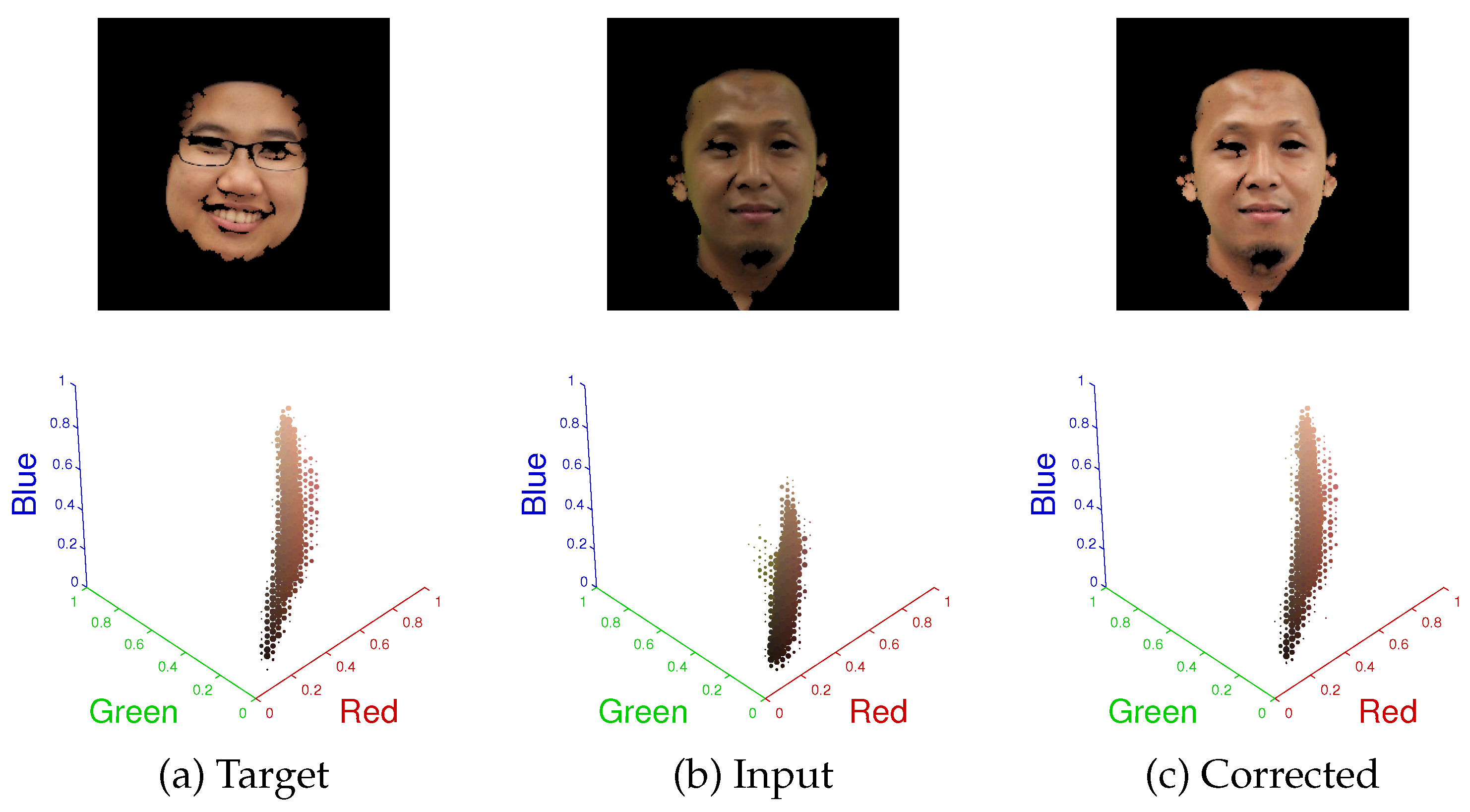
- Skin color correction (green box): The facial skin color extracted is corrected using the target image (a) in the color space. Then, the color of the face region is corrected using the image (b) as the guide image in the image space.
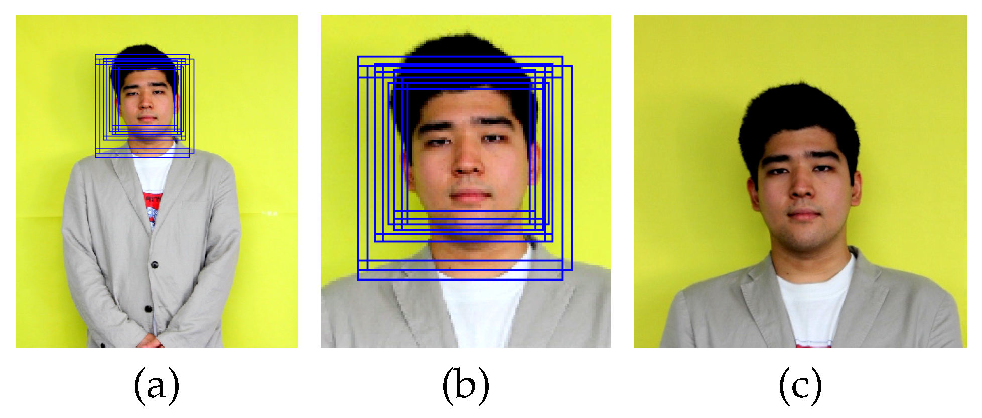
3.1. Face Detection
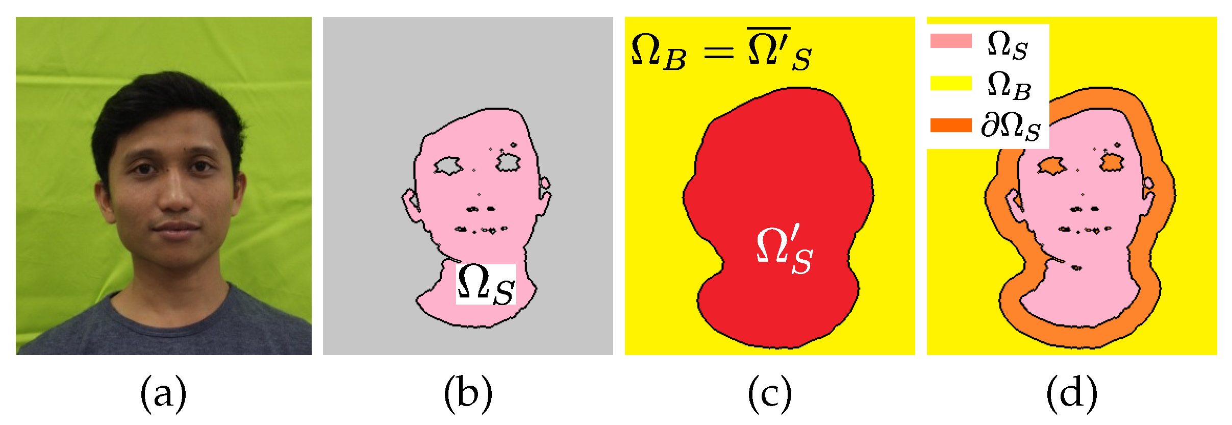
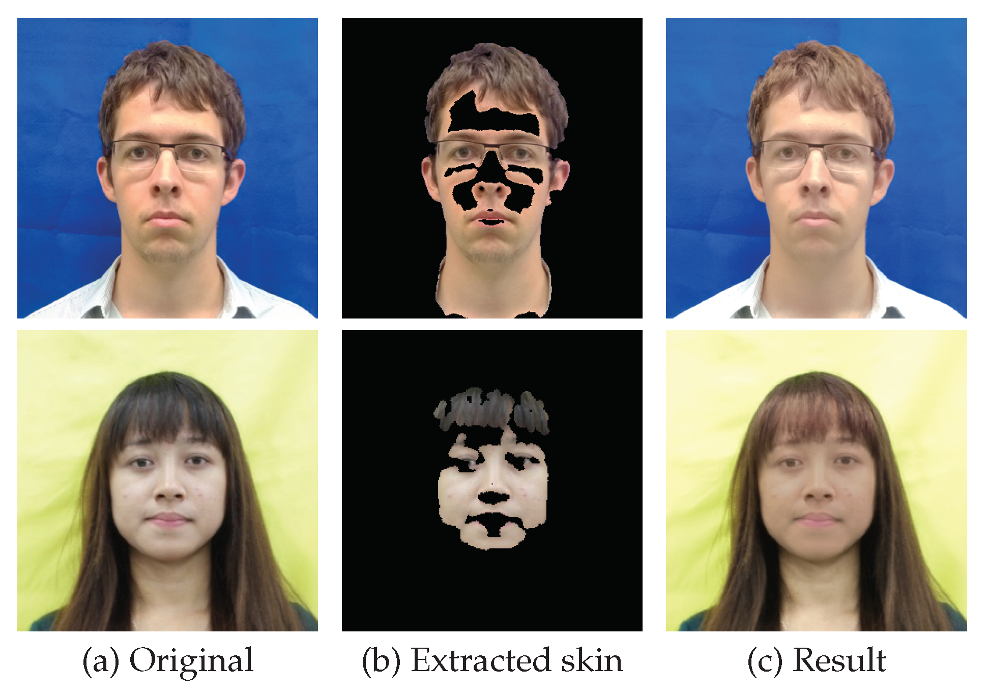
3.2. Skin Color Extraction
- (1)
- The color of each pixel is classified by the color distribution of the entire image in the HSV color space. Each pixel is assigned the label of the cluster to which it belongs.
- (2)
- Some regions are generated by concatenating neighboring pixels with the same labels in the image space. Regions mainly in the detected face area (Equation (2)) are extracted, and regarded as the facial skin region.
3.3. Color Grading
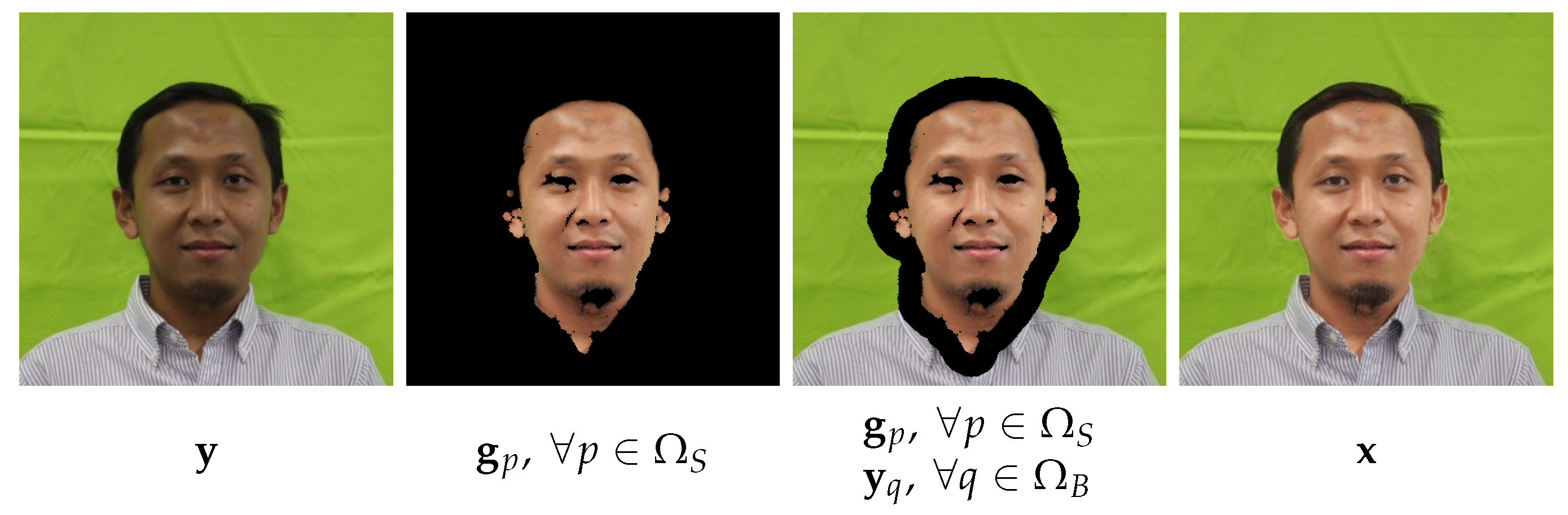
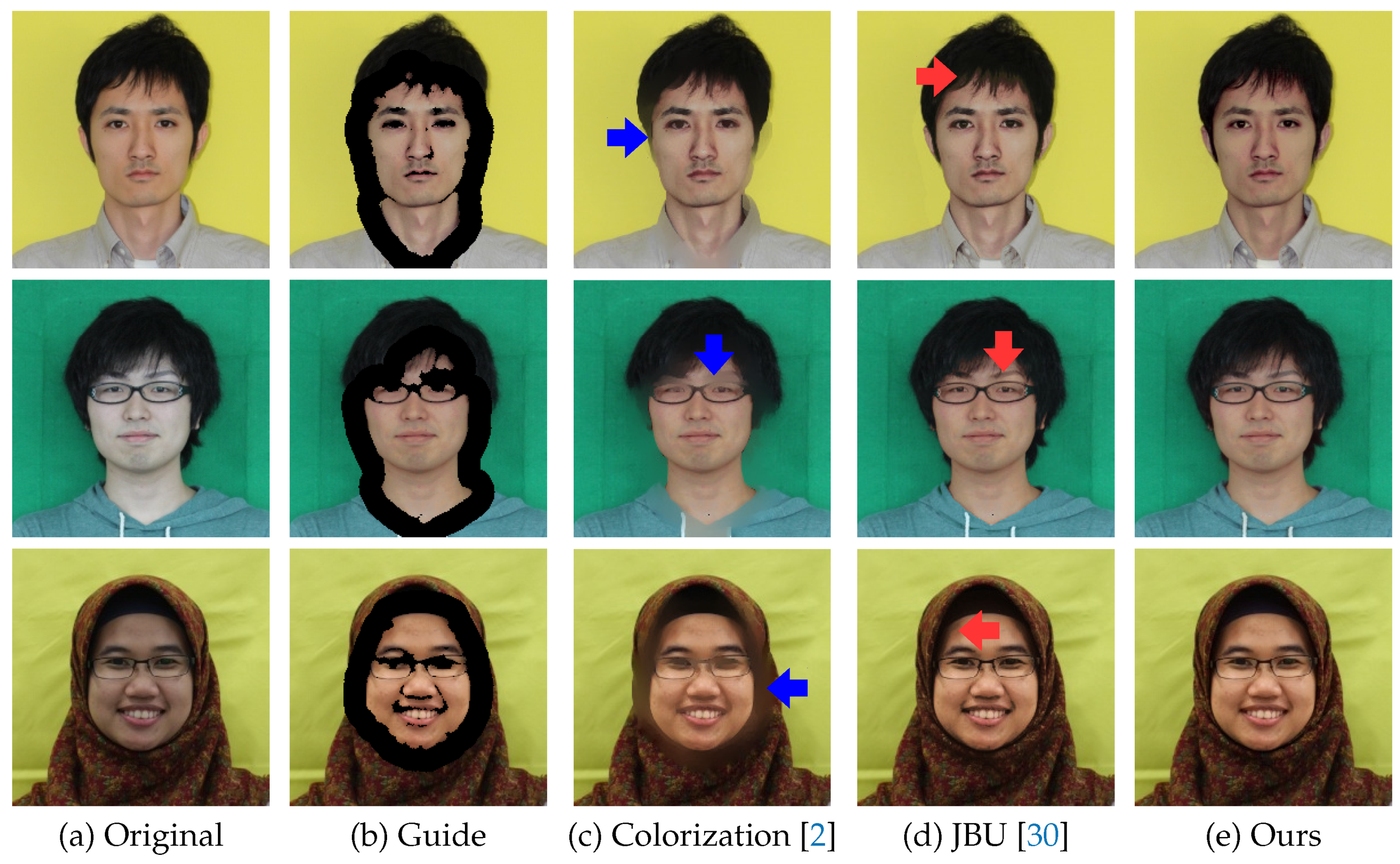
3.4. Guide Image Filtering via Optimization
4. Results and Discussion
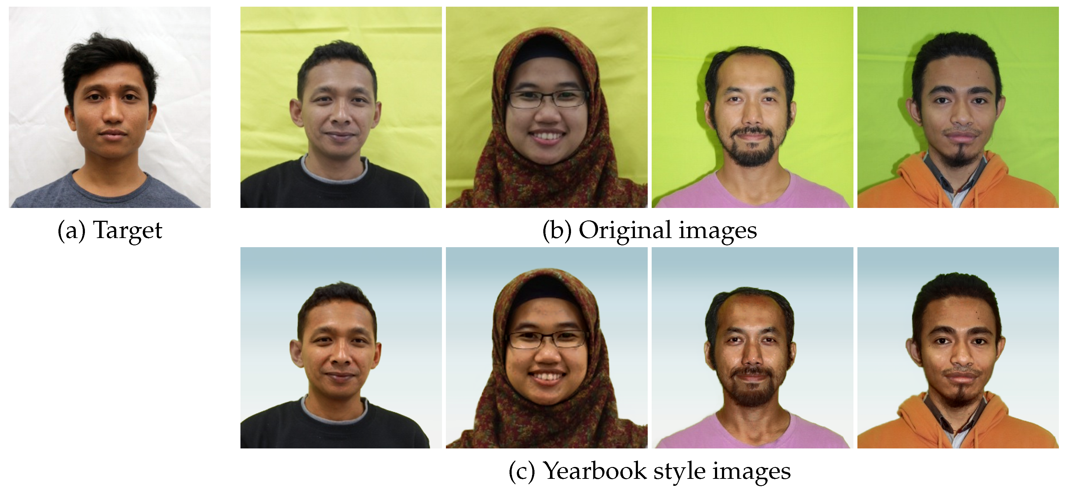
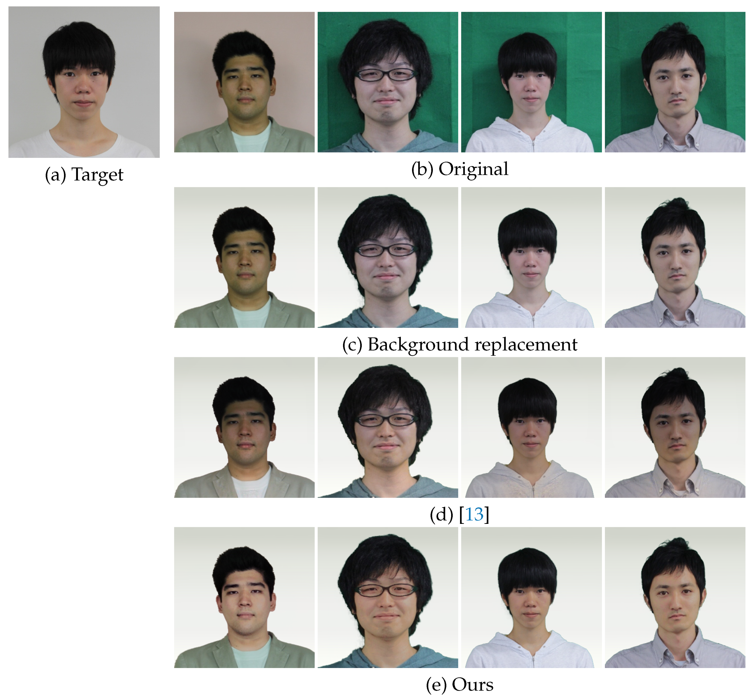
4.1. Automatic Yearbook Style Photo Generation
4.1.1. Face Area Cropping
4.1.2. Background Replacement by Alpha Blending
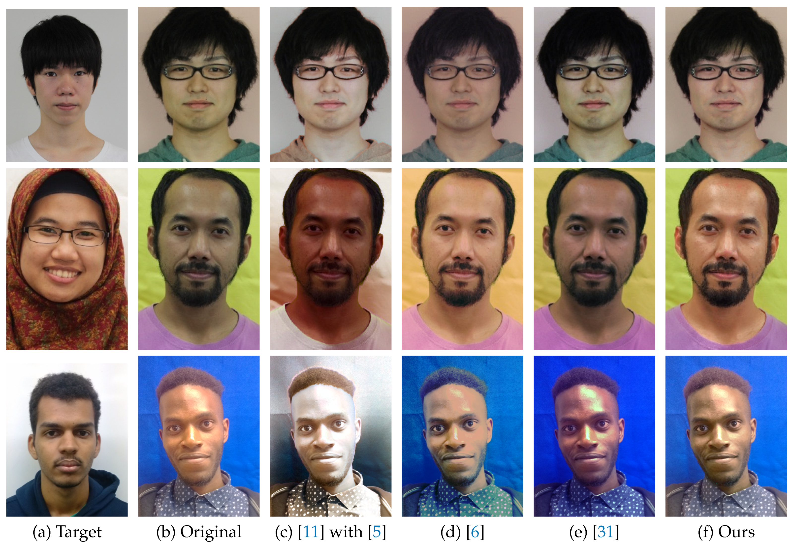
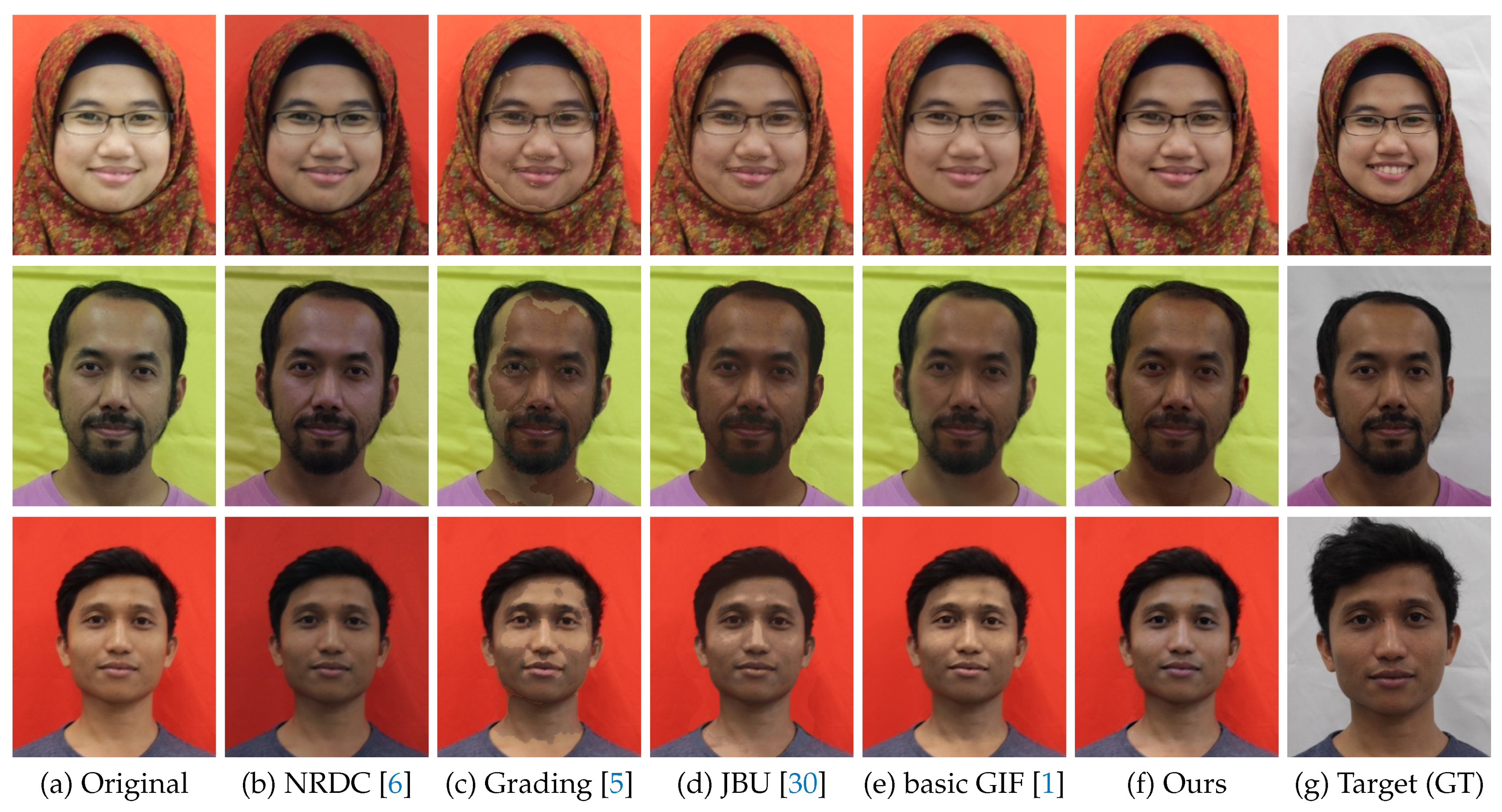
4.2. Comparison with Various Conventional Methods
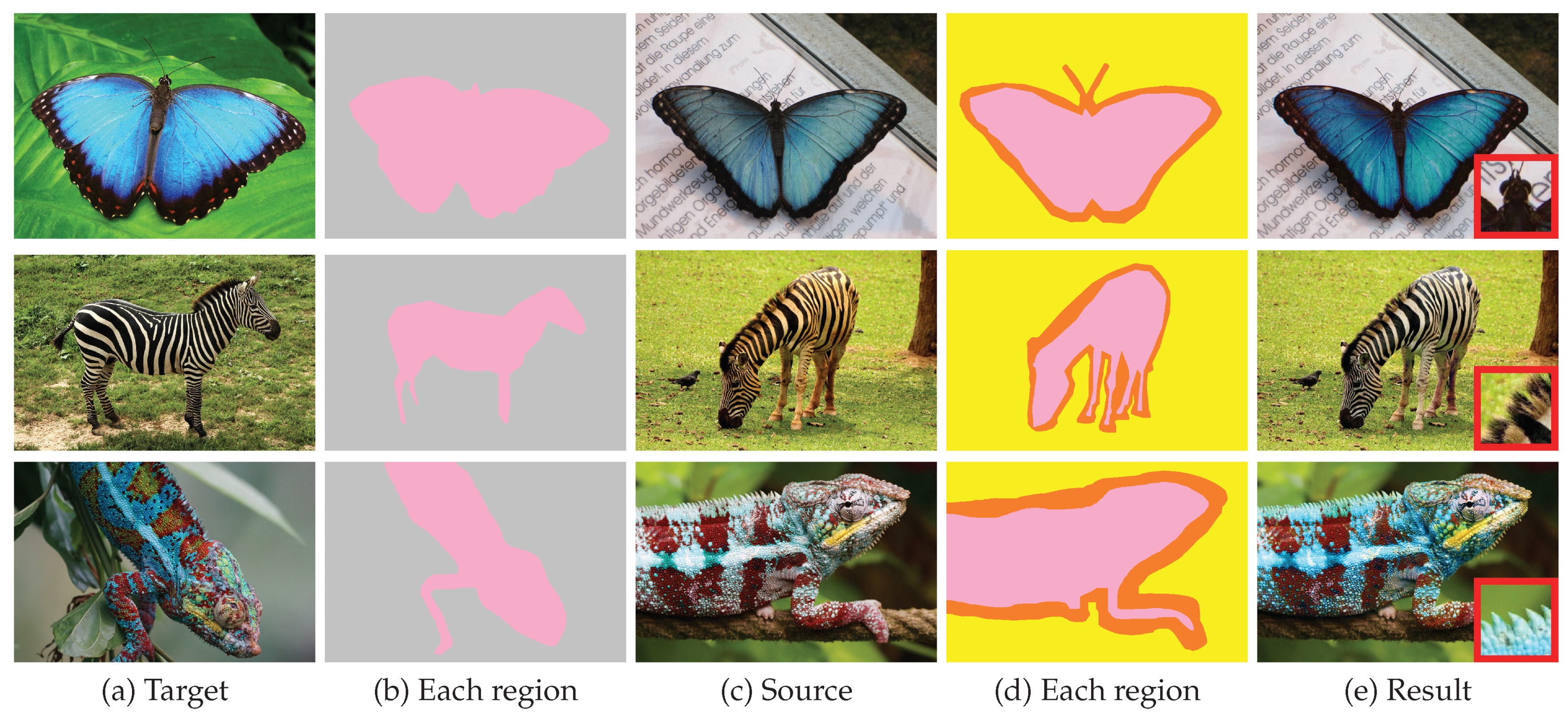
4.3. Semi-Automatic Color Correction
4.4. Limitations
5. Conclusions
Author Contributions
Funding
Institutional Review Board Statement
Informed Consent Statement
Data Availability Statement
Acknowledgments
Conflicts of Interest
Abbreviations
| GIF | Guided image filtering |
| MFIST | Monotone version of the fast iterative shrinkage-thresholding algorithm |
| NRDC | Non-rigid dense correspondence |
| JBU | Joint bilateral upsampling |
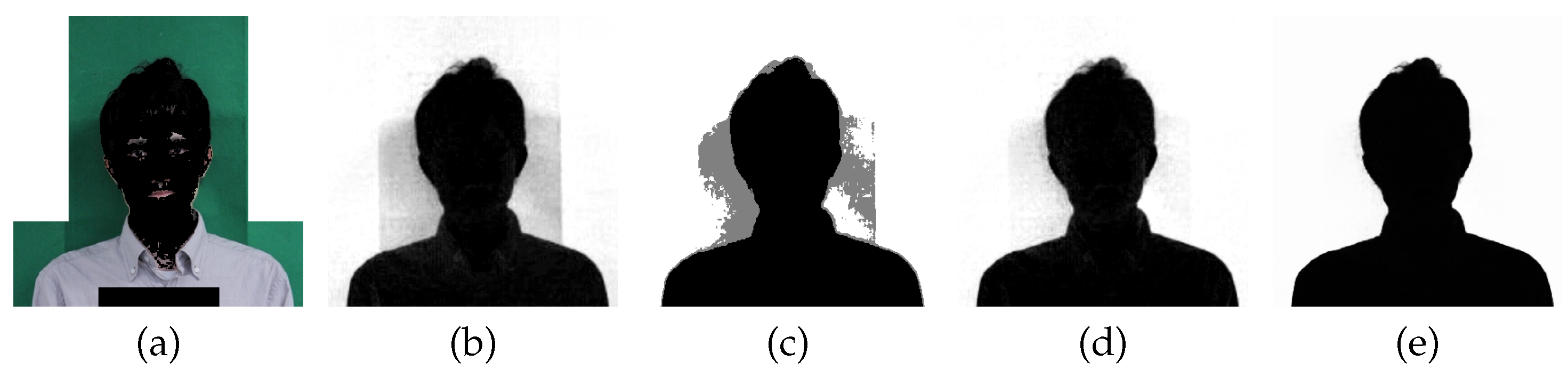
Appendix A. Fore/Background Segmentation by Matting
- (a)
- The initial foreground is the combination of the skin color region and the hair region above the face (we roughly select a black large region). The initial background consists of two rectangular regions on the left and right sides of the face.
- (b)
- Matting [28] is performed, giving a soft label for each pixel.
- (c)
- Region growing in [37] is performed. The group of pixels strongly regarded as background or foreground are, respectively, added to the initial regions and , for the next iteration.
- (d)
- Steps (b) and (c) are repeated a few times (4 times, in our experiment). Additionally, we halve the process window size in matting to implement a coarse-to-fine approach.
- (e)
- A sigmoid function is applied to the alpha-mat as to reduce neutral colors and enhance them to be close to 0 or 1.

References
- He, K.; Sun, J.; Tang, X. Guided image filtering. IEEE Trans. Pattern Anal. Mach. Intell. (TPAMI) 2013, 35, 1397–1409. [Google Scholar] [CrossRef]
- Levin, A.; Lischinski, D.; Weiss, Y. Colorization using Optimization. ACM Trans. Graph. (TOG) 2004, 23, 689–694. [Google Scholar] [CrossRef] [Green Version]
- Levin, A.; Lischinski, D.; Weiss, Y. A Closed-Form Solution to Natural Image Matting. IEEE Trans. Pattern Anal. Mach. Intell. (TPAMI) 2008, 30, 228–242. [Google Scholar] [CrossRef] [Green Version]
- Baba, T.; Perrotin, P.; Tatesumi, Y.; Shirai, K.; Okuda, M. An automatic yearbook style photo generation method using color grading and guide image filtering based facial skin color. In Proceedings of the 2015 3rd IAPR Asian Conference on Pattern Recognition (ACPR), Kuala Lumpur, Malaysia, 3–6 November 2015; pp. 1–6. [Google Scholar]
- Pitié, F.; Kokaram, A.C.; Dahyot, R. Automated colour grading using colour distribution transfer. Comput. Vis. Image Underst. 2007, 107, 123–137. [Google Scholar] [CrossRef]
- HaCohen, Y.; Shechtman, E.; Goldman, D.B.; Lischinski, D. Non-rigid dense correspondence with applications for image enhancement. ACM Trans. Graph. (TOG) 2011, 30, 70:1–70:10. [Google Scholar] [CrossRef]
- HaCohen, Y.; Shechtman, E.; Goldman, D.B.; Lischinski, D. Optimizing color consistency in photo collections. ACM Trans. Graph. (TOG) 2013, 32, 38:1–38:10. [Google Scholar] [CrossRef]
- Qiu, G.; Guan, J. Color by linear neighborhood embedding. In Proceedings of the IEEE International Conference on Image Processing 2005, Genova, Italy, 14 September 2005; Volume 3, pp. 1–4. [Google Scholar]
- Petschnigg, G.; Szeliski, R.; Agrawala, M.; Cohen, M.; Hoppe, H.; Toyama, K. Digital photography with flash and no-flash image pairs. ACM Trans. Graph. (TOG) 2004, 23, 664–672. [Google Scholar] [CrossRef]
- Eisemann, E.; Durand, F. Flash photography enhancement via intrinsic relighting. ACM Trans. Graph. (TOG) 2004, 23, 673–678. [Google Scholar] [CrossRef]
- Rabin, J.; Delon, J.; Gousseau, Y. Regularization of transportation maps for color and contrast transfer. In Proceedings of the 2010 IEEE International Conference on Image Processing, Hong Kong, China, 26–29 September 2010; pp. 1933–1936. [Google Scholar]
- Batool, N.; Chellappa, R. Detection and inpainting of facial wrinkles using texture orientation fields and Markov random field modeling. IEEE Trans. Image Process. (TIP) 2014, 23, 3773–3788. [Google Scholar] [CrossRef] [Green Version]
- Shih, Y.; Paris, S.; Barnes, C.; Freeman, W.T.; Durand, F. Style Transfer for Headshot Portraits. ACM Trans. Graph. (TOG) 2014, 33, 148:1–148:14. [Google Scholar] [CrossRef] [Green Version]
- Viola, P.; Jones, M. Rapid object detection using a boosted cascade of simple features. In Proceedings of the 2001 IEEE Computer Society Conference on Computer Vision and Pattern Recognition, CVPR 2001, Kauai, HI, USA, 8–14 December 2001; Volume 1, pp. I-511–I-518. [Google Scholar]
- King, D.E. Dlib-ml: A Machine Learning Toolkit. J. Mach. Learn. Res. 2009, 10, 1755–1758. [Google Scholar]
- Yu, C.; Wang, J.; Peng, C.; Gao, C.; Yu, G. BiSeNet: Bilateral segmentation network for real-time semantic segmentation. In Computer Vision—ECCV 2018; Springer International Publishing: Cham, Switzerland, 2018; pp. 334–349. [Google Scholar]
- Lloyd, S.P. Least squares quantization in PCM. IEEE Trans. Inf. Theory 1982, 28, 129–137. [Google Scholar] [CrossRef]
- Arthur, D.; Vassilvitskii, S. K-means++: The Advantages of Careful Seeding. In Proceedings of the Annual ACM-SIAM Symp. Discrete Algorithms, New Orleans, Louisiana, 7–9 January 2007; Society for Industrial and Applied Mathematics: Philadelphia, PA, USA, 2007; pp. 1027–1035. [Google Scholar]
- Shan, Q.; Jia, J.; Brown, M.S. Globally optimized linear windowed tone mapping. IEEE Trans. Vis. Comupt. Graph. 2010, 16, 663–675. [Google Scholar] [CrossRef] [PubMed] [Green Version]
- Combettes, P.L.; Pesquet, J.C. Image restoration subject to a total variation constraint. IEEE Trans. Image Process. (TIP) 2004, 13, 1213–1222. [Google Scholar] [CrossRef] [PubMed]
- Fadili, J.M.; Peyré, G. Total variation projection with first order schemes. IEEE Trans. Image Process. (TIP) 2011, 20, 657–669. [Google Scholar] [CrossRef] [PubMed] [Green Version]
- Afonso, M.V.; Bioucas-Dias, J.M.; Figueiredo, M.A.T. An augmented Lagrangian approach to the constrained optimization formulation of imaging inverse problems. IEEE Trans. Image Process. (TIP) 2011, 20, 681–695. [Google Scholar] [CrossRef] [Green Version]
- Teuber, T.; Steidl, G.; Chan, R.H. Minimization and parameter estimation for seminorm regularization models with I-divergence constraints. Inverse Probl. 2013, 29, 035007. [Google Scholar] [CrossRef]
- Ono, S.; Yamada, I. Second-order total generalized variation constraint. In Proceedings of the 2014 IEEE International Conference on Acoustics, Speech and Signal Processing (ICASSP), Florence, Italy, 4–9 May 2014; pp. 4938–4942. [Google Scholar]
- Chierchia, G.; Pustelnik, N.; Pesquet, J.C.; Pesquet-Popescu, B. Epigraphical projection and proximal tools for solving constrained convex optimization problems. Signal Image Video Process. 2015, 9, 1737–1749. [Google Scholar] [CrossRef] [Green Version]
- Ono, S.; Yamada, I. Signal recovery with certain involved convex data-fidelity constraints. IEEE Trans. Signal Process. 2015, 63, 6149–6163. [Google Scholar] [CrossRef]
- Beck, A.; Teboulle, M. Fast gradient-based algorithms for constrained total variation image denoising and deblurring problems. IEEE Trans. Image Process. (TIP) 2009, 18, 2419–2434. [Google Scholar] [CrossRef] [Green Version]
- He, K.; Sun, J.; Tang, X. Fast matting using large kernel matting Laplacian matrices. In Proceedings of the 2010 IEEE Computer Society Conference on Computer Vision and Pattern Recognition, San Francisco, CA, USA, 13–18 June 2010; pp. 2165–2172. [Google Scholar]
- Gehler, P.V.; Rother, C.; Blake, A.; Minka, T.; Sharp, T. Bayesian color constancy revisited. In Proceedings of the 2008 IEEE Conference on Computer Vision and Pattern Recognition, Anchorage, AK, USA, 23–28 June 2008; pp. 1–8. [Google Scholar] [CrossRef]
- Kopf, J.; Cohen, M.F.; Lischinski, D.; Uyttendaele, M. Joint Bilateral Upsampling. ACM Trans. Graph. (TOG) 2007, 26, 96:1–96:5. [Google Scholar] [CrossRef]
- Park, J.; Tai, Y.W.; Sinha, S.; Kweon, I.S. Efficient and Robust Color Consistency for Community Photo Collections. In Proceedings of the 2016 IEEE Conference on Computer Vision and Pattern Recognition (CVPR), Las Vegas, NV, USA, 27–30 June 2016; pp. 430–438. [Google Scholar]
- CoinCheung. Implementatoin of BiSeNetV1 and BiSeNetV2. 2020. Available online: https://github.com/CoinCheung/BiSeNet (accessed on 8 July 2021).
- zll. face-parsing.PyTorch. 2019. Available online: https://github.com/zllrunning/face-parsing.PyTorch (accessed on 8 July 2021).
- Liu, Z.; Luo, P.; Wang, X.; Tang, X. Deep Learning Face Attributes in the Wild. In Proceedings of the International Conference on Computer Vision (ICCV), Santiago, Chile, 7–13 December 2015. [Google Scholar]
- Tai, Y.W.; Jia, J.; Tang, C.K. Soft color segmentation and its applications. IEEE Trans. Pattern Anal. Mach. Intell. (TPAMI) 2007, 29, 1520–1537. [Google Scholar] [CrossRef] [Green Version]
- Aksoy, Y.; Aydin, T.O.; Smolić, A.; Pollefeys, M. Unmixing-based soft color segmentation for image manipulation. ACM Trans. Graph. 2017, 36, 19:1–19:19. [Google Scholar] [CrossRef]
- Sun, J.; Jia, J.; Tang, C.K.; Shum, H.Y. Poisson matting. ACM Trans. Graph. (TOG) 2004, 23, 315–321. [Google Scholar] [CrossRef]


Publisher’s Note: MDPI stays neutral with regard to jurisdictional claims in published maps and institutional affiliations. |
© 2021 by the authors. Licensee MDPI, Basel, Switzerland. This article is an open access article distributed under the terms and conditions of the Creative Commons Attribution (CC BY) license (https://creativecommons.org/licenses/by/4.0/).
Share and Cite
Shirai, K.; Baba, T.; Ono, S.; Okuda, M.; Tatesumi, Y.; Perrotin, P. Guided Facial Skin Color Correction. Signals 2021, 2, 540-558. https://doi.org/10.3390/signals2030033
Shirai K, Baba T, Ono S, Okuda M, Tatesumi Y, Perrotin P. Guided Facial Skin Color Correction. Signals. 2021; 2(3):540-558. https://doi.org/10.3390/signals2030033
Chicago/Turabian StyleShirai, Keiichiro, Tatsuya Baba, Shunsuke Ono, Masahiro Okuda, Yusuke Tatesumi, and Paul Perrotin. 2021. "Guided Facial Skin Color Correction" Signals 2, no. 3: 540-558. https://doi.org/10.3390/signals2030033
APA StyleShirai, K., Baba, T., Ono, S., Okuda, M., Tatesumi, Y., & Perrotin, P. (2021). Guided Facial Skin Color Correction. Signals, 2(3), 540-558. https://doi.org/10.3390/signals2030033