1. Introduction
Multiple passive sensors can be cooperatively used in a target tracking system to achieve target observability. In general, the performance of such a tracking system is correlated with the states of these sensors [
1]. For example, a 2D moving target can be observed by two cooperative bearing-only sensors, while they exhibit observability issues individually [
2]. In this case, the track accuracy is highly dependent on the locations of the sensors when taking measurements. A crucial step in the tracking is to plan the moving sensor trajectories ahead of measurement process in a way which will minimise tracking error at a future time when the measurements taken by the two sensors on the planned trajectories are used [
3,
4].
The sensor trajectory planning problem is also known as trajectory scheduling or optimisation in the literature. It can be cast as a partially observed Markov decision process (POMDP) [
5,
6], where the decision process is carried out by minimising the cost or maximising the reward against a measure criterion that is related to the Fisher information [
7,
8,
9] or mutual information [
10,
11]. Ghassemi and Krishnamurthy describe a method in [
12], where they use a set of orthogonal basis functions, i.e., the Chebychev polynomial series as suggested in [
13] for the control space parameterisation to replace the brute force search for
N-step planning ahead. Logothetis et al. proposed an information theoretic approach to sensor scheduling in [
10]. The sensor is steered so that the mutual information between the posterior density of the target and the measurement sequence at a desired future time is maximized. Practical algorithms for sensor scheduling were discussed in [
11]. Morelande et al. proposed an alternative approach in [
14], which calculates the accumulated reward, defined by the expectation of information divergence between the posterior and prior densities of target, for each possible sensor path and the sensor maneuvers are controlled by the action that maximises the accumulated reward. In general, computing reward functions require the evaluation of future measurements. Of course, it is impossible to give an exact computation of the future reward function since future measurements are inaccessible. One may mitigate this problem by using (conditionally) expected values of the reward at future times, or by using Monte Carlo sampling to numerically evaluate future measurements [
15,
16].
In this paper, we investigate the problem of tracking a moving target via cooperative passive sensors, where the tracking error is a function of sensor trajectories. The focus is on two statistical reward functions for passive sensing, both available in the analytic form. They are referred to as the Expected Rényi information divergence (RID) and the determinant of the Fisher information matrix (FIM). Being available analytically, they are potentially useful for a longer horizon sensor trajectory planning, even on the platforms with limited computational resources. The paper investigates the implications of the approximations involved in derivation of the two reward functions. The analytic expression for the Expected RID is derived assuming a linear-Gaussian case. We show that this approximation significantly reduces the cross-correlation of the tracking error between the two sensor locations, and consequently results in the performance similar to that of the trace of the FIM. On the other hand, the determinant of FIM, where the ground truth is approximated by the prediction of the target state, taking correctly into account the cross-correlation between the two sensors. We also discuss this problem from the information geometric viewpoint by illustrating the geometric properties of the FIM corresponding to the statistical reward function. Finally, we compare the performance of the two reward functions by a numerical example in which a (non-cooperative) target is being chased by two cooperative bearing-only sensors. Preliminary work on this subject was reported in [
17].
The paper is organised as follows: the sensor trajectory scheduling problem of interest is described in
Section 2. The analytic expressions for the two reward functions, i.e., the Expected RID and the determinant of FIM are derived and their performance discussed in
Section 3. In
Section 4, we further compare the performance difference between the two reward functions from the information geometric viewpoint. Simulation results are presented in
Section 5. Finally, the concluding remarks are given in
Section 7.
2. Problem Definition
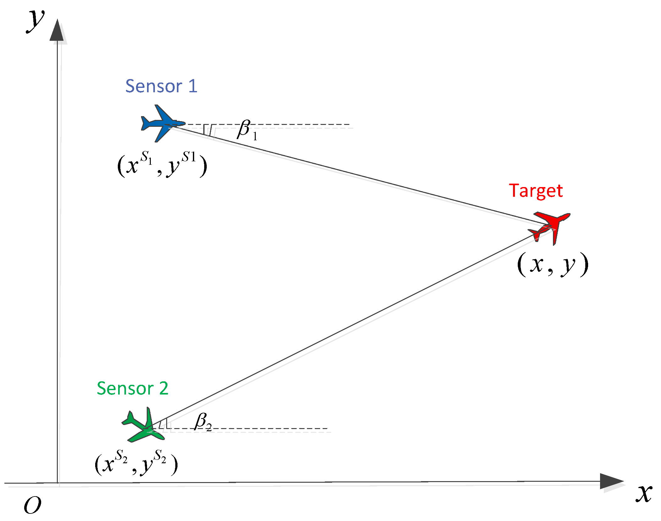
Let us consider the problem of two-dimensional target tracking using measurements from two cooperative bearing-only sensors as shown in
Figure 1.
The target state, which consists of both target location
and velocity
, at time
is
The system and measurement models are
where the system transition matrix is
and
and
are system and measurement noises, respectively. These are assumed to be independent Gaussian distributions, that is,
where
is assumed to be known and
and
are the standard deviations of measurement noises for sensors 1 and sensor 2, respectively.
The measurement function in (
2) is expressed as
where
and
are the locations of sensor 1 and sensor 2 at
, respectively.
The objective of target tracking is to estimate the target posterior probability density function (PDF)
based on the bearings-only measurement sequence
up to current time
and the prior PDF
. Clearly, the measurement model (
4) is sensor state dependent, and so tracking accuracy depends on where the two sensors take measurements (i.e., on their motion). Our goal is to find the optimal future motion for the two sensors within the limitations imposed by the sensor platform dynamics, so as to minimize the future expected track error. This is a difficult problem because of the many sources of uncertainty involved in decision-making: the uncertainty in the current target state estimate as well as the uncertainty in the future target motion and measurements.
A practical way to implement the sensor trajectory optimisation procedure is to assume that sensor platforms move at constant speeds,
and
, respectively, and that they have a small set
of admissible course corrections at time
. Each element
of
is a pair
, where
represents the course correction of the
ith sensor at
k. This results in the velocities of the two sensors in the local coordinates in the time interval
as
The assumption of constant speeds between sampling intervals is a standard practice for system analysis of discrete data sampling without loss of optimality. The analysis tends to be optimal at a high sampling rate.
In summary, the underlying target tracking is a POMDP and involves an
N-step ahead process of sensor trajectory planning, which computes the optimal action sequence
such that the tracking error is minimised at the future time
. A generic recursive process of sensor trajectory scheduling and target state estimation at discrete-time
involves the steps listed in Algorithm 1:
| Algorithm 1 Sensor scheduling steps at discrete-time k |
- 1:
Inputs: The posterior at k, ; the sensor locations and course corrections . - 2:
Propose the set of admissible sensor actions - 3:
Perform scheduling based on an optimality criterion and obtain the optimal sequence of future sensor actions for a future time period . - 4:
Steer each sensor to the computed location at speed and course correction . - 5:
Take (bearings-only) measurements at time and then compute the posterior PDF of target via a suitable tracker. - 6:
Outputs:; and .
|
3. Reward Functions
The sensor trajectory scheduling is part of the underlying target tracking process, involving the computation of a sequence of future actions (sensor course corrections) based on the current target and sensor states. The key role in this process plays the criterion for measuring the reward of the future action. The reward functions used in the literature are based on the information theoretic measures. One criterion is the mutual information between the posterior probability density of the estimated target state and the measurement sequence, which we seek to maximize. A theoretic description is given in [
18] and sub-optimal strategies are discussed in [
19]. An alternative criterion is to maximize the information divergence between the prior and posterior probability densities of estimated target state [
14]. As the ultimate goal of sensor trajectory optimisation is to improve target tracking accuracy, the posterior Cramer–Rao low bound [
20] is also used as a cost function to take the estimator performance into account as well. In addition, we can also maximize the determinant or trace of the FIM [
13]. All of these criteria are consistent in the sense that they maximize the Fisher information of the underlying system.
In this work, we investigate two reward functions for the problem at hand, which can be derived analytically: the Expected RID and the Determinant of the FIM. For the purpose of comparison, we also introduce the reward function based on the Trace of the FIM. The goal is to find a reward function which is both computationally efficient and reflects correctly the information change associated with various sensor trajectory hypotheses.
3.1. Expected RID
The Rényi information divergence [
21] is the information divergence for probability densities
and
, for
,
For the underlying system with one-step ahead sensor scheduling,
signifies the posterior density at
and
signifies the predicted density at
, where
is the future measurement at time
given by (
2). Thus, (
6) becomes
The evaluation of the integral (
7) requires the future measurement
, which may be obtained numerically via Monte Carlo simulations [
15,
16]. A statistical solution in a closed-form can be derived for the linear Gaussian case [
14], where the dependence on the future measurement
is removed by taking the expectation w.r.t.
.
The linear Gaussian case is described by the transition
and measurement
The predicted measurement distribution is then given by
where
.
Assume that the sequence of measurements
has been collected so that the posterior density is given by
where
is the updated covariance at
k.
For the properties of the Kalman filter, the divergence between the prior PDF and posterior PDF at
is given by
Taking the expectation of (
12) with respect to
and using the formula
we obtain the closed-form Expected RID function [
22]:
where
and
is the covariance matrix associated with the predicted state estimate
.
For the bearings-only problem described in
Section 2, see Equations (
1) and (
2), the Expected RID can only be approximated via linearisation, i.e.,
in (
14) is replaced by the Jacobian of (
4)
Note that
is obtained from the underlying tracker [
23] and
is replaced by
associated with (
2).
3.2. Determinant of Fisher Information Matrix
In general, it is non-trivial to derive the FIM or its determinant in a closed-form. For this particular case, the measurement model (
4) is independent of target velocity and the resulting FIM is only of rank 2. In consequence, we only need to consider the target position components in derivation of the FIM, and therefore the target state vector
in derivation will denote just the target position components (
). A closed form expression for the determinant of the FIM is analytically tractable as follows.
Suppose that the posterior at
is
. Using the current sensor locations and a proposed action
, one can compute the one-step ahead sensor locations
for
. The FIM
at time
for the measurement (
2) is defined to be
where
is the log-likelihood, which is obtained from Equation (
2), and
is a
matrix with entries
Under the Gaussian measurement noise assumption, we have
The determinant of
is a function of
and
. From the definition and using (
19)–(
21), we have
Calculation of the FIM requires knowledge of the target location at future time
k, which in practice is approximated using the predicted target state
based on the point estimate from
and the system dynamics (
1).
3.3. Trace of Fisher Information Matrix
In view of (
19)–(
21), the trace of the FIM is given by
The trace of the FIM is a widely used objective function for sensor information maximisation [
24], but it is more conservative than the determinant of the FIM since it does not take into account the off-diagonal terms of FIM. It will be used to explain the behaviour of the Expected RID function.
3.4. Remarks on the Reward Functions
Both the Expected RID and the Determinant of FIM involve approximations: the former using linearisation, the latter using the predicted target state in place of the true state. The following analysis highlights the difference between the two reward functions after approximation.
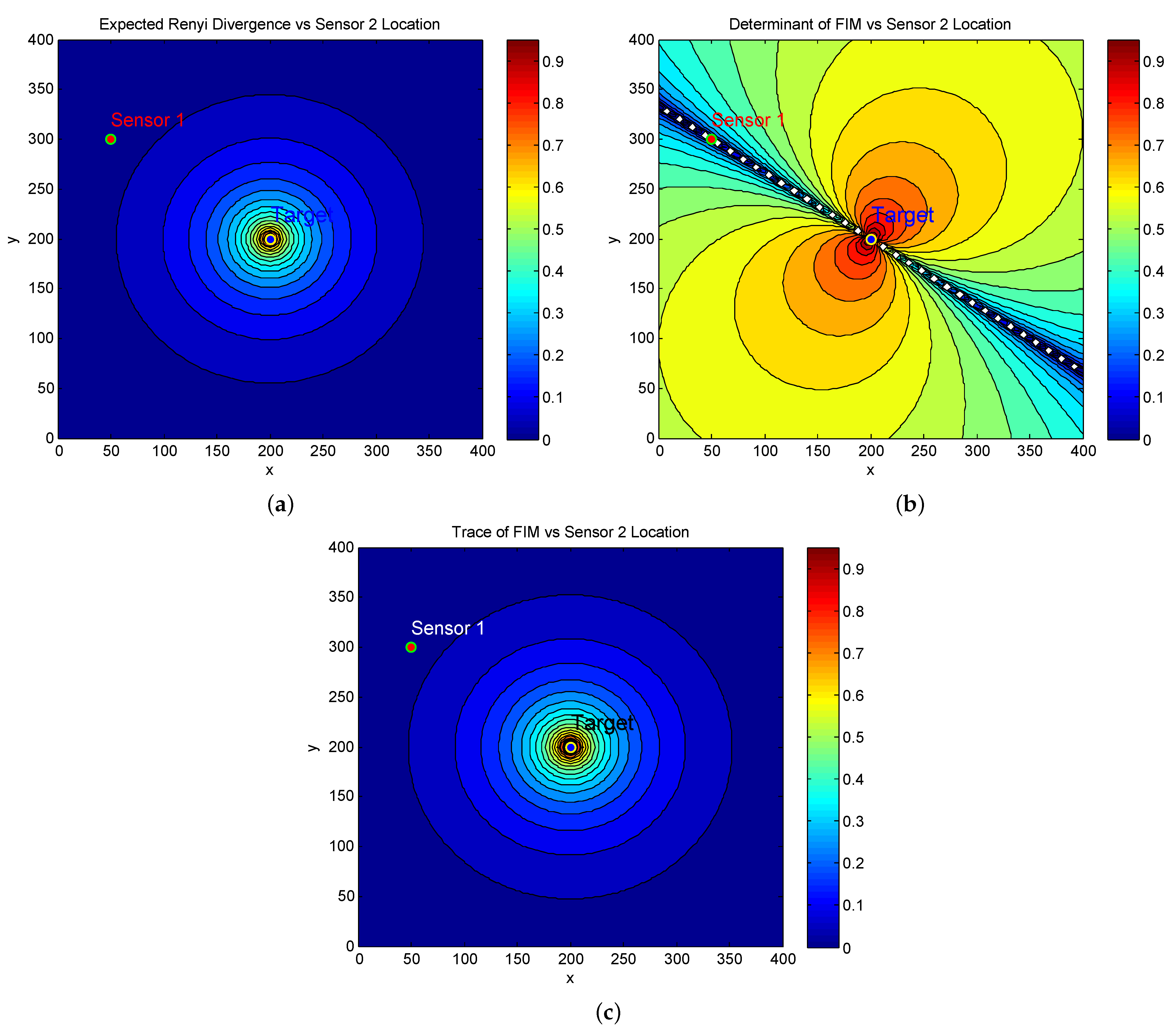
To compare the performance difference of the reward functions, we fix the location of Sensor 1 at
, and plot the reward of one step ahead versus the location of Sensor 2. In the simulation,
is set to be a constant,
(rad) and
(rad). The contour plots for the Expected RID and Determinant of FIM are in
Figure 2a,b, respectively.
In view of these figures, we can make the following observations:
While
Figure 2a shows an increasing reward as Sensor 2 approaches the target, there is no information change observed when Sensor 2 moves around the target in a circle. This indicates that the Expected RID changes only with respect to the distance from individual sensors to the target rather than with respect to the relative locations of the two sensors. This is in contrast to the value of the Determinant of FIM shown in
Figure 2b.
Figure 2b shows a straight line across the two sensor locations, where the values of FIM are singular. This indicates a subspace corresponding to the singular points on which the target state is unobservable. On the other hand, neither the expected RID nor the trace of the FIM take this singular subspace into account.
We observed that the contour plot of the Expected RID in
Figure 2a is virtually the same as that of the Trace of FIM shown in
Figure 2c. The latter is independent of the two sensor locations as long as their distances to the target remain unchanged and this is verified by (
23). This suggests that the Expected RID does not preserve the observed information structure with respect to the two sensor locations after linearisation.
Note that we fix the location of sensor 1 in
Figure 2 for a clear visualization of the difference in comparison, given that both sensors are movable in the sensor trajectory optimisation.
4. Geometric Interpretation on Reward Function
The above argument on the selection of a reward function in cooperative sensing can be described using information geometry. It is well known that the FIM can be used as a metric tensor defining a Riemannian manifold, called the statistical manifold [
25]. Riemannian geometrical concepts, thereby, can inform in problems such as ours. For instance, the Fisher Information distance, defined in terms of the Riemannian metric, can be used to compare parameterised distributions.
For the problem at hand, the family of probability distributions
, parameterised in the target location space
, forms a 2D statistical manifold where
plays the role of a coordinate system of
S. The Fisher information distance (FID) between
and
is defined as the integral along the curve
:
where the minimizing curve is a geodesic in the Riemannian manifold. In local coordinates, the geodesic equations are given by the Euler–Lagrange equations as [
25]
For convenience, we use the subscript
i of
to represent its
ith component and thus
are the coordinates of the curve
,
are the
Christoffel symbols of the second kind, and we can use the Levi–Civita connection coefficients,
where
signifies the inverse of
and Einstein notation for summation is used.
The geodesic equations in (
25) are ordinary differential equations for the coordinates
. A unique solution
can be found for given initial conditions
and
, which is analogous to an initial position
and the “speed”
in the sense of the classical mechanics, where
denotes the tangent vector of
S at
.
Assume that a geodesic is projected onto the parameter space
with a starting point
and a tangent vector
. The exponential map of the starting point is then defined as [
26]
where the notation
is used to signify a geodesic with a starting point
, a tangent vector
and end point
.
It can be shown that the length along the geodesic between
and
is
[
26,
27]. Thus, for a fixed
, the plot of geodesics along all directions at
produces an FID circle centered at
in
S. Intuitively, the projection of an equal FID circle from statistical manifold to the parameter space, which is generally not isotropic in magnitude, reflects the observability of the underlying sensors at given states. With the FIM corresponding to a sensible reward function, the projection will vary as the state of a sensor changes.
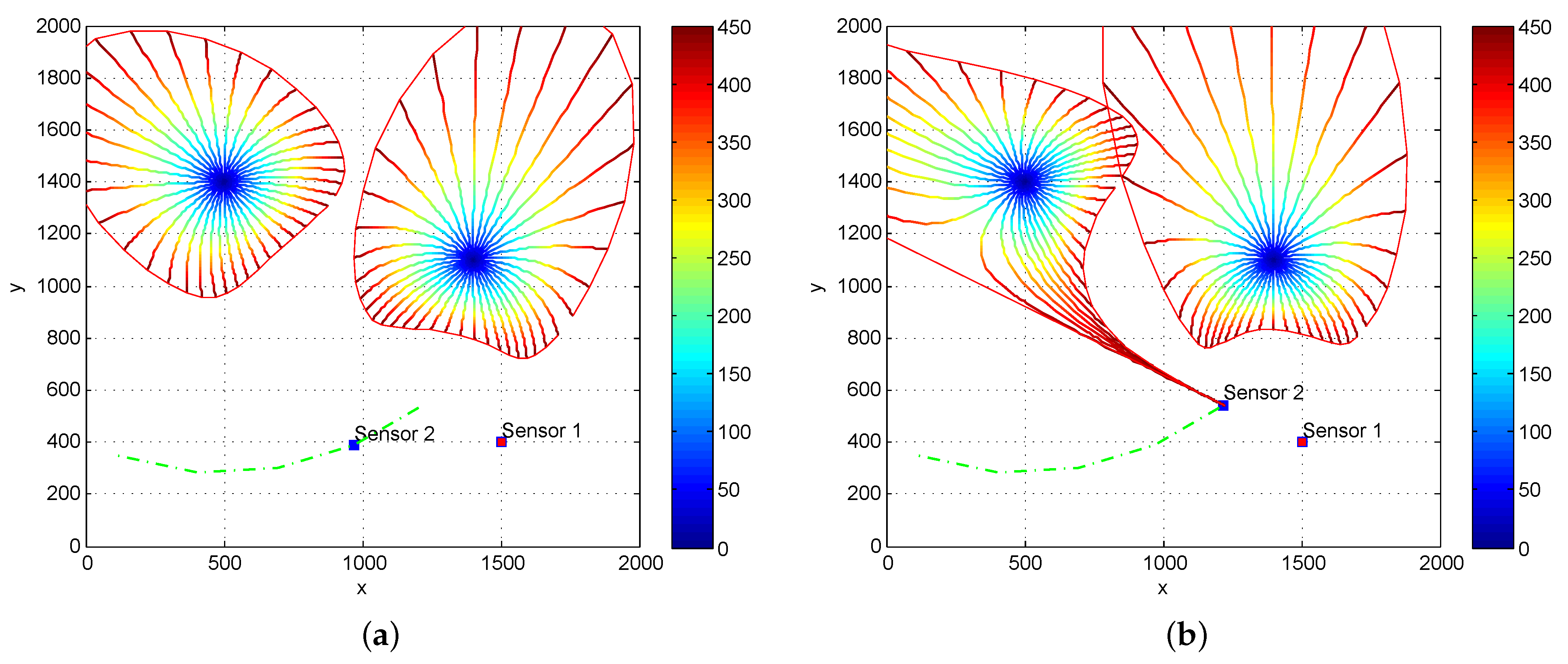
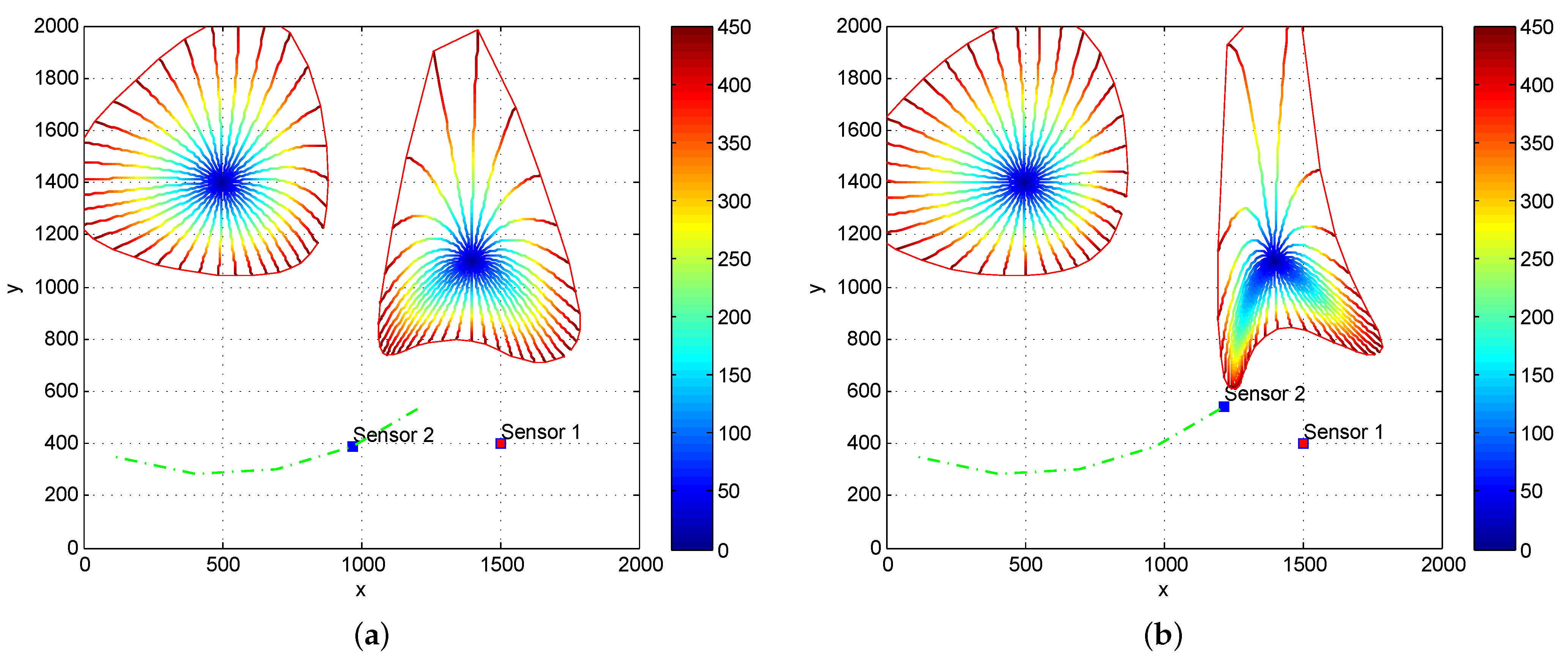
To highlight the difference between the two statistical reward functions in question, we plot the projection of FID circles in parameter space under the scenario where two fixed targets are observed by the two bearing-only sensors. These circles are centred at a target state with the same radius in the statistical manifold spanned by the FIM corresponding to the two statistical reward functions, respectively.
We examine the changes of FID circles before and after the Sensor 2 move circularly around one target.
The FID circles, shown in
Figure 3a,b, have changed significantly as Sensor 2 moves circularly around the target on the left. This indicates that the amount of target information which may be observed by the two sensors varies with sensor states. On the other hand, if we plot the FID circles in the statistical manifold spanned by the FIM without off-diagonal elements which correspond to using the trace of FIM as a statistical reward function, as shown in
Figure 4a,b, the FID circle centered at the target on the left does not change as the Sensor 2 moves circularly around the target.
We emphasize that sensor 2 moves close to the target on the right while keeping the same distance to the target on the left. The FID circles on both left and right targets change in
Figure 3 under the Determinant of FIM, but the FID circle on the left remains the same as shown in
Figure 4 after the movement of sensor 2 when the Trace of FIM criterion is used. This result indicates that the Fisher information will not be fully explored if trace rather than determinant of the FIM is used as a statistical reward function. The Expected RID performs similarly to the trace of FIM.
5. Simulation Example
In this section, we illustrate the effectiveness of sensor scheduling using an example of tracking a maneuvering target by two bearing-only sensors. Target motion follows a hidden Markov process which contains the states of a left turn (), a right turn () and straightline (), and it is moving at a constant speed of 10 m/s. The initial target state is In the first 50 of a total of 100 scans, the target is in the left turn state and it shifts to a right turn state for the rest of scans. Initially, the two bearing-only sensors are moving at a constant speed of 10m/s from the locations m and m heading in the directions and , respectively. They acquire bearing measurements of the target at a sampling rate of T = 5 s. During each scan, they will be steered to one of five directions with respect to their current headings according to the trajectory optimisation decision. The 5 directions are , and .
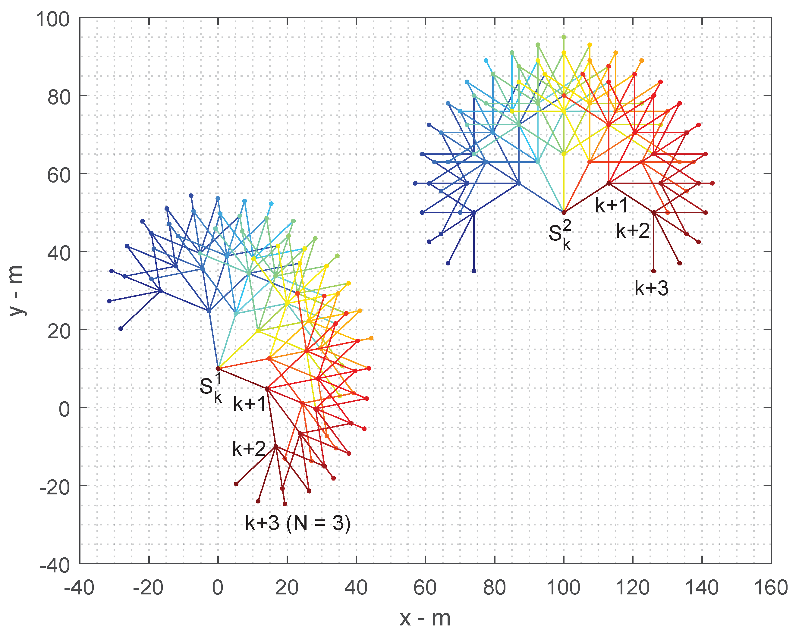
Therefore, for a
N-Step ahead decision process, the number of action hypotheses yielded for the two cooperative sensors are
. For example, the number of action hypotheses for
is
and for
is
. We illustrate this example in
Figure 5.
In practice, the maximum number of hypothesis histories allowed to steer future measurement at each epoch is constrained by a fixed number “MaxH” to provide a feasible computational overhead for real-time operation. In our simulation, we set MaxH = 1000 and such a choice does not affect the comparison of the optimisation performance under different reward functions. We observed from simulation that under this constraint the track error difference between and is statistically close to zero and thus is negligible. Therefore, in the performance comparison versus Monte Carlo runs, we only consider .
An EKF tracker [
28] is implemented to estimate the posterior density of target state from the target bearing measurements taken by the two sensors. We assume that the target bearing measurements are corrupted with a Gaussian noise of zero-mean with standard deviation of two degrees.
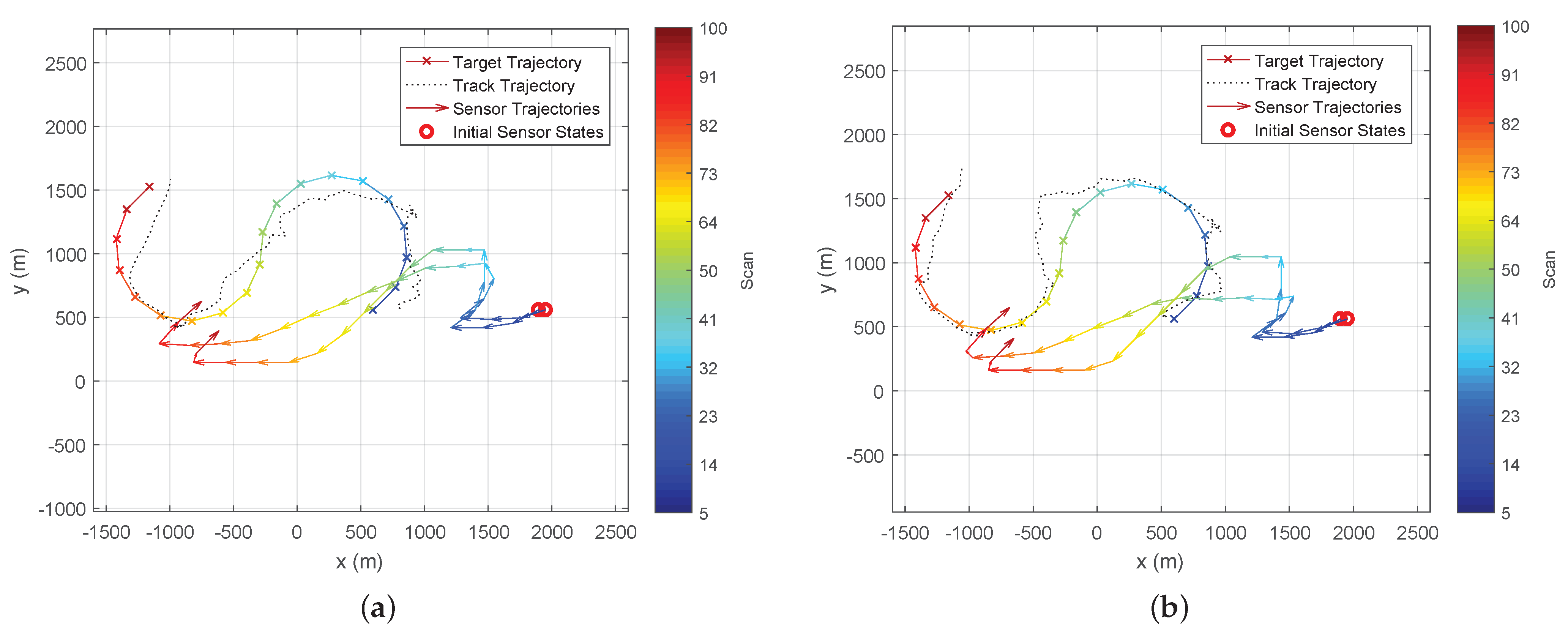
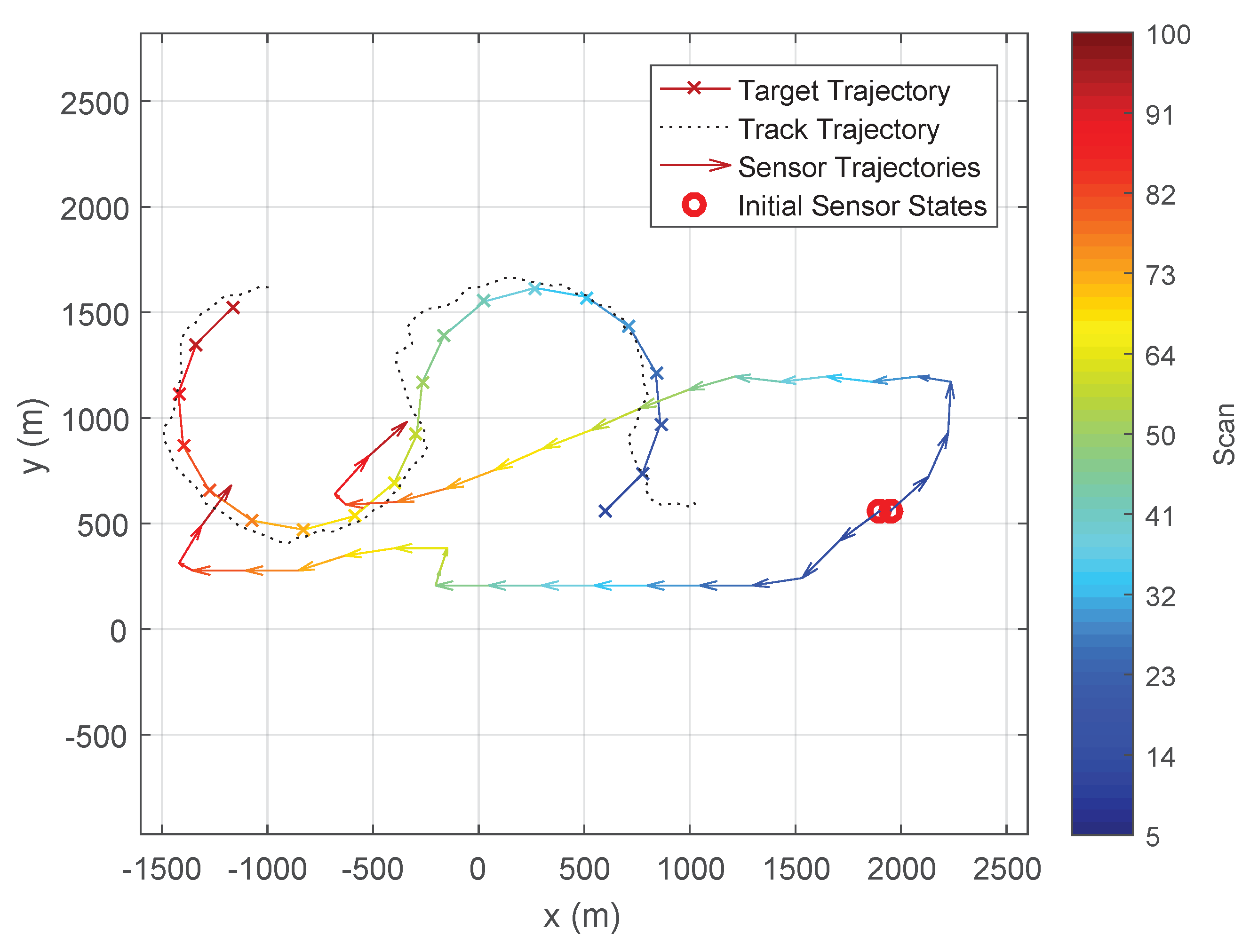
Figure 6 and
Figure 7 show the typical trajectories of the two bearing-only sensors in the target tracking experiment under the Determinant of FIM (DetFIM), the Expected RID (ExpReward), and the Trace of FIM (TrFIM), respectively. By maximising DetFIM, the two sensors move in a way such that the angle formed by sensor 1, target, sensor 2 is approximately
while approaching the target. Thus, the measurements taken by the two sensors along these computed trajectories minimise the error covariance of the underlying tracker (
Figure 6). On the other hand, the sensor trajectories scheduled by maximising ExpReward (or TrFIM) show no cooperative movement between the sensors while they are approaching the target. This is because none of correlations between the two sensors with respect to the target are used in the evaluation of either ExpReward or TrFIM criterion as discussed in
Section 3. By maximizing either of these two reward functions, the two passive sensors move independently (at identical speeds) in the way to minimize their own distances-to-target (
Figure 7), which clearly yields larger errors than that of the DetFIM result shown in
Figure 6.
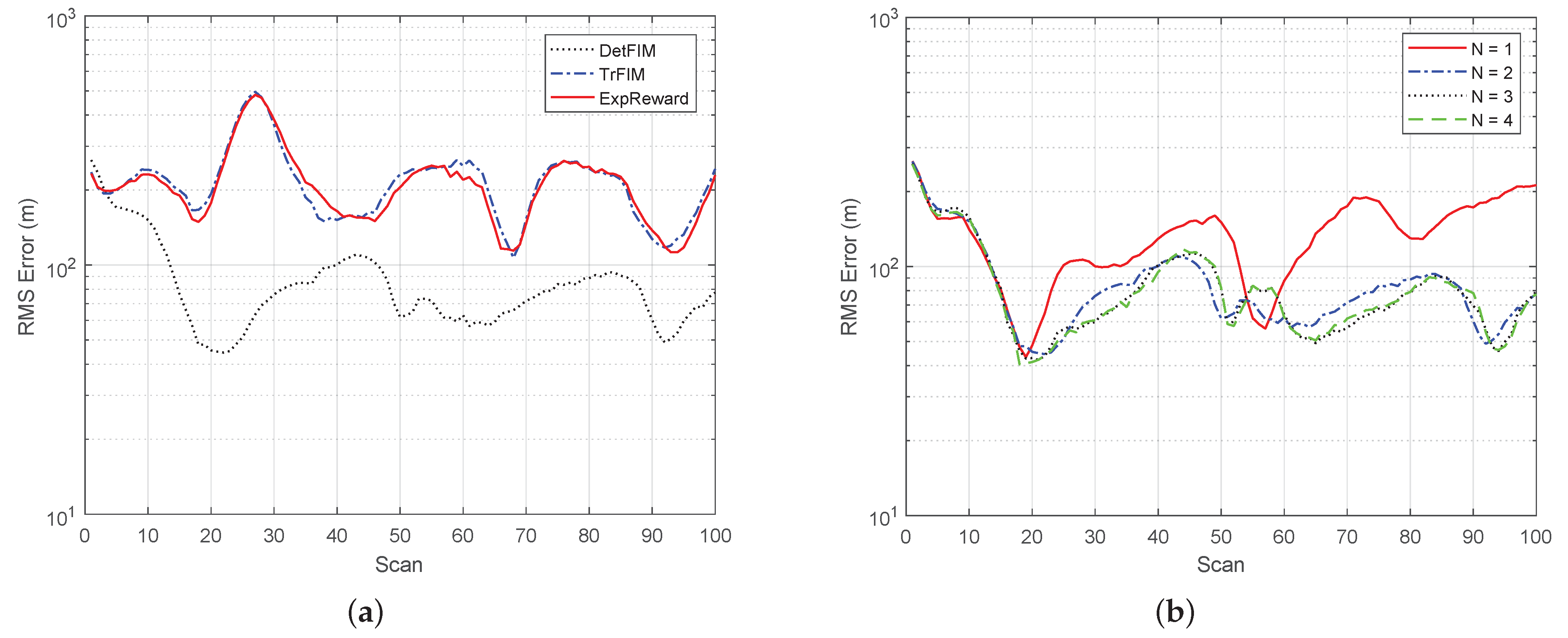
The statistical results averaged over 100 Monte Carlo runs for each case are shown in
Figure 7, where the root-mean-squared position error comparison of the tracker under different reward functions for
is presented in
Figure 8a, and the RMS errors under DetFIM for
are in
Figure 8b. In summary, the simulation results demonstrate that
the tracker yields a smaller error but significantly more computational overhead as
N increases. We observed that the computational complexity for
is roughly at a ratio of
when MaxH = 1000. Both computational overhead and RMS errors are bounded by MaxH, which is the maximum number of sensor trajectory hypotheses to be maintained. As shown in
Figure 8b, the RMS error performances for
are almost identical. This reflects the trade-off between error performance and computational load as the limited MaxH leads information loss due to the hypotheses pruning process:
the sensor scheduling under DetFIM yields a significantly small error, which is consistent with our analysis.
the RMS error under ExpReward is quite similar to that under TrFIM. The latter completely ignores the correlation between the two sensor states.
The major computational complexity of the simulation comes from the computation of N-Step ahead decision process when . For example, the average computational overhead per scan are 0.7 s when and 5.5 s for (on a machine with an Intel 2 Core i7-4600U CPU 2.10GHz processor (Intel: Mountain View, CA, USA)). The computational complexity difference between DetFIM, TrFIM and ExpReward are .


