1. Introduction
Sometimes drivers of vehicles leave the travel lane and encroach onto natural or artificial subjects on the roadside, causing a crash. These types of crashes account for a significant proportion of high-severity crashes [
1]. The installation of traffic barriers would be warranted if the severity of hitting these barriers would be less severe compared with hitting other roadside fixed objects. However even if this would be the case, the severity of colliding with these barriers would still persist. Previous studies mostly focused on analyzing the severity of traffic barrier crashes by analyzing traditional traffic barrier crash data, without aggregating those crashes across different barriers. In addition, previous studies mostly have ignored the frequency of those crashes in addition to the impacts of different crash severity types, e.g., fatality versus injury crashes. However, the crash frequency or crash severity alone could not account for the severity of crashes, especially if the objective of the assessment is to optimize the geometric characteristics of roadside barriers. One way to account for both crash frequency and crash severity is to consider property damage only (PDO) crashes as one single group and all other crashes against this PDO group based on their levels of severity, which would be weighted and converted into PDO crash equivalents. This measurement is known as the equivalent property damage only (EPDO) benchmark.
One of the biggest challenges of analyzing crash frequency along with crash severity is the distributional aspect of a model which cannot be modeled with distributions such as Poisson or gamma distributions. Despite a lack of studies employing EPDO, many studies have explored other aspects of traffic safety by considering only the frequency or severity of crashes. Nevertheless, it should be noted that the majority of those datasets which modeled crash counts were impacted by some forms of over- or under-dispersion resulting from the sparse nature of their crash counts [
2].
Some observations have an excess number of zeroes along with many small property damage only (PDO) crashes, which result in an overall mean that is close to zero. These types of distributions could not be modeled by using a traditional Poisson distribution, which considers the mean to be equal to the variance. However, this sparsity could be handled by using various methods incorporating various shape parameters, such as a negative binomial distribution.
Wyoming has one of the highest fatality rates in the United States [
3]. This is a result of many factors such as adverse weather conditions and mountainous areas with challenging roadways. Due to the presence of a large number of curves and mountainous areas, there is a significant number of traffic barriers in Wyoming. These barriers help in avoiding the severity of hitting other roadside fixed objects, but they still account for a number of severe crashes in the state.
The Wyoming Department of Transportation (WYDOT) funded a project to measure various aspects of more than 1 million linear feet of traffic barriers in the state. The objective of that project was to measure various aspects of the barriers’ geometric characteristics such as their heights and shoulder widths to better manage and enhance them. One of the main reasons for collecting the barrier geometric characteristics was that many of the barriers in the state are not within the recommended dimensions of barrier designs, and they should be enhanced. Having well-designed barriers is important because barrier crash severity would be further exacerbated if they are not well designed, resulting in possible override or underride barrier crashes.
Unfortunately, some of the barriers in the state are shorter or taller than the recommended heights, and some of those barriers have not been able to prevent any crashes. These barriers that did not experience any crashes have not been incorporated in the statistical analysis for traditional severity analysis because they have no response or explanatory predictors. However, since crashes are random events, there is a great likelihood that if those barriers experience any crash due to increased traffic, those crashes would be more severe compared with those involving well-designed barriers due to possible underride or override crashes. Thus, this study was conducted by considering the following points.
As there might be significant differences across different highway or interstate systems, this study only focused on interstate systems. While aggregating crash data across various barrier IDs, in order to keep the information of all predictors consistent, e.g., driver actions and environmental characteristics, the predictors were incorporated into the analysis by taking the average of those characteristics across different barriers. In addition, to account for both crash severity and frequency, both of these factors were incorporated in the model by using EPDO as a response. One of the challenges for the traffic barriers in Wyoming is testing the barriers that have not experienced any crashes. Due to the fact that crashes are random in nature, barriers that are not within recommended heights and did not experience any crashes were also incorporated in the dataset for analysis as well.
1.1. Problem Statement
Previous studies focus on various statistical methods based on intuition behind the distribution-based types of datasets, and are based on various goodness of fits. Although those studies implemented the correct statistical methods, the comprehensive investigations regarding implementing models were missing. For instance, the consequences of applying incorrect distributions on model parameter estimates are not entirely investigated. How would model parameters vary in the case of implementing the wrong distribution? Is there a lack of model strength that would result in failure of the correct estimation of model parameters? That is especially important when the objective is to implement the identified results for optimization purposes. In addition, the consequences of implementing an incorrect distribution have not been visualized extensively.
In this study, we conduct a comprehensive comparison on the performance of competing models to answer some of the questions above. Rootograms were used to highlight over- or under-fitting aspects for models with different values of EPDO for finalist models. Those models were compared not just in terms of goodness of fit but also in terms of model parameter estimates, along with other measures.
1.2. Literature Review
When analyzing crash frequency alone or combining that aspect with the severity of crashes, e.g., EPDO, various approaches have been employed to address the sparse nature of the data response. The following paragraph highlights some of the methodological approaches that have been followed to tackle the sparse nature and the presence of excess zeros in the dataset response.
The negative binomial model was used for modeling EPDO crashes in South Korea [
4]. One of the reasons for justifying the use of EPDO was to diminish the errors introduced by underreporting less severe crashes. Another study was conducted to examine the highway-rail grade crossing crash frequency model, which is characterized by under-dispersion [
5]. Different models such as the Conway–Maxwell–Poisson, hurdle Poisson, and zero-inflated models were considered and compared based on various criteria such as Alkaile Information Criterion (AIC). Readers can refer to the literature review for more information about Conway–Maxwell–Poisson [
6], hurdle Poisson [
7], and zero-inflated models [
8].
The EPDO crash rate was modeled using various hurdle regression frameworks to accommodate the excess number of zeros in the dataset [
9]. For the second layer of this model, crash counts greater than 0 and different distributions such as lognormal, gamma, and normal distributions were considered and compared. The results indicated that the lognormal hurdle model outperformed the other models.
The distribution of traffic crash rates were evaluated with various distributions such as lognormal hurdle and Tobit. Kolmogrov–Smirnov tests, kernel density, and quantile–quantile (Q-Q) plots were used to identify an appropriate distribution [
10]. The results show that lognormal hurdle can best fit a mixed and right-skewed crash rate.
The quantile regression model is another method applied in the literature review to model EPDO and identify crash blackspots [
11]; quantile regression used as crash data was highly skewed by the preponderance of zeros.
Despite efforts to model EPDO, little work has been made to model EPDO by the application of hurdle models with various distributional count models and to compare those results with other two-component models, e.g., zero inflated, and single-component model, e.g., Poisson model. Additionally, no studies have used EPDO for traffic barrier crashes by incorporating barriers that did not satisfy the recommended heights and barriers that have not experienced any historical crashes. The goodness of fit of various models was evaluated by measures such as Alkaile Information Criterion (AIC), and rootogram plots.
2. Method
In this study, barriers with crashes and risky barriers which did not experience any crashes were included in this study as crashes are random in nature. Not experiencing a crash does not mean that a barrier is not risky. This is especially true in a state like Wyoming with very low traffic. Although many of these barriers pose a high risk due to poor design, they have not experienced any crashes and there is a great chance that with an increase in traffic they would experience crashes. When these barriers experience crashes, the situation would be more severe if they are not within the recommended heights.
Different predictors were considered in the analysis to account for exposure resulting from differences across various barriers. For instance, variables such as barrier length and traffic were incorporated in the analysis.
Some of the issues with the crash data, especially EPDO, are over-dispersion or under-dispersion. Over-dispersion occurs when sample variance is higher the mean, while the reverse is true for under dispersion. These challenges could be a source of errors by specifying a model with the wrong distribution, which results in potential errors and biased coefficient estimates. When the data is over-dispersed, some changes in the model parameters could be applied to account for that over dispersion, e.g., application of a negative binomial model [
12].
In general, the count model can be modeled by the generalized linear model (GLM). For Poisson, the variance would be set as identical to the mean and the dispersion parameter is fixed at
. In other words, for the Poisson model, the variance is restricted to the mean as shown below:
Poisson model has a linear form as:
where
βs are the estimated regression coefficients, and x
s are different explanatory variables.
Quasi-Poisson model is another method of GLM that can handle over-dispersion. For this model, compared with a standard Poisson, would be unrestricted on the left. In other words,, instead of being fixed, would be calculated from the data.
Negative binomial is a type of Poisson model, Poisson-gamma mixture model, that can be used to relax the constraint of equality between the mean and variance. The negative binomial can be written as follows:
where the Poisson parameter
follows a gamma probability distribution, Exp(
) is a gamma-distributed error term, and other parameters were defined earlier.
As discussed, a negative binomial can be used as gamma mixture of Poisson distribution. This model has
where variance differs with the Equation (4):
where
is a shape parameter, and
is the mean.
In addition to over-dispersion, many count data exhibit an excess number of zero observations, which might not be addressed by GLM models [
13]. The zero-inflated model, for example, is a method that can account for over-dispersion and the presence of excess zeros. This model allows zeros to come from both at-risk (sample zeros), and not-at-risk populations (structural zeros), while the hurdle model only allows zeros to come from at-risk populations [
14]. For those models, sample zeros would be calculated by a binary logistic model, while structural zeros would be estimated by the count part of the model, e.g., negative binomial or Poisson model.
By design, if the interest is to design a model that incorporates only sample zeros and at-risk samples, then the hurdle model is preferred. Although it has been discussed that zero-inflated is preferred in many count datasets due to its improved statistical fit, it has been argued that the inherent dual state process underlining the development of this model is inconsistent with crash data [
15].
Another issue with the zero-inflated model for modeling crash data is that this model assumes the extra zeros come from two states: a true-zero state, where the roadway locations are inherently safe meaning that no crash would occur on those roadway locations at any time, and non-zero state where only no crashes occurred in the observation periods [
16]. It should be noted that it is unrealistic to consider any road segment as safe at all times, which makes the zero-inflated model unsuitable for crash counts with an excess number of zeros. On the other hand, the hurdle model addresses the assumption of the zero-inflated model by assuming that roadway segments with zeros are only safe over the study period and not at all times [
9].
The hurdle model, as a substitute for the zero-inflated model, is a model that could be used to account for excess numbers of zeros and over-dispersion. There are two layers for these models including a truncated count and values greater than zero, which could be accounted for by Poisson, geometric or negative binomial distributions. On the other hand, a hurdle component models zero count by using binary logistic regression to evaluate a change from zero crash to crash areas.
For the hurdle model, a probability of mass function (PMF) could be written as [
7]:
where
π is the probability that the response
= 0 and 1−
π is the probability that
.
For the Poisson process as a starting point of count data, the above formula for zero-truncated Poisson has the PMF as follows:
where
is an expected number of 0, 1, 2, …,
y and
is the predicted EPDO for every barrier.
Thus, from Equations (1) and (2), the unconditional probability mass function for
Y is:
If
is modeled by log-log and
is modeled by log link, with some algebra for the hurdle model and Poisson count, we would have:
and
and after some algebra the log likelihood could be written as:
It can be seen from the Equation (10) that the log likelihood of zero and not zero could be written as the sum of the two. In other words, this model estimates the probability of two models: one for zero values and one for non-zero values.
In the results section, the hurdle and zero-inflated models are two-layer models. The first layer for the hurdle model is a logistic model governing observations with zero and greater than zero values. The second part is a zero-truncated count model governing the outcomes with positive counts. This model is flexible not only to account for excess zeros but for under- or over-dispersion distribution based on the defined distribution for the second layer.
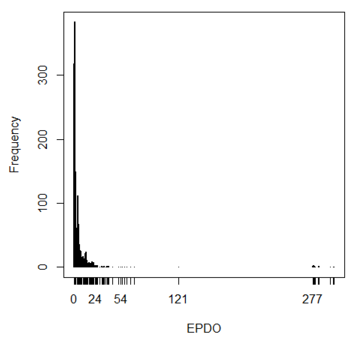
Figure 1 is presented to highlight the sparse nature of barrier EPDO crashes. As can be seen from this figure, EPDO is highly skewed to the left with most observations being less than 50, EPDO is mainly 1, and there are few large observations. The description of this response in
Table 1 provides more information.
In this study, all the discussed methodologies were implemented to highlight the impact of considering inappropriate distributions. Although it has been discussed that using the wrong distribution for data analysis would result in biased and erroneous results, this study delves into the possible erroneous outcomes by estimating all the coefficients for different distributions and evaluating them based on various goodness-of-fit measures.
3. Data
The crash data were obtained from the Critical Analysis Reporting Environment (CARE) package, which provides comprehensive information regarding various aspects of variables such as vehicles and drivers being involved in a crash. This dataset does not include information related to the roadside geometric characteristic or geometric features of traffic barriers. Thus, this information was obtained and aggregated to the traffic barrier dataset from another source: the information related to 1.3 million feet of traffic barriers was collected from a field survey performed by a WYDOT contractor. The collected information includes various information such as shoulder width, barrier length, height, and offset.
Only single vehicle crashes were considered in this study. This is because the severity of multiple vehicle crashes might be due to unseen confounding factors that the included variables could not account for. In addition, due to significant differences across a variety of roadway classifications such as interstate and highway systems, only interstate crashes were considered in this study. The data set includes barriers crashes between 2007 and 2017. These crashes were matched with barriers based on their mile posts and highway route IDs.
This resulted in identification of 1069 barriers along 139 miles of roadway, which experienced at least one crash of any severity level during the time period. A significant portion of barriers in the Wyoming interstate system did not experience any crashes. In addition, some of these barriers have heights below or above the recommended heights based on barrier design guidelines. Having higher barriers could result in underride crashes while the reverse could result in override crashes. These types of crashes are historically more severe that other barrier crashes.
The critical values for override and underride crashes are considered in this study as below 27 inches and above 35 inches, respectively [
17]. It should be mentioned that the higher height limits do not apply to concrete barriers since underride in not plausible for that barrier type. Almost all concrete barriers experienced some form of crash as these barriers are mainly installed as median barriers, which exposed them to a high number of crashes.
Barriers with no crashes were incorporated based on the randomness of crashes. There is a high risk of severe crashes for these barriers due to under- or over-ride crashes. Therefore, these barriers were identified and incorporated in the final model on the interstate system. This resulted in identification of a total of 235 barriers along 20 miles of roadway that did not experience any crashes but were below or above the recommended heights.
In summary, the whole dataset used in this study incorporated 1388 traffic barriers including barriers with and without crashes. While the whole dataset included barriers’ geometric characteristics and traffic volumes, barriers with crashes have additional information such as driver action characteristics. Since some barriers experienced more than one crash and each crash has various driver, roadway, and weather characteristics, the averages of those values were included in the dataset. In Wyoming, the economic costs for various crashes could be calculated as:
Based on the above Equation (11), a fatal crash, for instance, is equivalent to 277 PDO crashes.
Table 1 presents the descriptive statistics of the included variables found to be important in the statistical section for both barriers with and without crashes. As discussed earlier, as a barrier might experience more than a single crash with various driver and roadway characteristics, the averages of those variables were incorporated in the final dataset. For instance, as can be seen from
Table 1, the mean for restraint constraint is 0.11. That means that the majority of drivers hitting a barrier had some form of restraint at the time of crashes (restraint constraint with safety in use was set as 0).
Different predictors such as the Average Annual Daily Traffic (AADT) and barrier length were incorporated into the analysis to account for exposure effects. Barrier types were incorporated into the study to account for differences across various barrier types. For these predictors, only frequency is presented in
Table 1. Furthermore, as seen in
Table 1, barriers with no crashes suffer from a higher variation, in terms of variance, compared to barriers with crashes. They also present a lower barrier height compared to barriers with crashes, indicating that those barriers were mostly below the recommended height of 27 inches.
Regarding the shoulder width variable, while categorical aspects of shoulder width were considered for the first layer of a hurdle model, a continuous feature of this predictor was found to be important for the second layer of this model. There are a total of 257 miles of traffic barriers in the interstate system in Wyoming. Among this number there was a distance of about 10 miles of barriers that did not receive any crashes during the 10 year period. That number is added to 138 miles of barriers that did receive some form of crash. There are also about 109 miles of newly built barriers following the acceptable height where the heights were not measured. Due to lack of availability of height, and due to the fact that those barriers have already been optimized due to new installation, these barriers were removed from the analysis.
4. Performance Evaluations of Models
To evaluate the performance of models’ goodness of fits, the literature review regularly checks the residuals, or deviation of observation yi from the corresponding predicted means. This approach has been used to ensure that after transforming the dataset, e.g., response, the model residuals follow a normal distribution. This can be achieved by checking quantile–quantile (Q-Q) plots. This is a scatterplot created by plotting two sets of quantiles against one another to check if both sets come from the same distribution.
Various measures such as the Akaike Information Criterion (AIC) were used in this study for a comparison across various included models. The AIC was used to compare various incorporated models. This measure follows .
Where k is the number of model parameters including the intercept, and likelihood is a measure of model fit. The benefit of this measure over others, such as log likelihood, is that this measure includes a penalty for including more predictors, preventing an over-fitted model from being highlighted to have a better fit.
Rootograms have been designed for diagnosing and addressing issues such as over dispersion and an excess number of zeros in the data [
2], being extended from Tukey’s work in the literature review [
18]. This is an improved approach to the assessment of a count model such as Q-Q plot. There are a few important observations that should be taken into account while using this figure:
Based on the identified model, expected counts are shown by a red line.
Real/observed counts are shown as bars.
X-axis represents counts.
Y-axis represents square root of expected/observed counts.
The first line observed in this figure is related to the height of the observation with zero value (EPDO = 0).
In this study, the use of rootograms plots were implemented after identification of a best model distribution to make sure the finalist models follow the right distribution.
5. Results
The following section will detail the results shown below. The model comparisons present a comparison between models with different distributions. The second section will discuss the results of the finalist models, hurdle models with two different distributions based on rootograms, and the last section will describe the results of the best-fit model.
5.1. Model Comparisons
Table 2 is presented to make a comparison between different fitted models based on count data regressions. The response was EPDO and similar predictors were incorporated in the models. However, it should be noted that while all included models incorporated similar predictors, zero-augmented models, model zero observation and crash barriers separately while GLM accounted for both layers in one model. While log likelihood is not a fair comparison across various models due to the different number of parameters for each model, AIC measures could penalize incorporating various predictors for each model. Thus this measure could be used for the purpose of comparison across different models.
It is of interest not only to find the best-fit model but to make a comparison across parameters’ estimations with various distributions. From
Table 2, three GLM models and two zero-augmented models were considered. It should be noted that both zero-augmented models used logit link function for their first layers. It can be seen from Poisson and quasi-Poisson that the estimates are almost identical. However, while almost all the included variables are important at 0.05
p-value significance for the Poisson model, many estimations are significant not for quasi-Poisson models. This is due to the fact that the scale parameter is fixed as 1 for Poisson while this value is computed for quasi-Poisson. Not accounting for over-dispersion, even if that model results in very similar output coefficient estimates, it would result in unreasonable inference/interpretation.
Moving to GLM with the family of negative binomial, it can be seen that while there are some similarities between negative binomial and Poisson, and also quasi-Poisson models. It can be observed that while there are similar signs for various driver action variables between negative binomial results and the other GLM models, there are significant differences for barriers and roadway characteristic predictors, shoulder width, barrier height, and the correspondent interaction terms. While quasi-Poisson is not associated with a fitted likelihood, the negative binomial improved the fit dramatically compared to the Poisson distribution (AICNB = 6955 versus AICpoisson = 29,630). In summary, even considering a different family of GLM results in complete variations across some predictors in terms of signs and magnitudes.
For zero-augmented models, two components need to be clarified for the models. One component for values greater than zero and another component for zero observations, which are often defined by the binary logistic regression model. For the non-zero distribution, logit link function was considered for both the zero-inflated and hurdle models. The Poisson distribution is considered for the non-zero hurdle model as well, which will be evaluated in the next section.
For the most part, the estimates for both zero-augmented models are very close with similar signs for all significant predictors in the non-zero layer. The inverted signs of the zero-inflated model are expected. As for the hurdle model, the zero hurdle component describes the likelihood of observing a crash while the zero-inflated component predicts the probability of observing a zero count. In summary, both zero-augmented models have two layers: the first layers controls whether a vehicle hits a barrier or not and the second component controls how many times and with what crash severity level a vehicle would hit a barrier.
In summary, a significant improvement was observed by implementing the GLM with negative binomial distribution compared with the GLM Poisson model. These results were expected as Poisson distribution does not account for over-dispersion. Although a slight improvement was observed from the negative binomial to the zero-inflated model, the improvement was greater when compared to the hurdle model.
5.2. Comparison Between Hurdle Models, Truncated Count Component, with Different Distributions
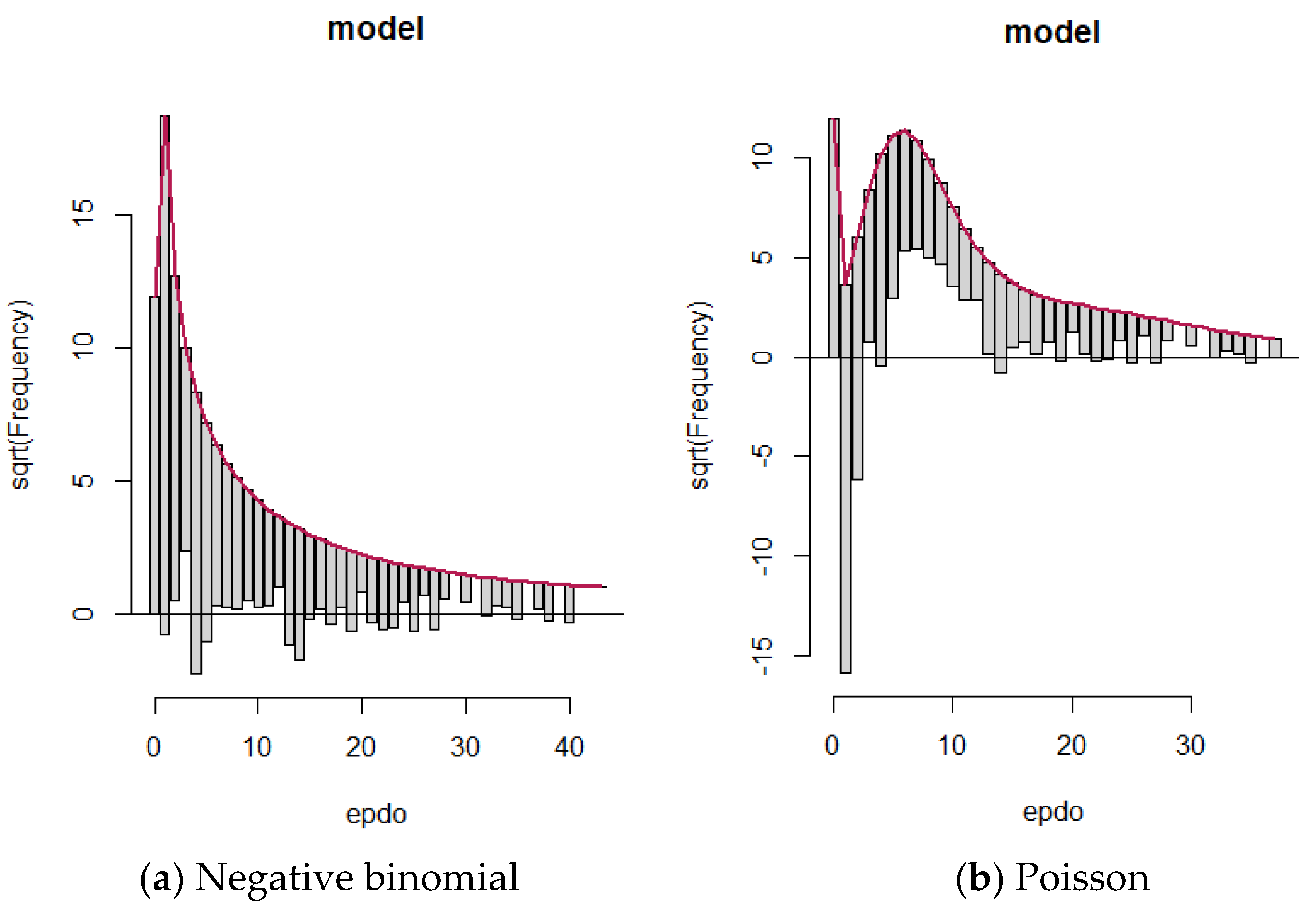
Based on the discussion in the paragraph above, hurdle models were identified as the best-fit model across the included competing models. However, this model is a two-component model with a truncated count component. The truncated count component, which is used for positive count, can take different distributions. This section considers only Poisson and negative binomial distributions as these two distributions are more likely to be able to fit non-zero portions of this model. It is clear that Poisson is not suitable for our dataset, but for comparison purposes and to visualize how they fit the observations, these two models are compared to see how they fit the observations. The rootogram was chosen for comparison across these models to make sure the right distribution is chosen for a final model.
The rootograms allow us to visualize if the model is over- or under-fitting for different values of EPDO as response. For rootograms, only the values less than EPDO = 50 were considered to improve readability. These values accounted for more than 98% of all the included observations.
As discussed in the method section, the first line observed in these figures is related to the height of observations with zero value (EPDO = 0). As can be seen from rootograms,
Figure 2a,b, the hurdle components of the models that model zero counts fit zero values quite well. It is expected for these models to fit zero count perfectly by design. However, when EPDO is equal to 2 or 3, while a dramatic under-fitting can be observed for Poisson distribution, the negative binomial layer could fit those values quite well.
In other words, for the Poisson model, the substantial amount of over-dispersion in the data could not be accounted for by this model. It should be noted that the EPDO values equal to 2 or 3 account for 50% of all the EPDO > 0. From EPDO = 6 onward to EPDO = 14, the Poisson model basically does not predict any count because it is over fitting, while the negative binomial distribution, for the most part, fits the data fine. In summary, as can be seen from
Figure 2, the negative binomial model fits the model quite well while the Poisson model suffers from over-dispersion/under-dispersion issues.
5.3. Hurdle Model Results
As the hurdle model with negative binomial was identified as the best identified model, this section briefly discusses the results obtained from
Table 2. The results of the hurdle model include two components. The first layer includes the impact of various predictors on the frequency of EPDO. First, it was found that the impact of barrier height and shoulder width on EPDO should not be considered separately, but rather should be considered as interactive terms that impact crash severity. Non-compliance with the speed limit and being unrestrained were two of the factors that were found to increase the risk of EPDO crashes, with the impact of the restraint condition being much higher than the impact of the other variable, 2.482 versus 0.89.
Moving to the next layer of the hurdle model, as a crash did not occur in this section, only predictors related to the road and barrier geometric characteristics were considered. Barrier length and traffic are two factors that were considered to account for exposure. The coefficient estimates with positive signs indicated the contributory impacts of those predictors in predicting a crash compared with no crash. For instance, as can be expected, higher barrier length and higher traffic (AADT) increase the odds of having a crash. Additionally, the interaction between shoulder width and barrier height were found to impact the odds of having a crash. However, the differences across magnitudes and signs between these two layers should be noted.
6. Summary and Conclusions
The installation of traffic barriers would be warranted if they could reduce the severity of fixed object crashes. However, barrier crash severity will still exist when hitting a barrier. Actually, traffic barrier crashes are a major social and economic concern due to their high severe crash rate for policy makers, especially in a mountainous area like Wyoming with significant under/over standard barriers heights needing immediate attention.
Studies in the literature review only focused on the severity of barrier crashes. However, crashes are random and not experiencing a crash does not indicate that a specific barrier is not hazardous. The condition would be more critical if those barriers were below standard design, and also if they did not experience a crash. In addition to barriers with crashes, this study incorporated barriers with no crashes that were not designed based on the recommended height, posing a danger of underride or override crashes.
To account for both severity and the frequency of crashes, EPDO was used as a measure that could account for both aspects of crashes. The distribution of responses shows a substantial amount of over-dispersion that cannot be accounted for by a Poisson model. In addition, the number of zeros were so large that just correcting for over-dispersion through the negative binomial model cannot address the issue. Thus, in order to identify the right distribution, various models were considered and the best-fit model was identified based on various measures.
AIC measure was used for a decision across various model distributions. A comparison was used not only between various goodness-of-fit measures across the included models, but also between the sign and magnitude of various coefficient estimates. The results indicated that considering the wrong distribution would not only result in a biased estimation of the coefficients for some predictors, but the signs of some critical predictors such as barrier height would be reversed. This would result in a tremendous waste of public funds if it would have not been addressed properly.
The comparison results based on various measures work in the favor of the hurdle model. Rootograms was used to make the decision of the truncated hurdle model by considering negative binomial and Poisson distributions. Although the negative binomial distribution seems to be suitable for the sparse nature of the dataset, the rootograms visualize how various models would fit the observations. These measures highlighted that the negative binomial distribution for the first component of the hurdle model could fit the data quite well. It is recommended for future studies to give attention to a model distribution assessment while considering crash frequency or EPDO. An optimization technique would be considered for barrier optimization in the Wyoming interstate system.


