A Recursive Generative Adversarial Denoising Learning Method for Acoustic-Based Gear Fault Diagnosis Under Non-Stationary Noise Interference

Abstract

Acoustic-based diagnosis (ABD) technology demonstrates promising application prospects for rotating machinery such as gears. However, non-stationary background noise may obscure or distort the target acoustic signal, potentially resulting in misdiagnosis or inadequate diagnosis in practical application. Therefore, preserving the inherent periodicity and sparsity features of mechanical sound signals from non-stationary background noise constitutes a critical challenge to facilitating the effective application of ABD in practical industrial environments. To address the shortcoming, this paper proposes an ABD method based on Recursive Generative Adversarial Denoising (RGAD). Specifically, a Global Window-aware Attention Module (GWAM)-based generator is first designed to reconstruct periodic structural features of gear rotational acoustic signals by adaptively representing non-stationary noise components and recursively capturing global dependencies in the time–frequency domain. Subsequently, a generative adversarial mechanism is established through developing a recursive discriminative architecture, which enables the model to effectively alleviate the vanishing gradients during adversarial learning and recover the texture details of gear acoustic features in a coarse-to-fine manner through progressive guidance. Finally, combined with a fault diagnosis network (FDN), a complete RGAD-based ABD framework is constructed. Experimental results demonstrate that the proposed method effectively suppresses noise components while simultaneously reconstructing the periodic characteristics and fine texture details of gear rotational acoustic signals, thereby significantly improving the accuracy and reliability for gear acoustic diagnosis in real industrial scenarios.

1. Introduction

Gears are an essential component of modern rotating machinery and are widely used in various fields such as wind power generation, aerospace, and transportation. Gear fault diagnosis has always been a challenging and highly researched topic, as the operating condition of gears directly affects the performance of the equipment and the personal safety of workers [1,2]. Although vibration-based gear fault diagnosis methods have been commonly used and have achieved good results, the installation of vibration sensors is often limited by working conditions and the complex structure of the equipment to be diagnosed. Moreover, vibration signals are difficult to measure in certain special environments [3].

In recent years, non-contact acoustic-based diagnosis (ABD) methods have attracted increasing attention due to their ability to complement traditional vibration-based techniques. Early studies by Rezaei et al. [4] investigated the effectiveness of ABD for bearing fault detection under varying speeds and load conditions. Peng et al. [5] proposed an acoustic signal-based anomaly detection framework for industrial machinery, enhancing detection accuracy through time–frequency feature perception, further confirming the feasibility and stability of acoustic signals for diagnosis. In the field of rotating machinery, Scanlon and Zhang et al. [6,7] applied non-contact microphone sensors for health monitoring of rotating machinery. Hassan et al. [8] employed a physics-informed deep learning approach to develop an acoustic-based engine fault diagnosis method. Furthermore, in the field of gear fault detection, Hou et al. [9] developed acoustic fault mode detection methods based on near-field acoustic holography, successfully capturing the sound field characteristics of gears in complex structures. Meanwhile, Yao et al. [10,11] proposed a series of air-coupled acoustic diagnostic approaches integrating deep learning and attention mechanisms, which improved gear fault recognition accuracy and real-time performance through automatic feature extraction. Glowacz et al. [12,13,14] introduced innovative acoustic features and applied ABD to the fault diagnosis of various devices, including induction motors, electric impact drills, coffee grinders, and commutator motors, demonstrating strong generalization capabilities. In addition, Ebrahimkhanlou et al. [15] integrated deep learning with acoustic technology and applied it to complex plate-like structures for acoustic emission source localization and characterization. Despite the promising performance of these ABD methods in rotating machinery diagnostics, most studies have been conducted under noise-free or ideal laboratory conditions, with insufficient consideration of background noise. This creates a performance gap between experimental results and practical applications. In real-world industrial scenarios, intense and highly non-stationary background noise presents a critical challenge for ABD tasks—originating from machine collisions, abnormal bearing wear, and complex disturbances caused by load fluctuations in machining systems. These interferences severely degrade the separability of acoustic features and remain a major obstacle to the practical deployment of ABD methods [3]. However, to our knowledge, few studies have so far been reported on separating acoustic characteristics from non-stationary background noise for a precise diagnosis. But similar acoustic signal separation and enhancement methods have been widely studied in the field of speech processing, which can provide valuable insights for noise suppression in ABD applications.

In traditional speech processing, non-stationary noise suppression methods include spectral subtraction [16], filtering-based denoising [17], and minimum mean square error (MMSE) estimation [18]. Among these, filtering methods are widely applied. Haykin et al. [19] first proposed Least Mean Square (LMS), a traditional adaptive filtering algorithm based on Wiener filters. Subsequently, Martinek et al. [20] proposed Recursive Least Squares (RLS), a representative adaptive filtering algorithm, based on Kalman filtering theory [21]. However, the aforementioned methods rely on statistical properties between speech and noise and cannot guarantee signal reconstruction quality in highly non-stationary environments due to often introducing artifacts such as “musical noise”. To overcome this limitation, deep learning-based methods have been further developed for high-quality speech reconstruction in non-stationary environments, which are typically divided into masking-based and mapping-based approaches. Masking-based methods learn ideal time–frequency masks, such as ideal binary mask (IBM) [22] and ideal ratio mask (IRM) [23], but their performance drops significantly when faced with unseen noise. In contrast, mapping-based methods directly predict clean speech using deep neural networks [24], and they employ strategies like noise-aware training [25] and batch normalization to improve generalization. Although more robust to unknown noise, mapping methods often offer slightly lower fine-grained details than mask-based approaches [23]. Considering the issues of fine-grained speech reconstruction in unseen noise, the Generative Adversarial Network (GAN) is involved in the speech processing task for texture detail enhancement. Pascual et al. [26] first investigated generative architectures, called SEGAN, for speech enhancement at the waveform level. Pandey et al. [27] comprehensively verified the superiority of adversarial training compared to regularization-based training for noise enhancement. Fu et al. [28] proposed MetricGAN, which improves speech enhancement performance by replacing traditional adversarial loss with surrogate functions to enhance speech intelligibility and quality. MetricGAN+ [29] further optimizes the training strategies based on this foundation, demonstrating better generalization capabilities across various speech enhancement tasks. Additionally, Wang et al. [30] proposed T-F Masking, which employs a generative adversarial mechanism to construct masks in the time–frequency domain, effectively suppressing noise components under non-stationary conditions. Although the existing generative architectures in the field of speech processing provide sufficient reference for generative-based non-stationary noise suppression strategies in ABD tasks, the speech generative-based framework may not be suitable for acoustic-based gear fault diagnosis due to the unique periodicity and sparsity characteristics of gear operating sounds.

To address the aforementioned challenges, a Recursive Generative Adversarial Denoising learning method (RGAD) is explored for acoustic-based gear fault diagnosis in real industrial noise environments. Inspired by the Swin Transformer for capturing global dependency in a sequence signal, the Global Window-aware Attention module (GWAM) is first introduced to restore the periodic structure of the gear acoustic signal on the time–frequency spectrum. Unlike the original design of the Window-based Multi-Head Self-Attention (W-MSA) that shifts at the patch level, the GWAM focuses on global patches of the spectrum for periodic feature reconstruction from non-stationary background noise. After repeatedly embedding the GWAM unit to form the generator, a recursive discriminative architecture is further developed to construct a basic adversarial mechanism, where discriminators with different capabilities are placed in different parts of the generator to interact with equivalent GWAM units for playing max-min games. This design effectively avoids vanishing gradients during the adversarial process and guides the generator to gradually eliminate noise components and progressively restore the texture details of the target clean spectrum in a coarse-to-fine manner. Finally, the RGAD is integrated with a well-trained fault classification module to construct a Recursive Generative Adversarial Denoising diagnosis framework for acoustic-based gear fault diagnosis in real industrial noise scenarios. Experimental results demonstrate the superiority of the proposed RGAD-based ABD framework in both noise suppression performance and diagnosis accuracy compared to conventional approaches.

The main contributions delivered in this work are summarized as follows:

• A novel GWAM-based generator is first proposed to capture the periodic structure characteristics of gear acoustic signals under noise interference by adaptively representing non-stationary noise components and recursively modeling the global dependence of time–frequency features.
• A new adversarial mechanism is further developed by constructing a recursive discriminative architecture, which enables the model to effectively avoid the vanishing gradient problem and significantly refine the detail reconstruction quality of acoustic features from the noise condition.
• Building upon the above modules, a complete RGAD-based ABD framework is constructed to detect gear fault patterns in non-stationary noise conditions, which demonstrates the effectiveness of the proposed ABD framework in real industrial scenarios.

2. Background

2.1. Swin Transformer

The Transformer architecture was originally proposed by Vaswani et al. [31], featuring a Multi-Head Self-Attention mechanism as its core component. It has achieved remarkable success in both natural language processing and computer vision tasks. The traditional Transformer block consists of Layer Normalization (LN), Multi-Head Self-Attention (MSA), and a Multi-Layer Perceptron (MLP), where LN is applied before each MSA and MLP module. These core components are integrated via residual connections, which can be expressed as

$$\begin{array}{cc}\hfill {\widehat{z}}^l& =\mathrm{MSA}\left(\mathrm{LN}\left(z^{(l-1)}\right)\right)+z^{(l-1)},\hfill \\ \hfill z^l& =\mathrm{MLP}\left(\mathrm{LN}\left({\widehat{z}}^l\right)\right)+{\widehat{z}}^l,\hfill \end{array}$$

(1)

where $z^l$ represents the output of the $l^{\mathrm{th}}$ Transformer block. ${\widehat{z}}^l$ denotes the intermediate features after passing through the MSA module. The MSA mechanism captures long-range dependencies in input sequences by computing attention weights between queries (Q), keys (K), and values (V). Its core computation can be represented as

$$\begin{array}{c}\hfill Q=z^l{W}_Q,K=z^l{W}_K,V=z^l{W}_V,\\ \hfill \mathrm{MSA}\left(z^l\right)=\mathrm{Softmax}\left({\displaystyle \frac{Q{K}^T}{\sqrt{d}}}\right)V.\end{array}$$

(2)

The MSA is computed by first obtaining the dot product between the query matrix (Q) and the transposed key matrix ($K^T$), scaled by the reciprocal square root of the feature dimension $\sqrt{d}$. This scaled attention score matrix is then normalized through the Softmax activation function along the sequence dimension to generate attention weights, which subsequently interact with the value matrix (V) via matrix multiplication to produce the context-aware output representation.

In the conventional Transformer, input tokens need to be computed based on its relationships to all other tokens through the standard MSA mechanism, where the computational complexity is quadratic to the number of tokens. This makes it impractical for high-resolution inputs and resource-constrained applications. To address this issue, Liu et al. [32] proposed the Shifted Window Transformer (Swin Transformer), which adopts a “window-MSA + shifted window-MSA” strategy to significantly reduce computational complexity while preserving modeling capability. The formulation for W-MSA can be represented as follows:

$$\begin{array}{c}\hfill \mathrm{W}-\mathrm{MSA}\left(z^l\right)=\mathrm{Softmax}\left({\displaystyle \frac{Q{K}^T}{\sqrt{d}}}+B\right)V,\end{array}$$

(3)

where B is the relative positional bias term.

To alleviate the interaction limitation between windows, SW-MSA is introduced following the W-MSA structure for cross-window interaction without additional computation. Different from the W-MSA structure, the SW-MSA employs a cyclic-shifting mechanism to aggregate non-adjacent sub-windows from feature maps for promoting information interaction. With this shifted window partitioning mechanism, the definition of the SW-MSA can be written as

$$\begin{array}{c}\hfill \mathrm{SW}-\mathrm{MSA}\left(z^l\right)=\mathrm{SoftMax}\left({\displaystyle \frac{Q{K}^T}{\sqrt{d}}}+B+M\right)V,\end{array}$$

(4)

where M is a predefined binary mask matrix. It enforces the attention computation to be performed only within specific sub-windows after the shift operation by setting the attention scores between non-adjacent patches to negative infinity.

2.2. Generative Adversarial Network

Generative Adversarial Networks (GANs) were first proposed by Goodfellow et al. in 2014 [33]. The core idea of the GAN is to use two networks, a generator G and a discriminator D, which engage in adversarial training to model the distribution of data by generating realistic samples from random noise:

$$\begin{array}{cc}\hfill & {\mathcal{L}}_{GAN\left(G\right)}={\mathbb{E}}_{z\sim p_z}[log(1-D\left(G\left(z\right)\right))],\hfill \\ \hfill & {\mathcal{L}}_{GAN\left(D\right)}={\mathbb{E}}_{x\sim p_{data}}[logD\left(x\right)]-{\mathbb{E}}_{z\sim p_z}[log(1-D\left(G\left(z\right)\right))],\hfill \end{array}$$

(5)

where x∼$p_{data}$ represents real samples from the data distribution and z∼$p_z$ is the noise vector.

The discriminator attempts to maximize the ability to distinguish between real and fake samples, while the generator tries to generate fake data that fools the discriminator. In recent years, the GAN has shown significant potential in tasks such as image super-resolution and speech enhancement, where it demonstrates strong generative power for learning complex, high-dimensional features [26]. Compared to traditional denoising methods, the GAN is more robust to non-stationary noise and is capable of learning intricate noise patterns. Moreover, GANs can learn more complex features and background noise patterns, offering stronger modeling capabilities for highly dynamic and non-stationary acoustic signals. The GAN’s ability to model and separate these signals makes it a promising approach for tasks that involve complex interference or environmental noise [34].

Considering that the classical method is potentially affected by vanishing gradients due to the sigmoid cross-entropy loss used for training, the least-squares GAN (LSGAN) approach substitutes the cross-entropy loss by the least-squares function with binary coding. With this in mind, the formulation in Equation (5) changes to

$$\begin{array}{cc}\hfill & {\mathcal{L}}_{LSGAN\left(G\right)}={\displaystyle \frac{1}{2}}{\mathbb{E}}_{z\sim p_z}\left[{(D\left(G\left(z\right)\right)-\beta )}^2\right],\hfill \\ \hfill & {\mathcal{L}}_{LSGAN\left(D\right)}={\displaystyle \frac{1}{2}}{\mathbb{E}}_{x\sim p_{data}}\left[{(D\left(x\right)-\alpha )}^2\right]+{\displaystyle \frac{1}{2}}{\mathbb{E}}_{z\sim p_z}\left[{(D\left(G\left(z\right)\right)-\beta )}^2\right],\hfill \end{array}$$

(6)

where $\alpha =1$ and $\beta =0$ denote true labels and false labels.

3. Methodology

In this section, the GWAM, which is a core component of the generator responsible for the extraction of periodicity characteristics, is first introduced. Then, the proposed adversarial mechanism comprising a recursive discriminative architecture is further described. Subsequently, the overall architecture and optimization strategy of RGAD are elaborated sequentially. Finally, the complete RGAD-based ABD framework and corresponding diagnosis procedure are presented.

3.1. Global Window-Aware Attention Module

As the core component of the generator in the RGAD model, the designed Global Window-aware Attention Module (GWAM) consists mainly of Layer Normalization (LN), Window-based Multi-Head Self-Attention (W-MSA), residual connections, and a Multi-Layer Perceptron (MLP). It is responsible for capturing the periodic structural features of gear rotational acoustic signals under non-stationary noise by establishing long-range time–frequency (T-F) dependencies. The operational mechanism is illustrated in Figure 1. Let the original noisy time–frequency input signal be denoted as $x_n\in {\mathbb{R}}^{T\times F\times 1}$, where T and F represent the time frames and frequency bins, respectively. The input spectrum is partitioned into P patches of size $T^{\prime }\times F^{\prime }$ to form localized T-F representation $x_n^p\in {\mathbb{R}}^{{\displaystyle \frac{T}{T^{\prime }}}\ast {\displaystyle \frac{F}{F^{\prime }}}\times T^{\prime }{F}^{\prime }}$, where $P={\displaystyle \frac{T}{T^{\prime }}}\ast {\displaystyle \frac{F}{F^{\prime }}}$. After the $x_n^p$ are projected into the patch embedding space and normalized using LN, the patch embedding features are fed into the W-MSA module for exploring T-F dependencies on global patches. Specifically, $x_n^p$ is projected through three linear layers to obtain high-dimensional ($(3\ast T^{\prime }{F}^{\prime })$) query (Q), key (K), and value (V) matrices, which are computed by

$$\begin{array}{c}\hfill Q=x_n^p{W}_Q,\end{array}$$

(7)

$$\begin{array}{c}\hfill K=x_n^p{W}_K,\end{array}$$

(8)

$$\begin{array}{c}\hfill V=x_n^p{W}_V,\end{array}$$

(9)

where $W_Q$, $W_K$, $W_V$ are learnable parameter matrices of size $[T^{\prime }{F}^{\prime },3\times T^{\prime }\times F^{\prime }]$, and the dimensions of the output Q, K, V are $[P,3\ast T^{\prime }{F}^{\prime }]$. Next, we set the number of attention heads to h and perform attention splitting on Q, K, and V:

$$Q,K,V\stackrel{Split}{\to }{Q}_i,K_i,V_i\in {\mathbb{R}}^{h\times P\times {\displaystyle \frac{3\ast T^{\prime }{F}^{\prime }}{h}}},$$

(10)

where i denotes the i-th attention head. The global attention weight $H_i$ for a single attention head is computed as follows:

$$H_i=\mathrm{Attention}(Q_i,K_i,V_i)=\mathrm{Softmax}\left({\displaystyle \frac{Q_i{K}_i^T}{\sqrt{d}}}\right)V_i,$$

(11)

where ^T denotes the matrix transpose operation. By concatenating the h single-head attention weights, the final global attention weight $x_n^A$ of the W-MSA module is obtained:

$$x_n^A=\epsilon \left(\mathrm{Linear}\left(\mathrm{Concat}(H_1,H_2,...,H_h)\right)\right),$$

(12)

where $\epsilon (·)$ denotes the nonlinear activation function, and $\mathrm{Linear}(·)$ denotes the fully connected layer. The purpose of introducing the linear layer is to reshape $x_n^A\in {\mathbb{R}}^{P\times 3\ast T^{\prime }{F}^{\prime }}$ from embedding space to original input dimension $x_n^A\in {\mathbb{R}}^{P\times T^{\prime }{F}^{\prime }}$. The output of W-MSA is then added to the original input $x_n^P$ via a residual connection, yielding an intermediate representation $x_n^{\prime }$. This design helps alleviate the vanishing gradient problem and enhances the training stability of deep networks. Next, $x_n^{\prime }$ undergoes a second normalization step and is fed into an MLP to further improve the representation of features. Finally, the output of the MLP is fused with $x_n^{\prime }$ via another residual connection, producing the final output $x_n^{″}$ of the GWAM.

As a fundamental building block of the generator in RGAD, the GWAM adaptively models global dependencies along the T-F dimension of gear rotation acoustic signals. This is beneficial to the capture of periodic structural features under non-stationary noise interference, which facilitates the perception of key discriminative features related to faults and provides a cleaner signal representation for subsequent diagnostic tasks.

3.2. Recursive Adversarial Mechanism

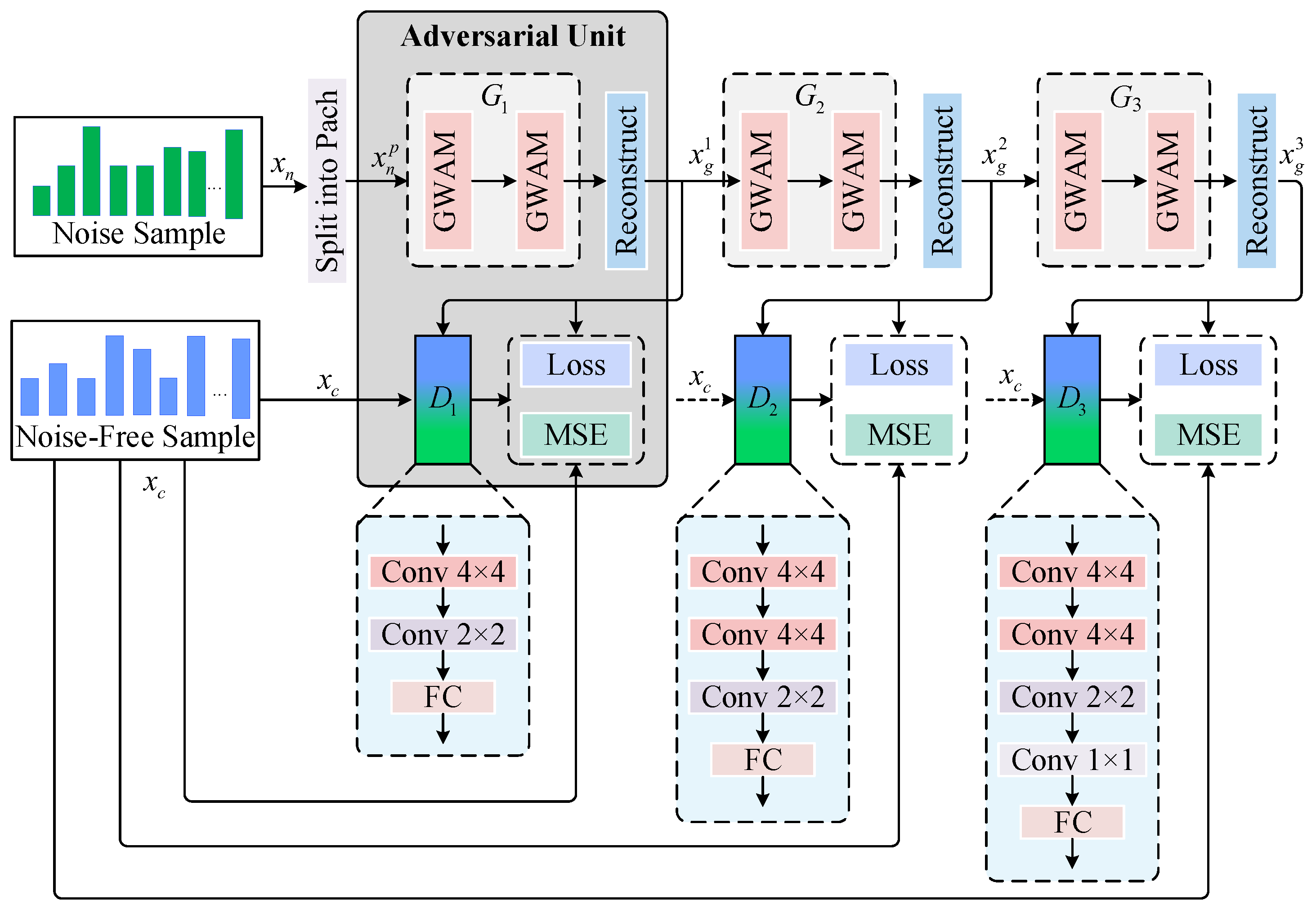
In non-stationary noise environments, high-quality reconstruction of gear fault features is hard to achieve based solely on the complex nonlinearity model with conventional regularization loss. Therefore, an adversarial mechanism is introduced as a new path to cooperate with the regularization loss for the improvement of feature reconstruction ability under noise interference. Considering that conventional adversarial training based on a single discriminator is insufficient to effectively constrain the details of acoustic signals at the global level due to potential issues such as vanishing gradients, mode collapse, and unstable convergence, a recursive adversarial mechanism is proposed, in which multiple discriminators are embedded within the multi-stage structure of the generator to perform a max-min game with equivalent GWAM units. This design decomposes the conventional mapping process into multi-stage adversarial learning by constructing auxiliary sub-GANs, which not only alleviates vanishing gradients but also facilitates the stable reconstruction of acoustic feature texture details in a “coarse-to-fine” recursive manner. The specific structures are illustrated in Figure 2.

Three discriminators with different structures $D_1,D_2,D_3$ impose constraints on the outputs generated by the GWAM at different levels of the generator, where $D_1,D_2,D_3$ are mainly composed of convolutional layers with different configurations and fully connected (FC) layers. Given an input spectrogram $X\in {\mathbb{R}}^{T\times F}$ and a convolution kernel $K\in {\mathbb{R}}^{W\times H}$, the convolution calculation process with stride s and padding p is defined as follows:

$$\begin{array}{c}\hfill {\mathrm{Conv}}_{W\times H}\left(X_{(i,j)}\right)=\phi (\sum _{m=0}^{W-1}\sum _{n=0}^{H-1}X(i+m,j+n)·K(m,n)),\end{array}$$

(13)

where $(i,j)$ denotes the location coordinates of the convolution kernel on the input feature map, $\phi (·)$ denotes the LeakyReLU activation function, and K denotes the convolution kernel with a size of $W\times H$. To align with the recursive adversarial denoising process in a “coarse-to-fine” manner, the discriminators are designed following a progressive strategy from weak to strong, with the specific parameter configurations detailed in

Table 1. Hyperparameters of discriminators.

Module	Structure	Hyperparameters
Discriminator-1	Conv 4 × 4	$W=4$, $H=4$, $s=4$, $p=\mathrm{False}$
	Conv 2 × 2	$W=2$, $H=2$, $s=2$, $p=\mathrm{False}$
	Fully Connected	$\mathrm{Layers}=1$
Discriminator-2	Conv 4 × 4	$W=4$, $H=4$, $s=4$, $p=\mathrm{False}$
	Conv 4 × 4	$W=4$, $H=4$, $s=4$, $p=\mathrm{False}$
	Conv 2 × 2	$W=2$, $H=2$, $s=2$, $p=\mathrm{False}$
	Fully Connected	$\mathrm{Layers}=1$
Discriminator-3	Conv 4 × 4	$W=4$, $H=4$, $s=4$, $p=\mathrm{False}$
	Conv 4 × 4	$W=4$, $H=4$, $s=4$, $p=\mathrm{False}$
	Conv 2 × 2	$W=2$, $H=2$, $s=2$, $p=\mathrm{False}$
	Conv 1 × 1	$W=1$, $H=1$, $s=1$, $p=\mathrm{False}$
	Fully Connected	$\mathrm{Layers}=1$

. $D_1$ is configured with a shallow nonlinear mapping that provides mild constraints, thereby stabilizing the early training stage, guiding the generator to eliminate prominent noise components, and preventing excessive penalization in the initial noise reduction phase:

$$\begin{array}{cc}\hfill D_1\left({\mathcal{X}}_1\right)& =\mathrm{FC}\left({\mathrm{Conv}}_{2\times 2}\left({\mathrm{Conv}}_{4\times 4}\left({\mathcal{X}}_1\right)\right)\right),\hfill \end{array}$$

(14)

where ${\mathcal{X}}_1$ represents either the clean signal or the denoised signal generated by $G_1$, and ${\mathrm{Conv}}_{2\times 2}$ and ${\mathrm{Conv}}_{4\times 4}$ denote convolutional layers with kernel sizes of $2\times 2$ and $4\times 4$, respectively. $D_2$ further increases the network depth based on the $D_1$ structure and cooperating with $G_2$ to extract finer details and periodic structural features, thus enhancing the feedback on intermediate denoising results:

$$\begin{array}{cc}\hfill D_2\left({\mathcal{X}}_2\right)& =\mathrm{FC}\left({\mathrm{Conv}}_{2\times 2}\left({\mathrm{Conv}}_{4\times 4}\left({\mathrm{Conv}}_{4\times 4}\left({\mathcal{X}}_2\right)\right)\right)\right),\hfill \end{array}$$

(15)

where ${\mathcal{X}}_2$ represents either the clean signal or the denoised signal generated by $G_2$. $D_3$, armed with the deepest structure to promote $G_3$ to, enforces constraints on the residual noise at the final stage, thereby restoring the periodic structures and texture details along the T-F dimension:

$$\begin{array}{cc}\hfill D_3\left({\mathcal{X}}_3\right)& =\mathrm{FC}\left({\mathrm{Conv}}_{1\times 1}\left({\mathrm{Conv}}_{2\times 2}\left({\mathrm{Conv}}_{4\times 4}\left({\mathrm{Conv}}_{4\times 4}\left({\mathcal{X}}_3\right)\right)\right)\right)\right),\hfill \end{array}$$

(16)

where ${\mathcal{X}}_3$ represents either the clean signal or the denoised signal generated by $G_3$. Such a recursive discriminative architecture with progressively increasing intensity ensures that the difficulty of discrimination matches that of generation, thereby enhancing the stability of model convergence and enabling a coarse-to-fine denoising process.

Recursive Generative Adversarial Denoising learning is a strategy that progressively enhances the denoising performance through the multi-level optimization of generated outputs, where the preceding result serves as the input for the subsequent stage, thereby achieving coarse-to-fine feature reconstruction and error correction. The overall structure of the proposed RGAD is shown in Figure 3. The generator and its corresponding discriminator ${(G_t,D_t)}_{t=1}^T$ ($T=3$) jointly function as a basic adversarial unit at each stage, and multiple adversarial units are then serially connected across multiple stages to form the overall RGAD structure. Specifically, the output of generator $G_t$ at one stage is fed as the input into the subsequent stage to achieve recursive denoising, where generator $G_t$ is mainly composed of two consecutive GWAMs, described in Section 3.1. At the same time, the output of $G_t$ is reconstructed from the patch level to the original T-F dimension and input into $D_t$ for adversarial discrimination and gradient feedback. The overall process can be expressed as

$$\begin{array}{c}\hfill x_g^t=G_t(x_g^{t-1};{\theta }_{G_t}),\end{array}$$

(17)

where $G_t$ receives the denoised output from the previous stage $x_g^{t-1}$ (where the input is the original noisy signal $x_n^p$, which is obtained through the patch partitioning operation, described in Section 3.1, when $t=1$) and generates the denoised signal $x_g^t$. ${\theta }_{G_t}$ denotes the learnable parameters of the generator at the i th stage in the recursive learning framework, where the parameters of the generator are entirely derived from the GWAM. The processed output $x_g^t$ is then passed into discriminator $D_t$, which evaluates its similarity to the target clean signal $x_c$:

$$\begin{array}{cc}\hfill & d_t^g=D_t(x_g^t;{\theta }_{D_t}),\hfill \\ \hfill & d_t^c=D_t(x_c;{\theta }_{D_t}),\hfill \end{array}$$

(18)

where $d_t^g$ denotes the output score of the discriminator for the denoised signal $x_g^t$, $d_t^c$ denotes the output score for the clean signal $x_c$, and ${\theta }_{D_t}$ represents the learnable parameters of the discriminator. During the adversarial process, the clean spectrum $x_c$ is used as the real sample and fed into the current discriminator to be distinguished from the generated denoised results. In this way, the discriminator can learn the statistical features of the true clean spectrogram and guide the generator to progressively produce outputs closer to the real distribution $x_c$ through discrimination error feedback. The final denoised output $x_g^3$ can thus be expressed as

$$\begin{array}{cc}\hfill & x_g^3=G_3(x_g^2,{\theta }_{G_3}),\hfill \\ \hfill & x_g^2=G_2(x_g^1,{\theta }_{G_2}),\hfill \\ \hfill & x_g^1=G_1(x_n^p,{\theta }_{G_1}),\hfill \\ \hfill & x_n^p=\mathrm{Patch}\left(x_n\right),\hfill \end{array}$$

(19)

where $\mathrm{Patch}(·)$ represents the patch partitioning operation introduced in Section 3.1.

This recursive generative adversarial strategy enables the model to effectively mitigate the vanishing gradient problem and significantly enhance its capability to restore the texture details of acoustic features in noise interference. The loss calculation and optimization strategy of RGAD are elaborated in detail in Section 3.3.

3.3. Loss Functions and Optimization Strategies

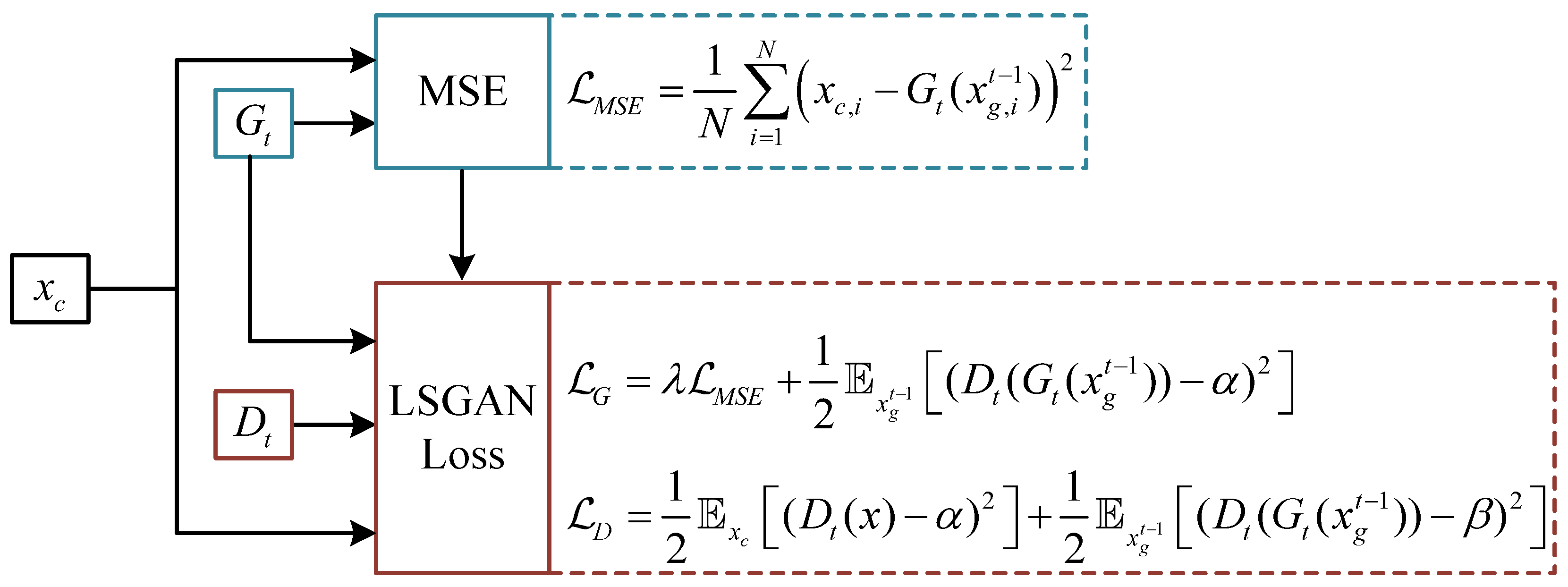
Considering that vanilla GANs are prone to suffer from vanishing gradients and training oscillation due to the sigmoid cross-entropy loss, the LSGAN substitutes the cross-entropy loss and form hybrid optimization objective with Mean Squared Error (MSE) to provide a stable training process in this work. The hybrid loss computation of the basic adversarial unit is illustrated in Figure 4. Specifically, the MSE is combined with the generator loss to impose a constraint with respect to the denoised spectrum in each adversarial unit. The modified loss function for the three-stage generator $G_t$ is formulated as

$$\begin{array}{cc}\hfill & {\mathcal{L}}_{G_1}=\lambda {\displaystyle \frac{1}{N}}\sum _{i=1}^N{\left(x_{c,i}-G_1\left(x_{n,i}^p\right)\right)}^2+{\displaystyle \frac{1}{2}}{\mathbb{E}}_{x_n}\left[{(D_1\left(G_1\left(x_n^p\right)\right)-\alpha )}^2\right],\hfill \end{array}$$

(20)

$$\begin{array}{cc}\hfill & {\mathcal{L}}_{G_2}=\lambda {\displaystyle \frac{1}{N}}\sum _{i=1}^N{\left(x_{c,i}-G_2\left(x_{g,i}^1\right)\right)}^2+{\displaystyle \frac{1}{2}}{\mathbb{E}}_{x_g^1}\left[{(D_2\left(G_2\left(x_g^1\right)\right)-\alpha )}^2\right],\hfill \end{array}$$

(21)

$$\begin{array}{cc}\hfill & {\mathcal{L}}_{G_3}=\lambda {\displaystyle \frac{1}{N}}\sum _{i=1}^N{\left(x_{c,i}-G_3\left(x_{g,i}^2\right)\right)}^2+{\displaystyle \frac{1}{2}}{\mathbb{E}}_{x_g^2}\left[{(D_3\left(G_3\left(x_g^2\right)\right)-\alpha )}^2\right],\hfill \end{array}$$

(22)

where N represents the number of samples, $x_{c,i}$ denotes the i-th clean sample, $x_{n,i}^p$ indicates the i-th noisy sample, $x_{g,i}^t$ represents the i-th denoised sample, and $\lambda$ is a weighting parameter set to 100 in this work to maintain an equilibrium between minimization and adversarial behavior according to previous studies on GANs. Meanwhile, it is worth noting that the Label Smoothing strategy is further introduced into the adversarial loss, which sets the real label to $\alpha =0.9$. By assigning the target value of real samples to a constant slightly less than 1, the risk of overfitting is effectively reduced and the training stability can be further improved. Correspondingly, the loss functions for the three-stage discriminator $D_t$ are as follows:

$$\begin{array}{cc}\hfill & {\mathcal{L}}_{D_1}={\displaystyle \frac{1}{2}}{\mathbb{E}}_{x_c}\left[{\left(D_1\left(x_c\right)-\alpha \right)}^2\right]+{\displaystyle \frac{1}{2}}{\mathbb{E}}_{x_n}\left[{(D_1\left(G_1\left(x_n^p\right)\right)-\beta )}^2\right],\hfill \end{array}$$

(23)

$$\begin{array}{cc}\hfill & {\mathcal{L}}_{D_2}={\displaystyle \frac{1}{2}}{\mathbb{E}}_{x_c}\left[{\left(D_2\left(x_c\right)-\alpha \right)}^2\right]+{\displaystyle \frac{1}{2}}{\mathbb{E}}_{x_g^1}\left[{(D_2\left(G_2\left(x_g^1\right)\right)-\beta )}^2\right],\hfill \end{array}$$

(24)

$$\begin{array}{cc}\hfill & {\mathcal{L}}_{D_3}={\displaystyle \frac{1}{2}}{\mathbb{E}}_{x_c}\left[{\left(D_3\left(x_c\right)-\alpha \right)}^2\right]+{\displaystyle \frac{1}{2}}{\mathbb{E}}_{x_g^2}\left[{(D_3\left(G_3\left(x_g^2\right)\right)-\beta )}^2\right],\hfill \end{array}$$

(25)

where $\beta$ represents the fake label and is set to $\beta =0$ in this work. The losses at each stage of the recursive three-stage training process are computed separately and optimized jointly in an end-to-end manner.

This paper employs a recursive learning framework to optimize the aforementioned loss functions. The core idea of recursion is to replace the complex direct mapping with a multi-stage indirect mapping process, achieving progressive denoisation through multiple simplified denoising modules. Specifically, we utilize the Adam optimizer to independently optimize the three sets of generators and discriminators ${(G_t,D_t)}_{t=1}^T,T=3$. Within each group, $G_t$ and $D_t$ share an optimizer and are updated simultaneously to maintain the dynamic balance of the adversarial process. It should be noted that this recursive architecture not only prevents error accumulation but also helps mitigate the gradient vanishing problem caused by network depth. The specific update rules for the generator parameters are as follows:

$$\begin{array}{cc}\hfill & {\theta }_{G_1}\leftarrow {\theta }_{G_1}-{\eta }_{\mathrm{adam}}\left({\displaystyle \frac{\partial {\mathcal{L}}_{{\mathrm{G}}_1}}{{\theta }_{G_1}}}+{\displaystyle \frac{\partial {\mathcal{L}}_{{\mathrm{G}}_2}}{{\theta }_{G_1}}}+{\displaystyle \frac{\partial {\mathcal{L}}_{{\mathrm{G}}_3}}{{\theta }_{G_1}}}\right),\hfill \\ \hfill & {\theta }_{G_2}\leftarrow {\theta }_{G_2}-{\eta }_{\mathrm{adam}}\left({\displaystyle \frac{\partial {\mathcal{L}}_{{\mathrm{G}}_2}}{{\theta }_{G_2}}}+{\displaystyle \frac{\partial {\mathcal{L}}_{{\mathrm{G}}_3}}{{\theta }_{G_2}}}\right),\hfill \\ \hfill & {\theta }_{G_3}\leftarrow {\theta }_{G_3}-{\eta }_{\mathrm{adam}}\left({\displaystyle \frac{\partial {\mathcal{L}}_{{\mathrm{G}}_3}}{{\theta }_{G_3}}}\right),\hfill \end{array}$$

(26)

where ${\eta }_{\mathrm{adam}}$ represents the Adam optimizer with a fixed learning rate of $\eta =0.0002$. This configuration plays a crucial role in maintaining the delicate balance between the generators and discriminators throughout the adversarial training process. Similarly, the generator also updates its parameters along the gradient descent direction, expressed as

$$\begin{array}{cc}\hfill & {\theta }_{D_1}\leftarrow {\theta }_{D_1}-{\eta }_{\mathrm{adam}}\left({\displaystyle \frac{\partial {\mathcal{L}}_{{\mathrm{D}}_1}}{{\theta }_{D_1}}}+{\displaystyle \frac{\partial {\mathcal{L}}_{{\mathrm{D}}_2}}{{\theta }_{D_1}}}+{\displaystyle \frac{\partial {\mathcal{L}}_{{\mathrm{D}}_3}}{{\theta }_{D_1}}}\right),\hfill \\ \hfill & {\theta }_{D_2}\leftarrow {\theta }_{D_2}-{\eta }_{\mathrm{adam}}\left({\displaystyle \frac{\partial {\mathcal{L}}_{{\mathrm{D}}_2}}{{\theta }_{D_2}}}+{\displaystyle \frac{\partial {\mathcal{L}}_{{\mathrm{D}}_3}}{{\theta }_{D_2}}}\right),\hfill \\ \hfill & {\theta }_{D_3}\leftarrow {\theta }_{D_3}-{\eta }_{\mathrm{adam}}\left({\displaystyle \frac{\partial {\mathcal{L}}_{{\mathrm{D}}_3}}{{\theta }_{D_3}}}\right).\hfill \end{array}$$

(27)

3.4. Overall RGAD-Based ABD Framework

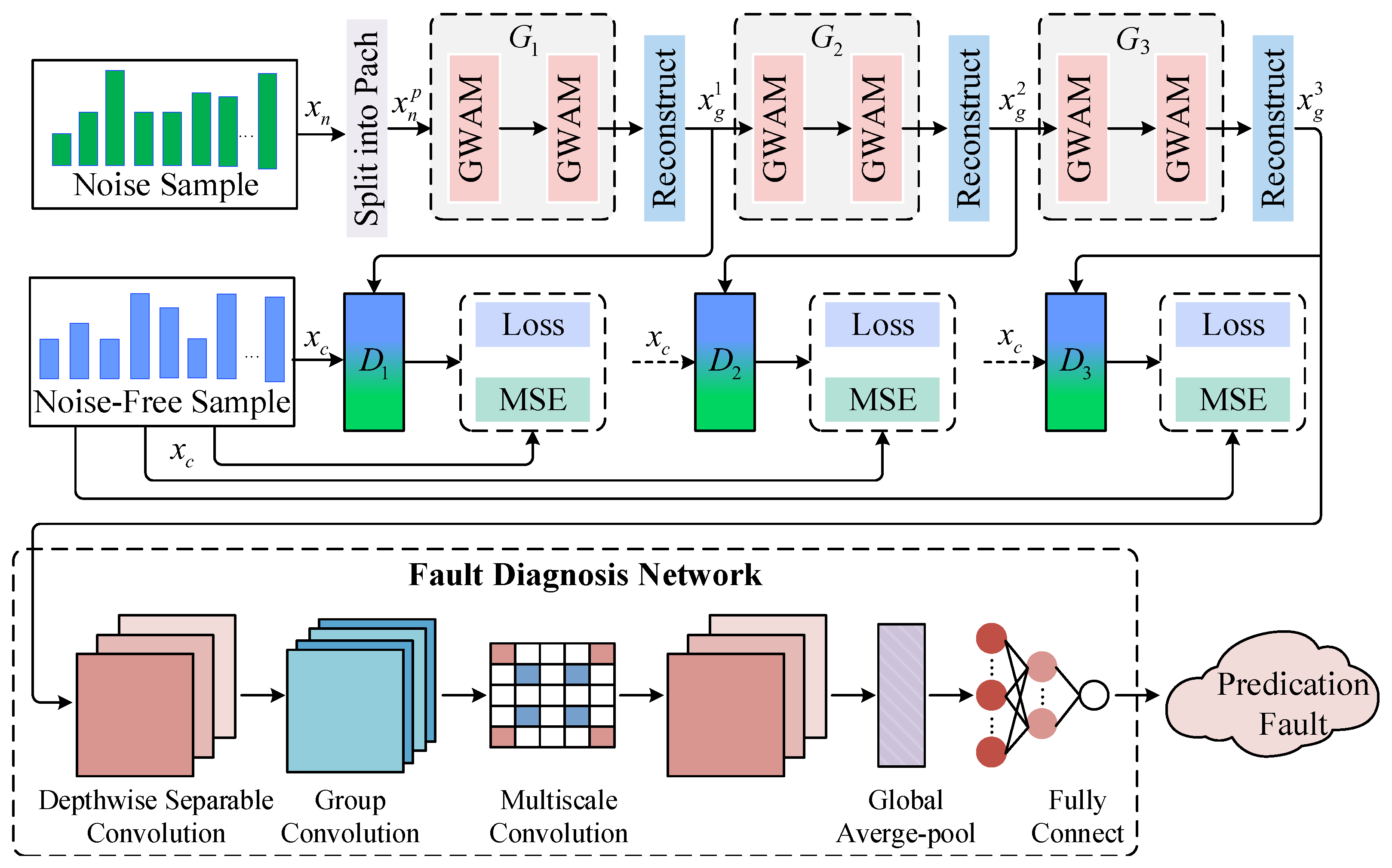
The proposed RGAD is integrated with the fault diagnosis network (FDN) to construct the complete RGAD-based ABD framework. The overall structure of the framework is shown in Figure 5. Firstly, the original gear rotational acoustic signal collected under noisy conditions is transformed into a spectral representation $x_n$ and then fed into RGAD to progressively remove noise components and gradually reconstruct periodic structural features and texture details. Subsequently, the denoised spectrum $x_g^3$ output by the final-stage generator $G_3$ is input into the FDN for sequential fault feature extraction and classification.

As shown in the lower part of Figure 5, the FDN mainly consists of depthwise separable convolution, group convolution, multi-scale convolution, global pooling, and a fully connected layer. The first three components of the network form the feature extraction module, which is designed to capture the periodic pulse patterns and time–frequency harmonic distributions associated with fault characteristics, while the global pooling and fully connected layers are utilized for fault classification based on the extracted features.

3.5. Fault Diagnosis Procedure of the Proposed Framework

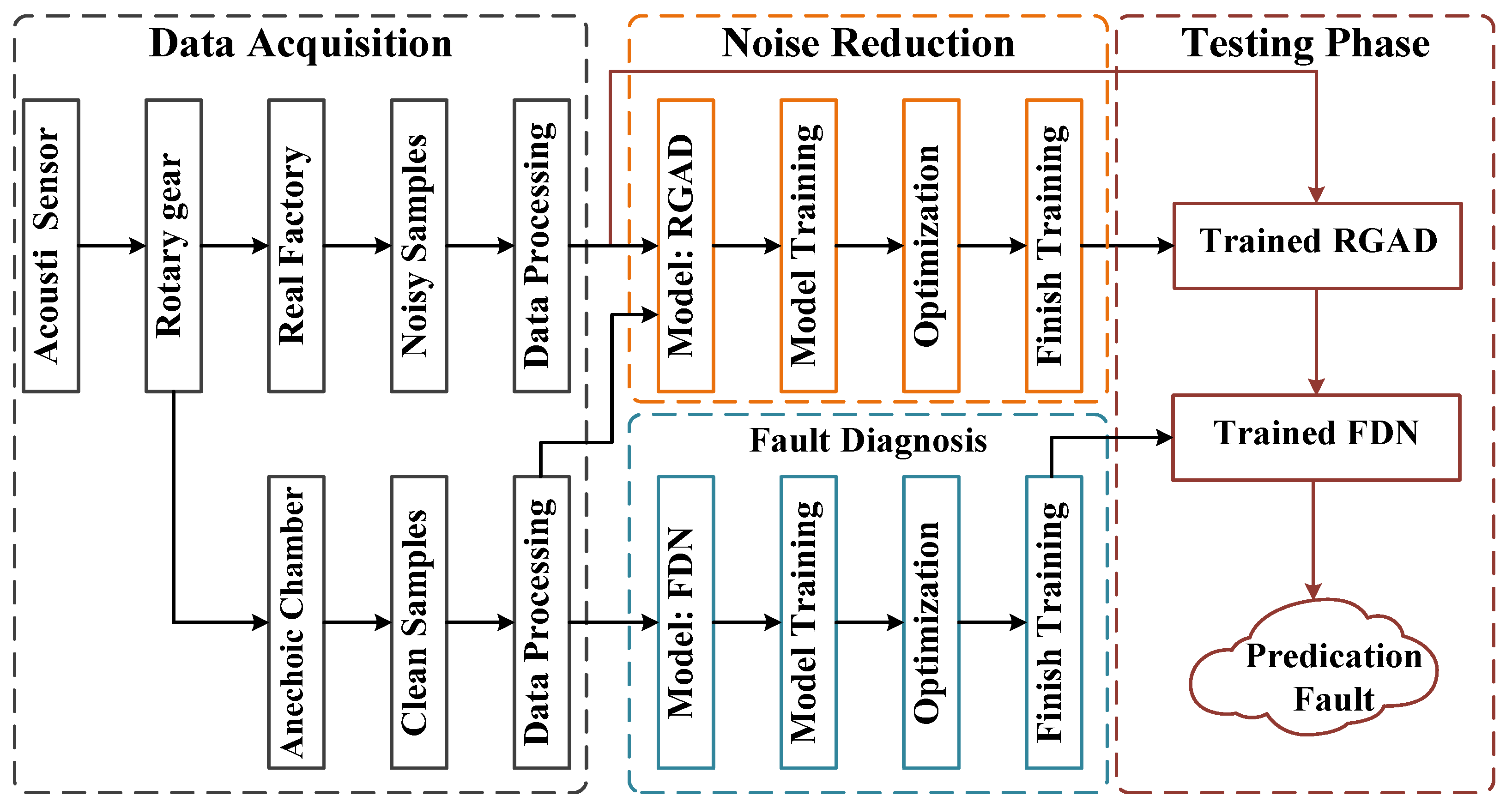
The fault diagnosis process of the RGAD-based ABD framework is shown in Figure 6. The original gear rotational acoustic signal is first collected in real factory environments and in a semi-anechoic chamber, respectively, using the established acoustic measurement platform (for details, see Section 4.1.1 and Section 4.1.2). Subsequently, the acquired one-dimensional waveform signal is preprocessed into a two-dimensional spectrum through the method presented in Section 4.1.3, which is utilized for training, validation, and testing. During the training stage, noise suppression and fault diagnosis are treated as entirely independent processes: the spectrum containing non-stationary noise is exclusively utilized in the RGAD model for supervised learning, with the clean spectrum serving as the target, while the clean spectrum is independently employed for the FDN. During the testing phase, the trained RGAD model and FDN network are cascaded to facilitate gear fault pattern recognition based on acoustic samples collected in real industrial environments.

4. Experiments

In this section, we first present the experimental setup, including the experimental conditions, data acquisition process, and implementation details. Subsequently, a series of ablation studies and comparative experiments are conducted to evaluate the effectiveness of the proposed RGAD method against non-stationary noise interference and to further demonstrate the superiority of the RGAD-based ABD framework for gear fault diagnosis under real industrial scenarios.

4.1. Experimental Setup

4.1.1. Experiment System

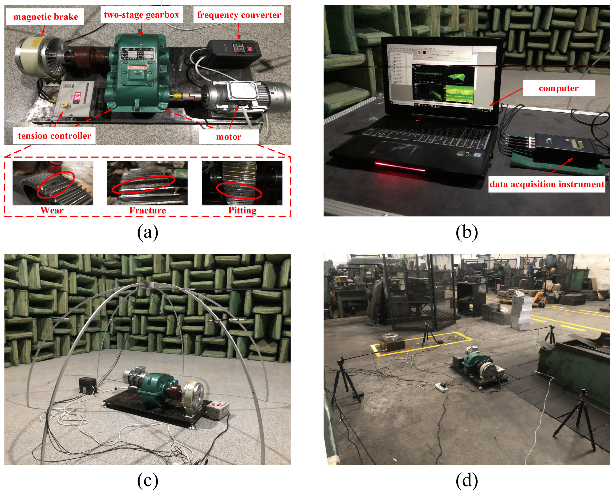
The experimental investigations were conducted on a self-designed gearbox test platform, as illustrated in Figure 7a–d. The test system can be divided into three major components: (i) the gearbox test bench, (ii) the acoustic measurement setup, and (iii) the data acquisition and recording module. The gearbox test bench is driven by a variable-frequency motor controlled by a frequency inverter, and it is mechanically loaded through a tension controller and a magnetic brake. To capture the acoustic response, a four-channel microphone array is deployed around the gearbox. The microphones are mounted in either a hemispherical or rectangular enclosing configuration, with symmetric placement that complies with the ISO 3745:2012 standard. The acoustic signals are transmitted via Bayonet Nut Connectors (BNCs) to a multi-channel data acquisition instrument, ensuring stable and synchronized signal collection. Finally, the data are stored in .WAVformat through a dedicated recording software package for subsequent analysis.

Accordingly, experimental datasets comprising clean acoustic signals and noise-contaminated acoustic signals were, respectively, established. The dataset covers four gear health states under three different rotational speeds, including one normal condition and three representative fault types. For each health state, 35 four-channel audio recordings of 60 s were collected. The recordings were then divided into training, validation, and test sets with an approximate ratio of 70%, 15%, and 15%, respectively. To facilitate effective modeling in acoustic signal processing tasks, each 60 s audio file in .WAV format was further segmented into non-overlapping 1 s segments, thereby ensuring sufficient sample quantity in each dataset.

4.1.2. Data Preprocessing

In the experiments, the acoustic signals from both datasets were sampled at a frequency of 16 kHz. The signals were framed using a 64 ms Hamming window with 50% overlap between consecutive frames. For each frame, a Mel-frequency filter bank consisting of 40 filters was applied, producing a 40-dimensional feature vector. Consequently, each 1 s acoustic sample was transformed into a two-dimensional Mel-frequency spectrum, which characterizes the time–frequency (T-F) representation of the gear acoustic signals. To facilitate model training, the Mel-frequency spectra of both clean and noise-contaminated signals were normalized by scaling their amplitudes into the range $[-1,1]$.

4.1.3. Evaluation Metrics

The primary objective of RGAD is to eliminate non-stationary noise components from the input acoustic signals through the proposed recursive adversarial strategy while simultaneously refining periodic structural features and texture details that may be obscured by noise, thereby facilitating improved subsequent diagnostic performance. To quantitatively evaluate the effectiveness of this strategy, two widely adopted similarity metrics, Mean Squared Error (MSE) and Peak Signal-to-Noise Ratio (PSNR), are introduced for assessing the signal-level denoising quality. Furthermore, the diagnostic accuracy is employed to evaluate the performance at the task level.

MSE quantifies the global statistical error by calculating the average squared difference between the denoised spectrum and the clean target spectrum. It provides a direct measure of the overall deviation, where a lower MSE value indicates a smaller error and reflects superior denoising performance by signifying a closer approximation to the target clean signal. The MSE between the denoised signal $x_g^3$ and the clean reference $x_c$, both of size, is defined as

$$\begin{array}{c}\hfill {\displaystyle \frac{1}{N}}\sum _{i=1}^N{\left(x_{c,i}-x_{g,i}^3\right)}^2.\end{array}$$

(28)

The PSNR is derived from the MSE and serves as a logarithmic measure of reconstruction fidelity. It is computed as the ratio between the maximum possible power of a signal and the power of the introduced noise (represented by the MSE). An increased PSNR value suggests that the noise power in the denoised signal is comparatively lower relative to the peak power of the clean signal, thus indicating enhanced denoising quality and better preservation of the signal’s structural integrity. The PSNR (in decibels, dB) is defined as

$$\begin{array}{c}\hfill \mathrm{PSNR}=10·{log}_{10}\left({\displaystyle \frac{{\mathrm{MAX}}^2}{\mathrm{MSE}}}\right),\end{array}$$

(29)

where $\mathrm{MAX}$ represents the maximum possible value in the clean signal $x_c$ and is defined as 1 in the normalized spectrum.

While the MSE and PSNR evaluate the quality of the denoised signal itself, the ultimate objective is to improve the performance of downstream fault diagnosis tasks. Diagnostic accuracy is thus introduced to measure the effectiveness of the denoising process at the task level. It is defined as the ratio of correctly classified samples to the total number of samples tested, when the diagnosis is performed on the denoised signals. Higher accuracy signifies that the denoising process has more effectively retained or enhanced the discriminative features necessary for reliable classification. The accuracy is calculated as

$$\begin{array}{c}\hfill \mathrm{Accuracy}={\displaystyle \frac{TP+TN}{TP+TN+FP+FN}}\times 100\%,\end{array}$$

(30)

where $TP$ (True Positives) represents the number of faulty samples correctly identified as faulty; $TN$ (True Negatives) represents the number of normal samples correctly identified as normal; $FP$ (False Positives) represents the number of normal samples incorrectly identified as faulty; and $FN$ (False Negatives) represents the number of faulty samples incorrectly identified as normal.

4.2. Analysis of RGAD

The effectiveness of RGAD is comprehensively evaluated at the statistical level using both the MSE and PSNR metrics, with the experimental results summarized in

Table 2. MSE and PSNR values between RGAD-denoised acoustic signals and clean acoustic signals.

Method	MSE	PSNR
Original	0.07892	11.08
Adversarial Unit 1	0.01734	17.61
Adversarial Unit 2	0.01654	17.81
Adversarial Unit 3 (final output)	0.01644	17.84

. It is easy to observe from Table 2 that the MSE between the spectrum processed by the three adversarial units and the clean spectrum consistently decreases, while the PSNR correspondingly increases within the recursive adversarial framework. This verifies the effectiveness of the recursive strategy at the global statistical level.

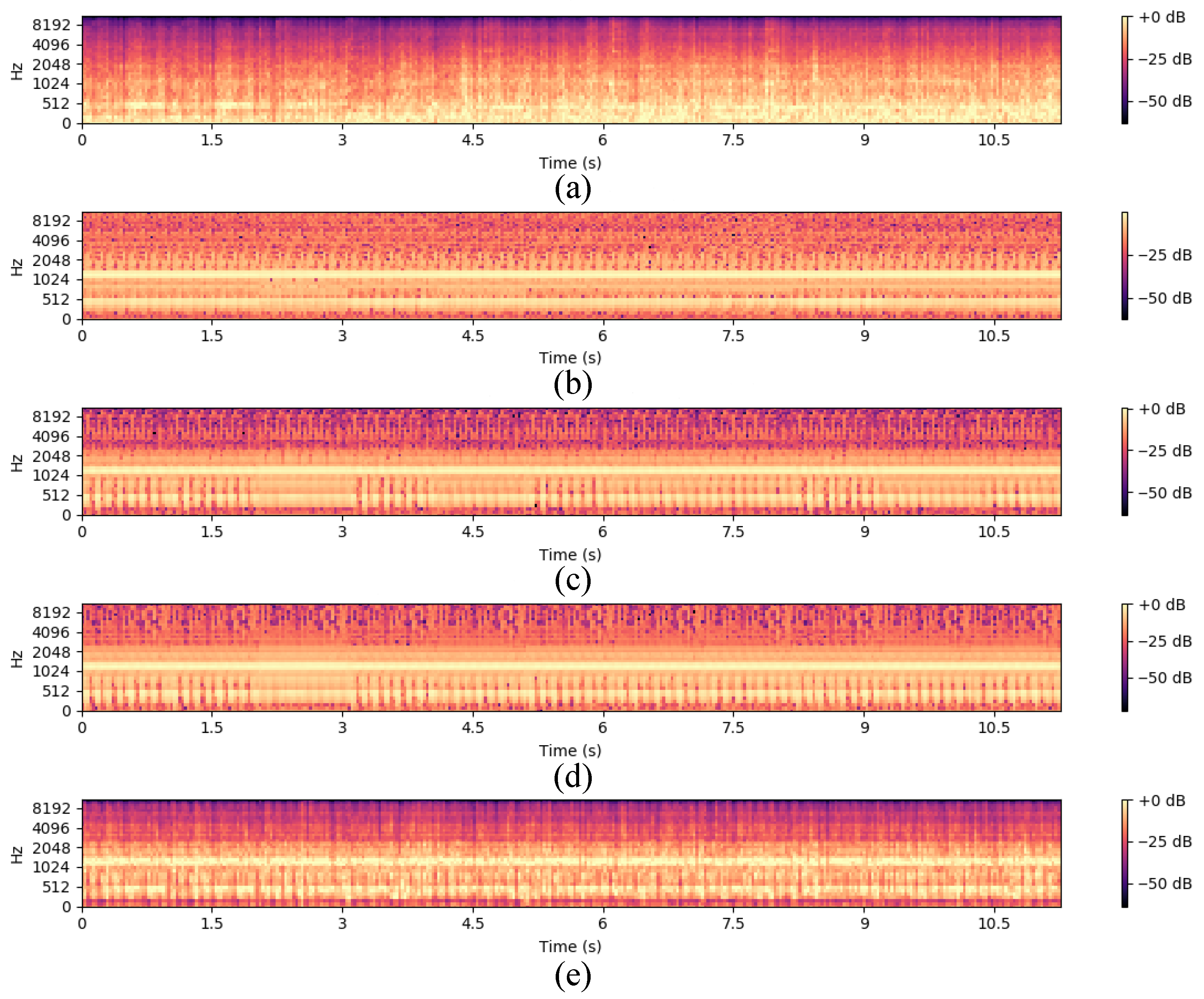
To provide a more intuitive understanding of how the recursive adversarial strategy in RGAD removes non-stationary noise and restores periodic and sparse features associated with fault patterns that are masked by noise, we conducted a visualization experiment on selected test samples, as shown in Figure 8. By comparing Figure 8a and Figure 8e, it can be observed that the meshing frequencies in the range of 200 to 500 Hz, along with their higher-order harmonics around 1000 to 1500 Hz, are obscured by non-stationary noise. The purpose of RGAD is to progressively eliminate such non-stationary industrial noise through the recursive adversarial framework and recover the obscured features in a coarse-to-fine manner. As observed in the outputs of adversarial units 1 to 3 (i.e., Figure 8b–d), it can be found that in the frequency domain, although the reconstruction performance of RGAD is limited in frequency components above 3000 Hz, the noise-interference characteristics are progressively restored in the mesh frequency and high-harmonic frequency regions. Meanwhile, the periodic structure of the gear acoustic signal along the time axis is clearly reconstructed. Further analysis incorporating time–frequency information reveals that the texture details present in the clean spectrum are also gradually recovered by RGAD. The above observations provide strong evidence for the effectiveness of RGAD in addressing non-stationary noise interference at a microscopic level.

4.3. Ablation Experiments

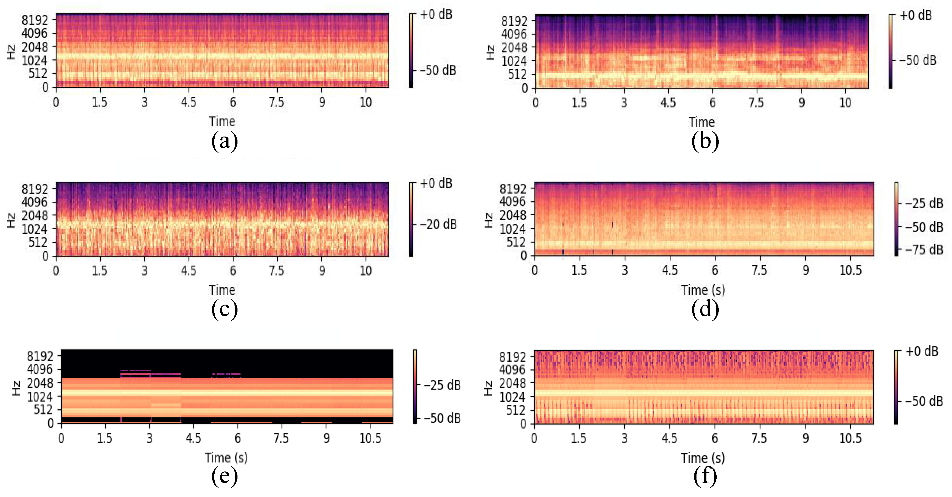
As a core component of RGAD, the designed recursive discriminative architecture functions to refine the denoised spectrum in a coarse-to-fine manner through progressive guidance. To further evaluate the effectiveness of this progressive adversarial mechanism, ablation studies are performed. Specifically, the discriminators with three different structures in the recursive discriminative architecture are removed or configured to the identical structure (e.g., all adopting $D_1$) to compare with the proposed RGAD in denoising performance and diagnostic accuracy. It can be clearly observed from

Table 3. RGAD ablation experiment results, where Accuracy represents the fault diagnosis accuracy rate (%).

Method	Unit 1-MSE	Unit 2-MSE	Unit 3-MSE	PSNR	Accuracy
Regularization loss	0.01785	0.01669	0.01651	17.82	95.28
Equivalent discriminator $D_1$	0.01966	0.01821	0.01766	17.53	91.33
Equivalent discriminator $D_2$	0.02529	0.02368	0.01655	17.81	94.86
Equivalent discriminator $D_3$	0.01665	0.01647	0.01649	17.83	96.52
RGAD (ours)	0.01734	0.01654	0.01644	17.84	97.31

that an inappropriate discriminative architecture adversely affects the overall recursive process. In particular, after all adversarial units are equipped with the discriminator of the $D_3$ structure, the performance of adversarial unit 3 is attenuated, and its similarity metrics with the clean target spectrum is lower than that of adversarial unit 2. This is because the output in the early stage is over-constrained, which blocks recursive propagation in the later stage. Conversely, once a shallow discriminator with a structure of $D_1$ is adopted in the later stage, the final output denoised spectrum following the recursive process shows a significant difference from the clean target spectrum in terms of similarity evaluation metrics. Meanwhile, the medium-strength discriminator, configured with the D2 structure throughout the recursive process, can achieve intermediate performance between the two aforementioned cases. Different from that, constraining the recursive process solely through the regularization loss rather than the adversarial loss is beneficial for the recursive behavior and denoising results, but it suffers from the over-smoothing issue, as illustrated in Figure 9. Combined with the accuracy indicators in Table 3, it can be found that the lack of spectral texture details causes the loss of diagnostic information, thereby resulting in reduced diagnostic accuracy compared to most recursive models based on the adversarial mechanism under the FDN with the same structure and parameter configuration. Furthermore, by comparing the sampling visualization denoising spectrum and diagnostic accuracy from $D_1$ to $D_3$ in Figure 9 and Table 3, it is easy to find that improved restoration quality of spectral texture details leads to a corresponding increase in diagnostic accuracy. The proposed RGAD method, benefiting from its superior capability in reconstructing spectral texture details, achieves the highest diagnostic accuracy. These experimental results confirm the positive correlation between the preservation of spectral texture details and diagnostic accuracy.

Considering that the theoretical computational complexity of the inference stage is an objective indicator to evaluate the efficiency of the model, we focus exclusively on evaluating the computational cost after model training. As shown in

Table 4. Computational costs of different methods.

Method	FLOPs	Parameters	Inference/Sample
Regularization loss	1,569,138	2,341,718	0.30 ms
Equivalent discriminator $D_1$	1,569,138	2,344,972	0.30 ms
Equivalent discriminator $D_2$	1,569,138	2,420,524	0.30 ms
Equivalent discriminator $D_3$	1,569,138	2,496,172	0.30 ms
RGAD (ours)	1,569,138	3,980,684	0.30 ms

, since the discriminator is not invoked during the testing phase, all methods exhibit identical FLOPs and single-sample inference time. Furthermore, although the proposed method has the highest parameter count among the compared approaches, it remains under 4M, reflecting a lightweight structure and indicating strong potential for deployment on edge devices and in practical applications. Meanwhile, the proposed method achieves the best performance by slightly increasing the number of parameters compared to other approaches, demonstrating that the trade-off between complexity and performance is well justified.

4.4. Compared with Other Methods

To further evaluate the superiority of the proposed RGAD, a comparative analysis is conducted with the methods outlined in the Introduction. Specifically, the comparison encompasses the traditional denoising filtering approach based on statistical property modeling, as well as the classical generative adversarial denoising method widely adopted in speech enhancement tasks. A detailed description of these methods is provided as follows:

(1) Least Mean Square (LMS) [19] is a traditional adaptive filtering algorithm based on the Wiener filter, and it has been widely applied to non-stationary signal processing.

(2) Recursive Least Squares (RLS) [20] is a representative adaptive filtering algorithm derived from Kalman filtering theory [21], which provides superior noise tracking and estimation performance for non-stationary signals.

(3) TF-Masking [30] is a novel speech enhancement approach that innovatively employs the generative adversarial mechanism to construct masks in the time–frequency domain, thereby enabling the effective suppression of noise components under non-stationary conditions.

(4) GAN-$L_1$ [27] represents a classical generative adversarial denoising framework, which effectively integrates generative adversarial loss with $L_1$ regularization loss to achieve superior performance in suppressing non-stationary noise.

Table 5. The MSE and PSNR of the denoised spectrum and target spectrum for different methods, along with the fault diagnostic accuracy.

Method	MSE	PSNR	Accuracy
LMS	0.05559	12.55	31.99
RLS	0.04535	13.43	79.78
TF-Masking	0.03892	14.10	53.47
GAN-L1	0.01766	17.53	95.41
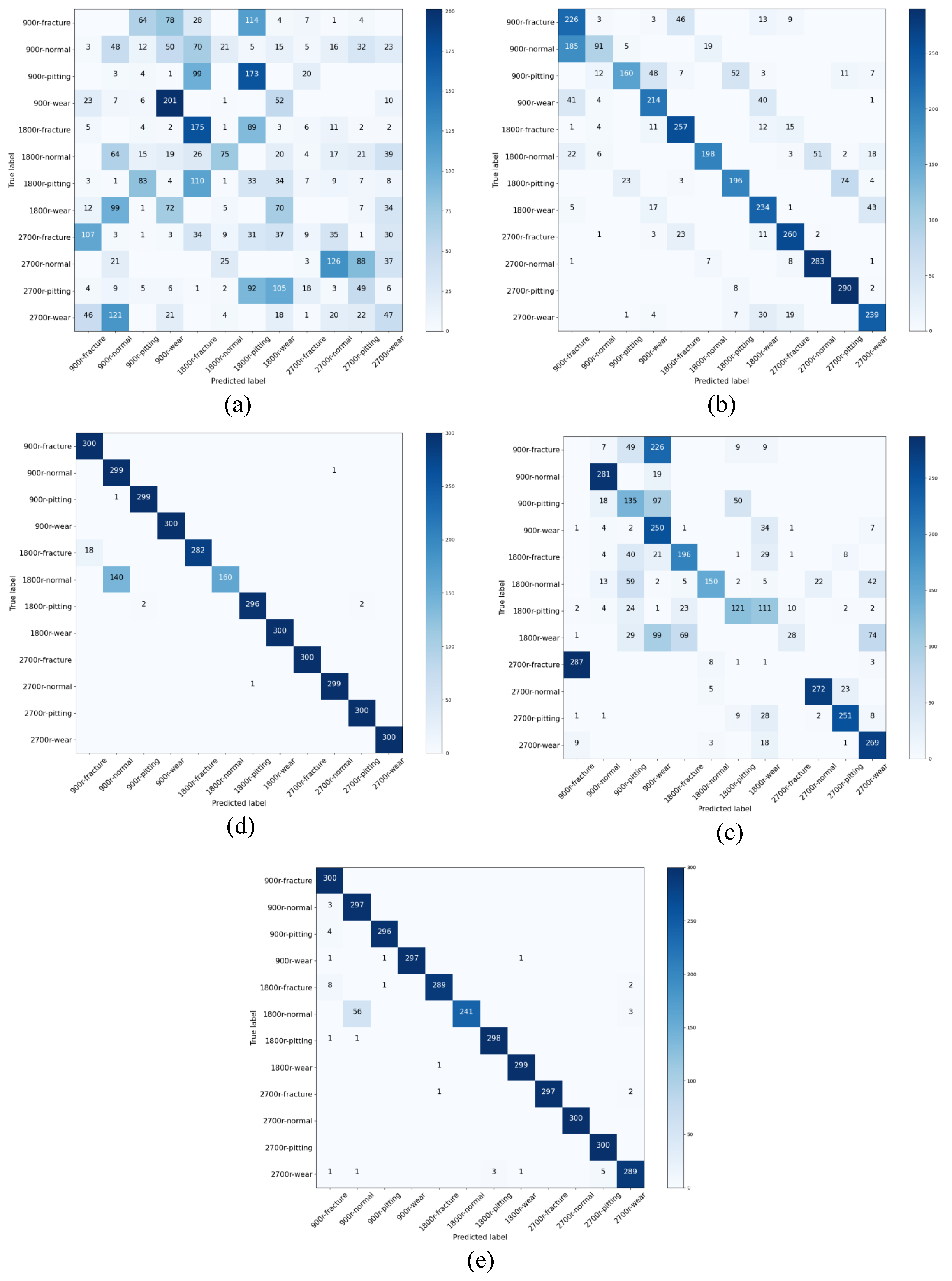
RGAD (ours)	0.01644	17.84	97.31

presents the comparative results between RGAD and the aforementioned methods in denoising performance and diagnostic accuracy. It can be seen that the adversarial method outperforms the traditional filtering approaches based on statistical property modeling in terms of the global similarity index related to noise reduction performance. To further analyze from the perspective of spectral reconstruction, the denoising outcomes of these approaches are sampled for visualized comparison, as shown in Figure 10. It is clear that the spectra recovered by LMS, RLS, and TF-Masking maintain well-preserved texture details while exhibiting varying degrees of periodic structure loss. Specifically, LMS and TF-Masking fail to accurately reconstruct the periodic structural features of the signal in the high-order harmonic frequency band (approximately 1000–1500 Hz), whereas RLS demonstrates suboptimal performance in recovering periodic information around the meshing frequency (500 Hz). By integrating the diagnostic accuracy presented in Table 3, it can be observed that RLS, which demonstrates superior periodic structure reconstruction capability within the high-order harmonic frequency band, significantly outperforms LMS and T-F masking in terms of diagnostic performance. This indicates that higher-order harmonics within the frequency range of approximately 1000 to 1500 Hz carry critical information associated with the gear’s health state, thereby having a significant impact on diagnostic accuracy. This phenomenon can also be further confirmed by the performance of GAN-$L_1$, where the second-highest diagnostic accuracy is achieved as a result of preserving complete periodic structure information in the higher-order harmonic frequency band despite being affected by over-smoothing issues. Different from that, the proposed RGAD effectively balances the reconstruction of periodic structural features with the restoration of fine texture details, thereby achieving the best diagnostic performance (as shown in Figure 11). This further illustrates the superiority of RGAD for ABD tasks under non-stationary noise interference conditions in real industrial scenarios.

5. Conclusions

This article proposes a novel RGAD-based ABD framework for gear fault diagnosis in real industrial noise conditions. As the backbone of the model, the GWAM-based generator is capable of effectively reconstructing the periodic structural characteristics of gear acoustic signals under non-stationary noise interference through recursively capturing T-F global dependencies. The adversarial mechanism based on recursive discriminator architecture significantly enhances reconstruction quality of texture details for acoustic features while effectively preventing the vanishing gradient problem in adversarial learning. Through the above design, the non-stationary noise is effectively suppressed and the high-quality reconstruction of the periodic structure and texture details of the gear rotation acoustic signal can be achieved in a coarse-to-fine manner. Finally, by integrating RGAD with a diagnosis module FDN, a complete RGAD-based ABD framework is well-established for gear fault diagnosis in real industrial scenarios. Experimental results under real industrial background noise conditions demonstrate that the proposed RGAD-based ABD franework achieves superior noise suppression and gear fault diagnosis performance.

References

1. Chen, C.; Shen, F.; Xu, J.; Yan, R. Probabilistic latent semantic analysis-based gear fault diagnosis under variable working conditions. IEEE Trans. Instrum. Meas. 2019, 69, 2845–2857. [Google Scholar] [CrossRef]
2. Yao, Y.; Gui, G.; Yang, S.; Zhang, S. A recursive multi-head self-attention learning for acoustic-based gear fault diagnosis in real-industrial noise condition. Eng. Appl. Artif. Intell. 2024, 133, 108240. [Google Scholar] [CrossRef]
3. Yao, Y.; Gui, G.; Yang, S.; Zhang, S. A recursive denoising learning for gear fault diagnosis based on acoustic signal in real industrial noise condition. IEEE Trans. Instrum. Meas. 2021, 70, 3524015. [Google Scholar] [CrossRef]
4. Rezaei, A.; Dadouche, A.; Wickramasinghe, V.; Dmochowski, W. A comparison study between acoustic sensors for bearing fault detection under different speed and load using a variety of signal processing techniques. Tribol. Trans. 2011, 54, 179–186. [Google Scholar] [CrossRef]
5. Peng, B.; Li, D.; Wang, K.I.K.; Abdulla, W.H. Acoustic-Based Industrial Diagnostics: A Scalable Noise-Robust Multiclass Framework for Anomaly Detection. Processes 2025, 13, 544. [Google Scholar] [CrossRef]
6. Scanlon, P.; Kavanagh, D.F.; Boland, F.M. Residual life prediction of rotating machines using acoustic noise signals. IEEE Trans. Instrum. Meas. 2012, 62, 95–108. [Google Scholar] [CrossRef]
7. Zhang, D.; Stewart, E.; Entezami, M.; Roberts, C.; Yu, D. Intelligent acoustic-based fault diagnosis of roller bearings using a deep graph convolutional network. Measurement 2020, 156, 107585. [Google Scholar] [CrossRef]
8. Hassan, A.; Hashem, A.F.; Sayed, A.; Kayed, M. Physics-guided deep learning for acoustic-based fault diagnosis. Int. J. Engine Res. 2025. [Google Scholar] [CrossRef]
9. Hou, J.; Jiang, W.; Lu, W. Application of a near-field acoustic holography-based diagnosis technique in gearbox fault diagnosis. J. Vib. Control 2013, 19, 3–13. [Google Scholar] [CrossRef]
10. Yao, Y.; Zhang, S.; Yang, S.; Gui, G. Learning attention representation with a multi-scale CNN for gear fault diagnosis under different working conditions. Sensors 2020, 20, 1233. [Google Scholar] [CrossRef]
11. Yao, Y.; Wang, H.; Li, S.; Liu, Z.; Gui, G.; Dan, Y.; Hu, J. End-to-end convolutional neural network model for gear fault diagnosis based on sound signals. Appl. Sci. 2018, 8, 1584. [Google Scholar] [CrossRef]
12. Glowacz, A. Acoustic based fault diagnosis of three-phase induction motor. Appl. Acoust. 2018, 137, 82–89. [Google Scholar] [CrossRef]
13. Glowacz, A. Fault detection of electric impact drills and coffee grinders using acoustic signals. Sensors 2019, 19, 269. [Google Scholar] [CrossRef]
14. Glowacz, A. Acoustic fault analysis of three commutator motors. Mech. Syst. Signal Process. 2019, 133, 106226. [Google Scholar] [CrossRef]
15. Ebrahimkhanlou, A.; Dubuc, B.; Salamone, S. A generalizable deep learning framework for localizing and characterizing acoustic emission sources in riveted metallic panels. Mech. Syst. Signal Process. 2019, 130, 248–272. [Google Scholar] [CrossRef]
16. Boll, S. Suppression of acoustic noise in speech using spectral subtraction. IEEE Trans. Acoust. Speech Signal Process. 2003, 27, 113–120. [Google Scholar] [CrossRef]
17. Scalart, P. Speech enhancement based on a priori signal to noise estimation. In Proceedings of the 1996 IEEE International Conference on Acoustics, Speech, and Signal Processing Conference Proceedings, Atlanta, GA, USA, 9 May 1996; Volume 2, pp. 629–632. [Google Scholar]
18. Ephraim, Y.; Malah, D. Speech enhancement using a minimum-mean square error short-time spectral amplitude estimator. IEEE Trans. Acoust. Speech Signal Process. 2003, 32, 1109–1121. [Google Scholar] [CrossRef]
19. Haykin, S.; Widrow, B. LEAST-MEAN-SQUARE ADAPTIVE FILTERS; Wiley Online Library: Hoboken, NJ, USA, 2003. [Google Scholar]
20. Martinek, R.; Vanus, J.; Kelnar, M.; Bilik, P.; Zidek, J. Application of recursive least square algorithm to adaptive channel equalization. In Proceedings of the Measurement in Research and Industry, Shenzhen, China, 27–28 December 2015. [Google Scholar]
21. Diniz, P.S. Adaptive Filtering; Springer: Berlin/Heidelberg, Germany, 1997; Volune 4. [Google Scholar]
22. Shao, Y.; Srinivasan, S.; Jin, Z.; Wang, D. A computational auditory scene analysis system for speech segregation and robust speech recognition. Comput. Speech Lang. 2010, 24, 77–93. [Google Scholar] [CrossRef]
23. Narayanan, A.; Wang, D. Investigation of speech separation as a front-end for noise robust speech recognition. IEEE/ACM Trans. Audio Speech Lang. Process. 2014, 22, 826–835. [Google Scholar] [CrossRef]
24. Xu, Y.; Du, J.; Dai, L.R.; Lee, C.H. A regression approach to speech enhancement based on deep neural networks. IEEE/ACM Trans. Audio Speech Lang. Process. 2014, 23, 7–19. [Google Scholar] [CrossRef]
25. Seltzer, M.L.; Yu, D.; Wang, Y. An investigation of deep neural networks for noise robust speech recognition. In Proceedings of the 2013 IEEE International Conference on Acoustics, Speech and Signal Processing, Vancouver, BC, Canada, 26–31 May 2013; pp. 7398–7402. [Google Scholar]
26. Pascual, S.; Bonafonte, A.; Serra, J. SEGAN: Speech enhancement generative adversarial network. arXiv 2017, arXiv:1703.09452. [Google Scholar] [CrossRef]
27. Pandey, A.; Wang, D. On adversarial training and loss functions for speech enhancement. In Proceedings of the 2018 IEEE International Conference on Acoustics, Speech and Signal Processing (ICASSP), Calgary, AB, Canada, 15–20 April 2018; pp. 5414–5418. [Google Scholar]
28. Fu, S.W.; Liao, C.F.; Tsao, Y.; Lin, S.D. Metricgan: Generative adversarial networks based black-box metric scores optimization for speech enhancement. In Proceedings of the International Conference on Machine Learning, Long Beach, CA, USA, 9–15 June 2019; pp. 2031–2041. [Google Scholar]
29. Fu, S.W.; Yu, C.; Hsieh, T.A.; Plantinga, P.; Ravanelli, M.; Lu, X.; Tsao, Y. Metricgan+: An improved version of metricgan for speech enhancement. arXiv 2021, arXiv:2104.03538. [Google Scholar]
30. Wang, D. Time-frequency masking for speech separation and its potential for hearing aid design. Trends Amplif. 2008, 12, 332–353. [Google Scholar] [CrossRef] [PubMed]
31. Vaswani, A.; Shazeer, N.; Parmar, N.; Uszkoreit, J.; Jones, L.; Gomez, A.N.; Kaiser, Ł.; Polosukhin, I. Attention is all you need. Adv. Neural Inf. Process. Syst. 2017, 30, 5998–6008. [Google Scholar]
32. Liu, Z.; Lin, Y.; Cao, Y.; Hu, H.; Wei, Y.; Zhang, Z.; Lin, S.; Guo, B. Swin transformer: Hierarchical vision transformer using shifted windows. In Proceedings of the IEEE/CVF International Conference on Computer Vision, Paris, France, 2–6 October 2021; pp. 10012–10022. [Google Scholar]
33. Goodfellow, I.J.; Pouget-Abadie, J.; Mirza, M.; Xu, B.; Warde-Farley, D.; Ozair, S.; Courville, A.; Bengio, Y. Generative adversarial nets. Adv. Neural Inf. Process. Syst. 2014, 27, 2672–2680. [Google Scholar]
34. Gogate, M.; Dashtipour, K.; Hussain, A. Robust real-time audio-visual speech enhancement based on dnn and gan. IEEE Trans. Artif. Intell. 2024, 6, 2860–2869. [Google Scholar] [CrossRef]
Figure 1. The proposed GWAM structure diagram, where ⨂ and ⨁ represent element-wise multiplication and element-wise addition, respectively.
Acoustics 07 00076 g001
Figure 2. Discriminator structure diagram: (a) D 1 , (b) D 2 , (c) D 3 . The convolutional layers may have identical structures but different parameters.
Acoustics 07 00076 g002
Figure 3. The overall structure of the proposed Recursive Generative Adversarial Denoising (RGAD) learning method.
Acoustics 07 00076 g003
Figure 4. RGAD loss calculation strategy.
Acoustics 07 00076 g004
Figure 5. Schematic diagram of the overall structure of the proposed RGAD-based ABD system.
Acoustics 07 00076 g005
Figure 6. Complete flowchart of the proposed gear fault diagnosis method under noisy conditions.
Acoustics 07 00076 g006
Figure 7. Experimental system. (a) Gearbox test rig. (b) Measuring system. (c) Semi-anechoic condition. (d) Real industrial condition.
Acoustics 07 00076 g007
Figure 8. Visualization of the denoising process and results of RGAD. (a) Original input noisy spectrum. (b) Denoised spectrum from adversarial unit 1. (c) Denoised spectrum from adversarial unit 2. (d) Denoised spectrum from adversarial unit 3, which is also the final denoised output of RGAD. (e) Target clean spectrum.
Acoustics 07 00076 g008
Figure 9. Visualization of denoising results under different ablation settings of RGAD. (a) Clean spectrum. (b) MSE-only constraint. (c) All discriminators set to D 1 . (d) All discriminators set to D 2 . (e) All discriminators set to D 3 . (f) Final output of RGAD.
Acoustics 07 00076 g009
Figure 10. Spectra after denoising using different methods and the target clean spectrum. (a) Target clean spectrum. (b) LMS [3]. (c) RLS [3]. (d) TF-Masking. (e) GAN- L 1 . (f) Our proposed RGAD.
Acoustics 07 00076 g010
Figure 11. Confusion matrices of different methods. (a) LMS. (b) RLS. (c) TF-Masking. (d) GAN-L1. (e) Our proposed RGAD.
Acoustics 07 00076 g011