Abstract
The accurate diagnosis of acoustic defects and the precise assessment of the performance of building components are highly dependent on massive amounts of sampling data. In this study, we try to combine the compressed sensing theory with the nearfield acoustic holographic sound insulation measurement method and introduce a noise reduction algorithm so as to realize the sound pressure distribution accuracy similar to that of the conventional sampling under low-density data conditions. Numerical simulation results show that the reconstruction error of the method proposed in this paper is only 8.21% higher than that of the complete sampling under the condition of 20% sampling rate, and the reconstruction error is only 2.50% higher than that of the complete sampling under the condition of 40% sampling rate. The reconstruction error under 50% sampling rate and 6.65 dB SNR is only 4.81% higher than the complete sampling, which is basically consistent with the numerical simulation; the sound insulation is only 1 dB lower than that measured by the sound pressure method, and the acoustic defects of the components can basically be identified. The results of this study have a positive significance in simplifying the process of sound insulation measurement in most scenarios.
1. Introduction
The Nearfield Acoustics Holography (NAH) method was firstly proposed by Maynard [1,2,3]. It is a sound field reconstruction technique that measures sound pressure data close to the source surface to invert and visualize the distribution of sound information on the source surface. Due to its powerful sound field reconstruction capability, NAH has been widely used in many fields, such as machinery, aviation, automobile, high-speed railroad, ship, submarine, and so on, and has achieved remarkable results. Since the method can easily distinguish between the evanescent and propagation components of the sound field, Hongwei [4] proposed to apply NAH to the sound insulation measurement of building components, breaking through the limitation of the nearfield effect, and successfully realizing the measurement of sound insulation and the localization of sound insulation defects of building components. However, the method is still limited by Nyquist’s theorem, and the reconstructed sound pressure resolution and bandwidth are constrained by the sample spacing and aperture of the holographic surface. Acoustic insulation defects on building components are often manifested as cracks or pores with sizes ranging from a few millimeters to tens of centimeters. In addition, the size of building components, such as doors, windows, walls, etc., can be several meters. To achieve high-precision sound insulation measurements and centimeter-level defect localization, the measurement matrix requires both a high density of measurement points and a large measurement aperture. This means that in actual sound insulation measurements, hundreds or even thousands of measurement points need to be arranged for each component, consuming a lot of labor and material resources. Meanwhile, in building sound insulation testing, there is often a steady state lateral sound transmission interference or environmental noise interference. This study endeavors to solve this problem at the algorithmic level.
The traditional solutions are aperture extrapolation and data interpolation based on the Patch theory [5,6,7,8], and in 2006, Donohue [9] et al. proposed the Compressed Sensing (CS) theory, which provides an idea for solving the problem. The theory states that even if the sampling points are reduced to the extent that Nyquist’s law is not satisfied, the CS theory can still solve the corresponding solution based on the sparse nature of the signal. Since CS theory can greatly reduce the sampling data, it has been widely used in the fields of medical imaging, radar imaging, data encoding, seismic wave detection, etc. Lustig [10] applied CS theory to achieve fast magnetic resonance imaging, significantly reducing the harm of the instrument to patients. Furthermore, due to imaging artifacts caused by organ motion, Usman [11] proposed the k-t group method to achieve higher imaging quality. Baraniuk [12] building on Nyquist’s law, utilized CS theory to address issues related to solution quality and developed a low-sampling synthetic aperture radar (SAR) system based on CS theory, which lowers the hardware requirements for radar imaging. Coker [13] utilized CS theory to effectively solve the problem of large amount of multi-base radar data as well as the high-resolution capability and cost of the radar system. Stojanovic [14] investigated the problem of CS theory for imaging moving targets in multi-station SAR scenarios. In 2012, in [15], first, CS theory was combined with nearfield acoustic holography to successfully realize higher accuracy sound field reconstruction under the premise of equal sampling points, and then many scholars proved the strong potential of CS theory in the field of nearfield acoustic holography [16,17,18,19,20,21,22,23,24,25]. However, in the field of building acoustic insulation, no scholars have considered the possibility of combining CS theory. The typical solution methods of CS theory include greedy algorithms [26,27], convex optimization algorithms [28,29], reconstruction algorithms based on the Bayesian framework [30,31,32,33,34,35,36], and optimization algorithms derived from the above frameworks, but the relevant research has not yet investigated the applicability of the algorithms in the field of acoustic insulation testing.
In this study, the trend of the C-NAH (Compressed Sensing Nearfield Acoustics Holography) reconstruction error under different parameter controls is demonstrated, and a set of field experiments is presented to verify the validity of the theory. In the actual measurement process, the data will inevitably suffer from contamination because of lateral sound transmission or systematic errors. In order to adapt the traditional CS theory to noisy data, this paper attempts to introduce the basic pursuit de-noise algorithm proposed by Chen [33] et al. in the field of building sound insulation. The basic derivation process of CS theory and the BPDN (basis pursuit denoise) solution method for noisy signals are introduced in Section 2 of this paper. In Section 3, computer simulations are used to reconstruct the sound field of a simply supported plate source and to compare the accuracy of the holographic surface reconstruction results obtained using CS with the NAH method under different conditions. Section 4 shows a set of laboratory validation results that basically follow the computer simulation setup, verifying the validity of the CS theory in sound insulation testing and the accuracy of the numerical simulation. This research has greatly reduced the tediousness of sound insulation measurements, and the sound insulation measurement techniques developed based on the results of this research can be applied to sound insulation measurements in arbitrary scenarios.
2. Method
The entire process of the proposed method, which combines CS and NAH, is shown in Figure 1. This method first acquires an undersampled holographic sound pressure field through compressed sensing. The complete data are then restored, and the sound source surface’s sound pressure and sound intensity are reconstructed to analyze the sound source distribution.
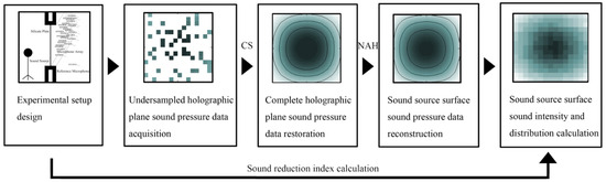
Figure 1.
Schematic diagram of the C-NAH method.
2.1. Compressed Sensing
The acoustic signal data have a local low-dimensional structure, periodicity, symmetry, etc.; so, the traditional array data must have information redundancy. The basic idea of CS theory is to compress the data during the process of data acquisition, and the original data can be restored (in order to differentiate from the NAH reconstruction of the acoustic pressure, this paper uses the term restoration to describe the acoustic reconstruction of the CS theory) with a high degree of accuracy. This idea breaks Nyquist’s theorem, and even if the sampling frequency is less than twice the analysis frequency, the original signal can be restored without aliasing, greatly simplifying the acoustic signal acquisition process.
Suppose that the acoustic signal matrix p (x, y, z1) can be sparsely represented by some orthogonal transformed basis D∈RN×N,
where P(z1)∈RN×1 is the sparse coefficient. The number k of non-zero coefficients in the sparse coefficient P(z1) varies under different transformation bases. Randomly sampling part of the data in the holographic surface to form the observation matrix H, the randomly sampled holographic surface data pcs (x, y, z) can be expressed as
The process of reducing the original data can be viewed as finding a regularized solution to the above equation under the constraint of the L0-paradigm:
The L0-paradigm problem is a nonconvex optimization problem, the solution to which requires exhaustive enumeration and is extremely complex to compute. It has been pointed out [9] that when a sparse solution exists for the (P0) problem, the corresponding (P1) problem has the same solution, in which case the above equation is equivalent to
The actual acquired signal contains noise; so, it can be assumed that
where σ denotes the noise level, and z represents the standard Gaussian white noise. Under this condition, Equation (5) will be converted to
which is the solution to the following equation:
This Lasso problem, represented by Equation (7), is equivalent to the constrained form of BPDN [34]. The first term is the data fidelity term, which quantifies the error between the reconstructed measurements and the original observed data. Minimizing this term ensures the reconstructed signal closely matches the actual measurements. The second term serves as a regularization term, promoting sparsity in the solution vector P(z1). The parameter λ > 0 is a regularization parameter that controls the trade-off between the data fidelity and the sparsity of the solution. A larger value of λ imposes a heavier penalty on the L1-norm, leading to a sparser reconstructed vector P(z1). Conversely, a smaller λ prioritizes a closer fit to the original measurements, potentially at the cost of reduced sparsity. A detailed solution of Equation (7) is given in study [29]. At this point the choice of λ is related to the dimension M of matrix P(z1) and follows the following principle:
As shown in Equation (7), the core of the compressed sensing reconstruction is to solve the L1-norm minimization problem. Finding an analytical solution for this is computationally prohibitive, especially for large datasets. Therefore, we utilize an efficient iterative algorithm, the SPGL1 [29] (Spectral Projected Gradient for L1 minimization), to find the optimal sparse solution. Its fundamental principle of L1-norm minimization is designed to recover the sparse signal while simultaneously acting as a powerful denoising algorithm. By promoting sparsity, the algorithm naturally suppresses small-amplitude components, which are often attributed to environmental noise. This inherent denoising capability significantly enhances the accuracy of the reconstructed sound field and makes the entire method highly robust to noisy measurement data. A convergence criterion based on the residual norm is utilized to determine when the iterative solving algorithm should terminate, ensuring an optimal balance between reconstruction fidelity and noise suppression:
where ε = 10−6, which is the convergence threshold.
2.2. NAH Combined with CS
The NAH is derived from the Kirchoff–Helmholtz equation:
where is the Green’s function of the field point r with respect to the point rs on the surface S. The physical significance of this equation is that the sound pressure distribution on the boundary surface S and its derivative with respect to the normal direction n can be utilized to determine the sound pressure distribution within the passive sound field V. When the surface S is assumed to consist of an infinite source plane combined with an infinite hemisphere satisfying the Sommerfield condition, and a specific Green’s function is chosen such that integral to a value of zero, Equation (9) can be further simplified to
where P(z1), P(z0) are the angular spectral expressions for the complex sound pressure distribution in the holographic plane and the source plane, P = Dp. Gd is the two-dimensional spatial Fourier transform of the corresponding Green’s function. Equation (11) establishes the relationship between the sound pressure distribution in the source plane and the sound pressure distribution in any of the parallel planes in the radiated sound field.
By combining Equations (2) and (11), the reconstructed surface sound pressure p(z0) can be obtained from sparse measurements pcs. This reconstruction is performed under the known conditions of sampling positions H, sparse transformation matrix D, and Green’s function G.
The distribution of surface normal active sound intensity I can be obtained from the product of sound pressure and normal vibration velocity:
where ρ is the medium density, ω is the angular frequency, is the wavenumber domain expression of the normal vibration velocity field, is the spatial domain expression of the normal vibration velocity field, the superscript ∗ denotes the complex conjugate, and Re denotes taking the real part. According to the ISO standard for measuring the sound insulation of a building element using the sound intensity [35], the sound reduction index RI is calculated using the following formula:
where Lp1 is the average sound pressure level in the source room, LIn is the average sound intensity level over the measurement surface in the receiving room; Sm is the total area of the measurement surface, and Sa is the area of the test specimen under test part of the area common to both the source and receiving rooms.
3. Simulation Methodology
We assume that there is a 1 m × 1 m simply supported steel plate with a thickness of 0.005 m surrounded by an infinite rigid baffle. The Young’s modulus of the steel plate is 2.1 × 10¹¹ Pa, the Poisson’s ratio is 0.28, and the density is 7.85 × 10³ kg/m3. Its first-order natural frequency is approximately 24.4 Hz. A force of 1 N is continuously excited at the center of the plate, causing the plate to emit an acoustic signal into the positive semi-infinite space. The acoustic field is recorded at 50 mm and 5 mm above the plate using a 16 × 16 sound pressure probe with an aperture exactly equal to the area of the plate. The effect of different sampling rate (SR) or signal-to-noise ratio (SNR) on the reconstruction results is analyzed from 100 Hz to 5000 Hz 1/3 octave. The numerical simulation is based on the Matlab 2020b platform (Version R2020b, MathWorks, Natick, MA, USA). In this study, the normalized mean squared error (NMSE) is used to illustrate the effectiveness of the algorithm.
where pr represents the sound pressure value reconstructed by the method proposed in this study, and ps represents the actual sound pressure value emitted from the sound source surface.
3.1. Reconstruction Under Varied Sampling Rates
The errors of the C-NAH and NAH reconstruction of surface sound pressure under different SR conditions are demonstrated in Figure 2. Since the quality of C-NAH reconstruction is related to the distribution of sampling points, 20 sets of randomly sampled images were generated consecutively, and the mean variance and distribution of the reconstruction errors are shown in the colored part of the figure. To facilitate comparison with the NAH reconstructed images, the error of the NAH reconstructed surface sound pressure is depicted in the figure using a broken line. When the SR is 10%, 20%, 30%, and 40%, the reconstruction errors of the C-NAH in the analyzed frequency range are 64.04%, 57.26%, 53.49%, and 51.55%, respectively. When fully sampled, the reconstruction error is 49.05%. It can be found that as the SR rises, the C-NAH reconstruction error gradually approaches the NAH; in fact, when the SR reaches 30%, the C-NAH reconstruction error within the analyzed frequency range is basically close to the NAH, the reconstruction effect of the middle and low frequencies is quite high, and the main error occurs in the high frequency range (above 2500 Hz). It can be found that as the SR increases, the range of the C-NAH error distribution becomes centralized, and the standard deviation gradually decreases, which indicates that the design of the mask is important only under the condition of very low SR, and that when the SR is above 20%, any mask can meet the needs of sound insulation measurements, which greatly relaxes the limitations of the method.
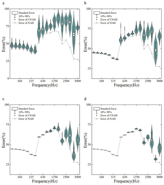
Figure 2.
Reconstruction error of C-NAH and NAH vs. SR ((a): 10%, (b): 20%, (c): 30%, (d): 40%).
Figure 3 illustrates the reconstruction results for different SRs at 200/1000/4000 Hz. Even if 40% of the sampling points are sampled for the original image, the holographic surface sound pressure distribution characteristics cannot be visualized. Although the reconstructed image using the reduced data loses some details, the CS method is used to not only approximate the original data but also to maintain a very high degree of similarity with the theoretical values. At 200 Hz, the reconstructed image is basically the same as the theoretical image. At 1000 Hz, the details at the edges of the reconstructed image are missing, and the overall magnitude is low. At 4000 Hz, the four hotspots in the center of the picture are clearly visible, and the overall contour can be roughly distinguished, although more details are lost.
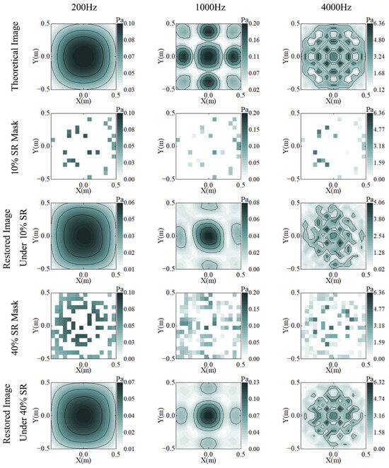
Figure 3.
Theory (row 1) and reconstruction results of C-NAH under 20% (rows 2 and 3) and 40% (rows 4 and 5) SR, at 200 (column 1), 1000 (column 2), and 4000 (column 3) Hz.
As analyzed above, the increase in SR has an important impact on the reconstruction quality, especially for complex images, which may be related to the sparseness of the image, and the application of CS theory in acoustic isolation measurements to achieve successful data restoration is inextricably linked to the characteristics of the acoustic signal. Acoustic signals are sparse. The sparsity of a signal describes the distribution of the signal energy over a certain domain, and when the signal has fewer non-zero coefficients in some orthogonal transformed basis, its sparsity is stronger. Suppose that the acoustic signal p (x,y,z) can be sparsely represented by some orthogonal transformation basis D∈RN×N In NAH theory, the most common sparse transform basis is the two-dimensional discrete Fourier transform. Through this transformation, the acoustic field representation shifts from spatial coordinates to the wavenumber spectrum. Although in the strict sense, there are components in each wave number after the transform, the acoustic array signal naturally meets the sparsity requirement of CS because the swift wave component in the acoustic wave accounts for a very small percentage and should be ignored in the acoustic isolation measurements [37]. The sparsity requirement of CS is therefore naturally satisfied by the acoustic array signal. However, as the frequency increases, the swift wave component will increase, making the signal sparsity decrease.
3.2. Reconstruction Under Varied Noise Levels
The errors of the C-NAH and NAH reconstruction of surface sound pressure under different background noise conditions are demonstrated in Figure 4. When the SNR is set to no noise, 20 dB, 10 dB, and 0 dB, the reconstruction errors in the analyzed frequency range are 57.26%, 58.67%, 60.92%, and 67.02% for C-NAH and 49.05%, 49.07%, 49.23%, and 50.31% for NAH, respectively. As the SNR decreases, the reconstruction error of C-NAH gradually increases, while the reconstruction error of NAH remains within a stable range. This indicates that the NAH has a strong robustness to noise, whereas the C-NAH is more dependent on the accuracy of the sampled data, and excessive noise interference is not allowed. The growth of the error is not linearly correlated with the decrease in the SNR, when the SNR is above 10 dB, the change in the error is relatively smooth; however, when the SNR is lower than 10 dB, the error increasingly accelerates, and the range of the distribution of the C-NAH error as well as the standard deviation increases significantly.
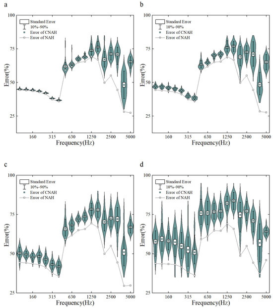
Figure 4.
Reconstruction error vs. SNR ((a): no noise, (b): 20 dB, (c): 10 dB, (d): 0 dB).
Figure 5 shows the reconstruction effect of different amounts of background noise at 20% SR. The background noise has an interfering effect on all frequency bands. At 200 Hz, the reconstructed image is no longer smooth due to the influence of the noise. At 1000 Hz, the reconstructed image is missing details at the edges, and the overall amplitude is low. At 4000 Hz, although more details are lost, the four hot spots in the center of the image can still be distinguished. This shows that the algorithm has a certain anti-interference ability.
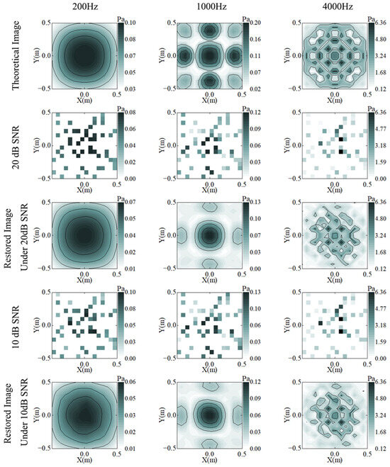
Figure 5.
Theory (row 1) and reconstruction results of C-NAH under 20 dB (rows 2 and 3) and 10 dB (row 4 and 5) SNR, at 200 (column 1), 1000 (column 2), and 4000 (column 3) Hz.
To quantitatively evaluate the effectiveness of the inherent denoising mechanism in the L1-norm minimization algorithm, we compared the reconstruction errors across the entire analyzed frequency range under two scenarios: with the denoising effect enabled and without it. As shown in Figure 6, when the denoising feature (obtained from solving the minimization problem using the SPGL1 algorithm) is activated, the reconstruction errors are lower across all frequency bands. Specifically, compared with the non-denoised case, the average error of the denoised results is reduced by approximately 3%, and this improvement is consistent across all frequency bands. This result confirms that the inherent sparsity-promoting constraint in the SPGL1 algorithm can effectively suppress measurement noise, thereby enhancing the overall reconstruction accuracy and robustness of the C-NAH method.
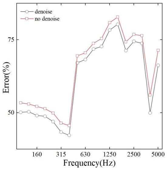
Figure 6.
Reconstruction results of denoised and non-denoised.
3.3. Influence of Mask
In Figure 2 and Figure 4, the C-NAH reconstruction errors are distributed within a certain range. This is due to the fact that the goodness of the reconstruction results is strongly related to the correlation between the observation matrix and the dictionary, and the weaker the correlation, the better its reconstruction. The matrix G = DTHTHD is defined, and the correlation is evaluated using a threshold mean correlation coefficient [38] of
where t is the threshold value, and gij is the element of the matrix G. The above equation represents the absolute average of the non-diagonal elements of the matrix G whose absolute value of the elements is greater than the threshold value, and this metric can make a better evaluation of the overall correlation between the observation matrix and the sparse basis. Figure 7 illustrates the relationship between the compression perception error and the threshold average correlation coefficient at 1000 Hz.
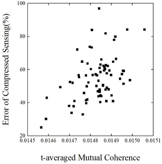
Figure 7.
T-averaged Mutual Coherence versus reconstruction error.
At a frequency of 1000 Hz, the threshold-averaged correlation coefficients of 75 randomized trials are distributed between 0.0145 and 0.0151, with a small floating range. There is a large gap in the data reduction effect, with a reconstruction error of about 25% when the coefficient is at 0.014565 and about 97% when the coefficient grows to 0.014841. Overall, the reconstruction error is positively correlated with the threshold mean correlation coefficient. Figure 7 explains well the reason for the data dispersion in the above analysis. Based on this finding, a simple observation matrix optimization strategy could be achieved by calculating the threshold average correlation coefficient of random observation matrices in large numbers and selecting observation matrices with lower correlation coefficient values to be used.
4. Experimental Data Processing
To verify the effectiveness of the proposed algorithm, two sets of experiments were conducted. The first experiment, performed in the anechoic chamber of the State Key Laboratory of Subtropical Building and Urban Science, South China University of Technology, aimed to validate the fidelity of CS in data recovery. The test platform is a 16-channel National Instruments signal acquisition instrument.(National Instruments, Austin, TX, USA) As shown in Figure 8, a 16 × 16 sound field matrix was obtained at 80 mm from the surface of a stable-emitting dodecahedron loudspeaker (Beijing Shengwang Acoustics Co., Ltd., Beijing, China) by scanning a linear array of 16 microphones (50 mm element spacing) 16 times with a 50 mm step size. All equipment was positioned more than 1.5 m from the walls to minimize reflection interference. Subsequently, 128 sampling points (a 50% sampling rate) were randomly selected from the complete matrix for data recovery, and the image restoration quality and error were evaluated.
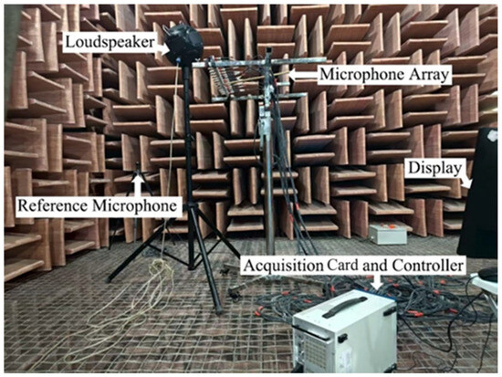
Figure 8.
Anechoic chamber experimental setup.
The second experiment was conducted in the reverberation chamber of the State Key Laboratory of Subtropical Building and Urban Science, South China University of Technology, to verify the accuracy of the proposed C-NAH theory in a field-simulated environment. The receiving room is 4.8 m long, 7.6 m wide, and 4.0 m high. The reverberation time in the mid-frequency (500 Hz) is 2.6 s. As shown in Figure 9, the test object was a double-layer 10 mm silicate plate with an area of approximately 11.7 m2. It is assembled by joining multiple smaller boards together. Most of the gaps are sealed with sealant, while the gap indicated by the arrow is not fully filled with sealant—this is intended to artificially create an acoustic defect. The same array was used, but the acquisition matrix was expanded to 32 × 32. By performing 32 scans on the left and right sides of the component (with a 50 mm step size), sound field data at 5 mm and 50 mm from the surface were recorded. To simulate a real noise environment, steady-state noise was introduced, resulting in a measured signal-to-noise ratio of 6.65 dB. Reconstruction of the normal sound intensity was performed using both the traditional NAH and the proposed C-NAH method. For the former, the complete sound pressure matrix at 50 mm was utilized. For the latter, a randomly sampled subset of this data, at a 50% sampling rate, was employed. The measured sound pressure at 5 mm from the component’s surface was converted into normal sound intensity to serve as the theoretical true value, against which the reconstruction results and errors were compared. As a key practical metric, the component’s sound reduction index was also calculated using Equations (13) to (15), based on the results from both reconstruction methods. The calculated sound reduction index was then compared with that measured by the sound pressure method [36]:
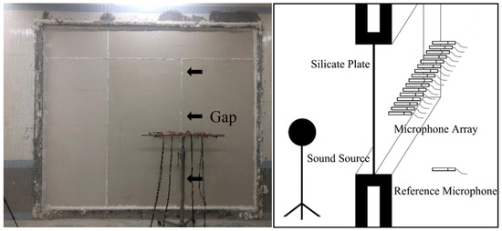
Figure 9.
Reverberation room experimental setup and schematic diagram.
Lp1 and Lp2 are the sound pressure levels of the source room and the receiving room, respectively. T is the reverberation time of the receiving room, with T0 = 0.5 s.
The holographic measurement errors and sound field reconstruction errors caused by the microphone array mismatch will have an adverse impact on the sound insulation measurement using the NAH method. Therefore, before holographic measurement, strict calibration of the amplitude and phase consistency between each channel of the microphone array is required. In this paper, under the free-field environment of a fully anechoic chamber, the transfer function method33 is adopted, with the GRAS 46AE standard microphone as the reference channel, to calibrate the frequency response characteristics of each channel of the linear array (together with its channel circuit) one by one, and thus, the frequency response characteristic correction matrix of the entire measurement system is obtained.
4.1. Anechoic Chamber Experiment
Figure 10 presents the complete sound pressure level matrix of the holographic surface (Rows 1 and 3) and the sound pressure level matrix reconstructed by the algorithm at a 50% sampling rate (Rows 2 and 4). Through comparison, the reconstructed images show a high degree of similarity to the original images in terms of overall distribution. The distribution patterns of high-value and low-value regions of sound pressure levels are basically consistent, and the shape and position of the main sound source are accurately reproduced in the reconstructed images. This indicates that the algorithm can still effectively capture the key spatial characteristics of the sound field even when the amount of data is reduced by half. In addition, the calculation and comparison of the average sound pressure level Lp2 of the matrices at the same frequency show that the two values are close, with the maximum sound pressure level error within 1 dB. The Lp2 error only increases to 2.5 dB at high frequencies (above 4000 Hz). This confirms that the reconstruction algorithm not only ensures the similarity of spatial distribution but also maintains the accuracy of the sound field energy information. The algorithm has shown excellent performance under sparse sampling conditions, successfully achieving high-fidelity sound field reconstruction. The reconstructed sound pressure level matrix is highly consistent with the original data in both spatial distribution and average energy, which strongly proves that the algorithm can maintain the accuracy of acoustic holographic imaging while significantly reducing the cost and time of data acquisition.
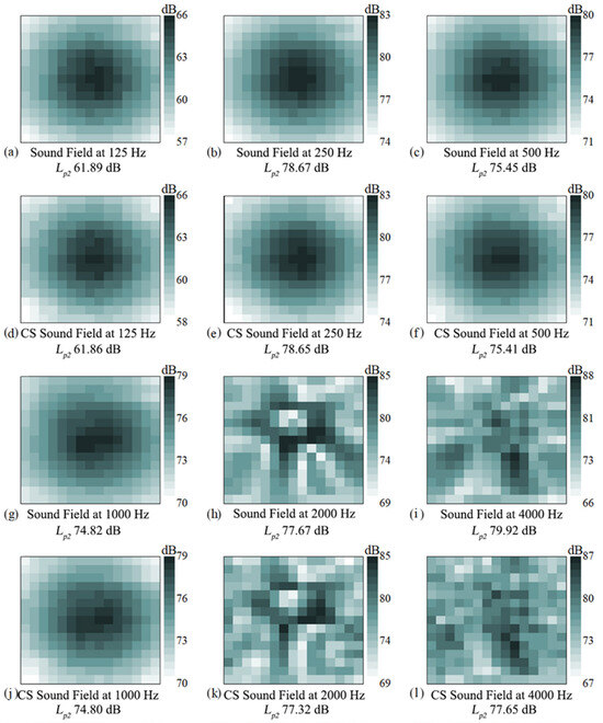
Figure 10.
Measured holographic sound pressure data (rows 1 and 3) and CS restored holographic sound pressure data (rows 2 and 4).
4.2. Reverberation Room Experiment
In order to observe more intuitively the powerful image restoration capability of C-NAH theory, the measured holographic surface data and the restoration data at 50% SR are shown in Figure 11. In Figure 11, rows 1 and 3 show the sound intensity of the nearfield sound source surface reconstructed by NAH (full sampling). Observation of the image shows that the 18th column of the measured data is significantly larger, creating an acoustic defect. Observation of the surface of the component reveals that there is a splicing seam, and the acoustic defect is most likely caused by the poor splicing of the two components. The defect is observed in all frequency bands. Rows 2 and 4 show the reduced data at 50% SR. Similarly, the 18th column of data in the holographic surface data after CS processing is large, and the image shows a similar structure to the measured data, indicating that the C-NAH theory can achieve super-resolution image restoration. At the analyzed frequency, the image restoration error is about 44.94%. There are some differences between the restored image and the measured data of the holographic surface, such as the low intensity of the upper part of the 18th column of data, which is caused by the distribution of the observation matrix. However, the calculated normal sound intensity levels show that the C-NAH exhibits values almost identical to those of the NAH, with an error within 2 dB.
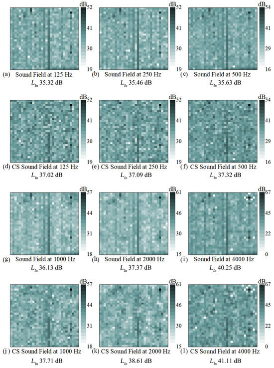
Figure 11.
The sound intensity level of nearfield sound source surface reconstructed by NAH (rows 1 and 3) and C-NAH (rows 2 and 4).
Figure 12 shows the results of reconstructing the two sets of data using the same NAH method and comparing them with the measured data at 5 mm. The average reconstruction error of the NAH method is 93.72%, while the reconstruction error of the C-NAH method is 98.53%. Both methods showed a consistent trend of smaller errors in the lower frequency range and larger errors in the higher frequency range. When the analyzed frequency rises above 2000 Hz, the reconstruction error increases significantly, which is contrary to the simulation conclusions and can be believed to be due to the measurement error at high frequencies. Comparing the errors of the two methods, the reconstruction error enhancement at full frequency is about 4.81%, the error is smaller in the low frequency range and larger in the high frequency range, and the CS theory makes the reconstruction error enhancement of 15.11% at the frequency of 5000 Hz. The CS restoration process does not depend on the accuracy of the numerical measurements, and therefore, this conclusion is consistent with the simulation results.
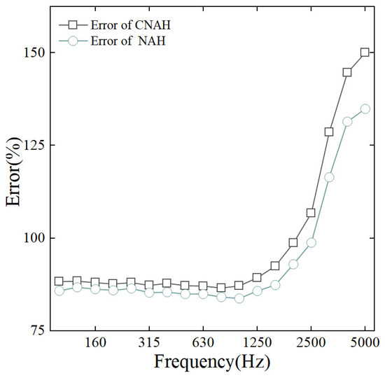
Figure 12.
Reconstruction error of NAH and C-NAH.
Finally, the component sound reduction index measured by different methods shows a high degree of consistency. The sound reduction index DnT measured by the sound pressure method is 59 dB, the sound reduction index RI measured by the NAH is 60 dB, and the sound reduction index RI measured by the C-NAH is 58 dB. The error is controlled within 1 dB, which indicates that the C-NAH method has a high degree of accuracy.
5. Discussion
Our findings demonstrate that the proposed C-NAH method successfully enables high-fidelity sound field reconstruction and sound insulation evaluation with a significantly reduced data sampling rate. This represents a novel approach to addressing the efficiency challenges of traditional acoustic measurements. The results show that the sparsified measurement points maintain high original data restoration accuracy, with the negligible error between the reduced and original data not compromising subsequent sound field reconstruction and sound insulation measurements. Based on the research results of this paper, the downsampling sound insulation measurement technique combined with compressed perception is a sound insulation measurement technique with high sampling efficiency and low data volume. Due to its non-orthogonal sampling characteristics, it can not only adapt to the conventional building acoustic insulation defect detection scenarios but also adapt to the scenarios where there is a certain amount of steady-state noise interference and shaped walls. Moreover, theoretically analyzed, this method can also be expanded to the field of sound intensity method sound insulation measurement.
In the experimental results of this paper, the middle and low frequency errors are basically stabilized at 80%, which is basically consistent with previous studies [15]. However, the error rises rapidly above 2500 Hz, resulting in a higher overall error. Regarding the reason for the high reconstruction error of the simulation results as well as the measured data in the paper, it can be believed that it is due to the NAH algorithm. On the one hand, since the spacing of the microphone array is 50 mm, which is close to half of the wavelength of a 2500 Hz sound wave (approximately 68 mm), a spatial aliasing effect will occur in this case. On the other hand, since the holographic aperture is much smaller than the specimen size, the leakage generated by truncating the data at the aperture edges is more obvious, consistent with Xiong’s findings [39]. The trend of the high-frequency part of the measured results is somewhat different from that of the simulation results, which may be due to the operational error in the measurement, in addition to the fact that the algorithm has a larger error in the high-frequency case. Comparing the C-NAH and NAH reconstruction errors, it can be found that there is only a 4.81% improvement in the full frequency range, which is consistent with the simulation results, indicating that using the CS method does not lose too much information about the sound field while drastically reducing the number of sampling points. The component sound reduction index exhibits agreement, with deviations tightly constrained within a 1 dB range. This close correlation between different measurement approaches not only validates the robustness of the techniques but also highlights their precision in sound insulation evaluation, with variations well within acceptable engineering tolerances for acoustic measurements. The minimal discrepancy observed substantiates the C-NAH’s capability to deliver consistent results comparable to established techniques while maintaining measurement integrity. These findings strongly support the adoption of this methodology for high-precision acoustic assessments where reliable and reproducible results are paramount. Besides enhancing efficiency, the C-NAH method offers another notable advantage over other novel resolution-boosting algorithms [40,41,42]: it functions as a data pre-processing technique independent of specific reconstruction algorithms. This versatility allows the proposed method to be broadly compatible with various acoustic holography techniques, such as SONAH and BEM.
While the C-NAH method enables maximizing the direct sound signal by measuring close to the source, the influence of the reverberation time remains a critical factor that warrants systematic evaluation. In the reverberation chamber, the calculated mid-frequency (500 Hz) reverberation radius is approximately 0.25 m. By definition [43], when the measurement distance is significantly smaller than this radius, the energy of the direct sound is expected to be substantially higher than that of the reverberant sound. Given our measurement distance of only 0.05 m, the SNR is estimated to be over 14.0 dB based on the inverse square law. This suggests that nearfield measurements can achieve a high SNR even in highly reverberant environments. This theoretical finding is consistent with our experimental results from the SNR analysis in Section 3.2. Under low SNR conditions of 10 dB and 0 dB, the reconstruction errors increased by only 3.66% and 9.76%, respectively, demonstrating the method’s strong robustness against reverberant noise. Furthermore, the existing literature [39] has experimentally confirmed that the impact of reverberation time on sound pressure levels and reconstructed sound intensity is negligible under similar conditions (a distance of 0.04 m and reverberation time up to 3.4 s). In conclusion, a combination of theoretical analysis and empirical evidence confirms that the C-NAH method is effective in addressing the challenges posed by conventional reverberant environments.
Although C-NAH has demonstrated strong data downsampling capability, the approach is not without its limitations, and further research is warranted. First, the algorithms mentioned in this paper are essentially operations on one-dimensional signals; so, the two-dimensional structure of the image is bound to be neglected when dealing with the image problem. Fang et al. [44] propose an approximate observation sparse SAR imaging model, which is able to retain a certain amount of two-dimensional image structure. Analyzing the difference between the one-dimensional algorithm and the two-dimensional algorithm may help to achieve more accurate image restoration. Second, analyzing the results of this paper, the effect of the noise reduction algorithm is limited, and how to improve the robustness of CS is an issue worth studying. Finally, since the method is only used as a pre-processing means for nearfield acoustic holography acoustic isolation measurement technology, the reconstruction effect is largely dependent on the selected NAH method, and scholars have already verified the validity of applying the CS theory in ESM, SONAH, and other algorithms [16,17,18,19,20,21,22,23,24,25]. However, whether the CS theory can be compatible with ESM and SONAH et al. in acoustic isolation measurements remains a worthwhile exploratory topic.
6. Conclusions
In this study, based on the redundancy characteristics of acoustic signals, a compressed perception method is applied to compress and perceive the signals simultaneously, and the acoustic isolation measurement method is investigated. The main contributions of this paper are as follows:
- Introduce the theory of compression perception in sound insulation testing to realize higher accuracy surface sound pressure reconstruction as well as sound insulation measurement at sampling points below Nyquist’s theorem.
- Consider a noise-adapted basis pursuit algorithm to realize the robustness of reconstruction results in noisy environments.
- Provide and analyze a more stable observation matrix design strategy to reduce the error in sound insulation calculation.
Limited by the Nyquist theorem, the traditional acoustic measurement method has to collect a large amount of data in order to obtain accurate acoustic signal data on the surface of the component, which is a waste of human and material resources as it requires high requirements on hardware equipment and operators. The proposed method addresses this challenge by achieving acoustic imaging at sub-Nyquist. According to the simulation results of this paper, under the condition of no noise interference, C-NAH only needs 30% SR to restore the complete holographic surface sound pressure data, which can accurately reflect the radiated acoustic characteristics of the component, and its reconstruction error is as low as 53.49%. Compared with the reconstruction error under the complete sampling condition, it is only 4.44% higher. The anechoic room experiment verified that conclusion. Although the algorithm can resist noise interference to a certain extent, it is still not applicable to the conditions of lower SNR, and a SNR of 10 dB or more is a more suitable interval. The reverberation room experiment basically verified the above conclusion. The experiment proves that under the conditions of 50% sampling points and 6.65 dB SNR, the C-NAH method can locate the sound insulation defects of building components more accurately, and compared with NAH, the surface sound pressure reconstruction error is only increased by 8.21%, and the error of the measured sound reduction index is within 1 dB. The findings of this paper provide strong theoretical and practical support for the development of high-efficiency low-cost acoustic inspection technology for the built environment.
Author Contributions
Conceptualization, C.Y. and H.W.; methodology, C.Y. and Q.W.; software, C.Y. and S.L.; validation, C.Y.; formal analysis, C.Y. and Q.W.; investigation, C.Y. and S.L.; data curation, C.Y.; writing—original draft preparation, C.Y. and Q.W.; writing—review and editing, H.W.; supervision, H.W.; funding acquisition, H.W. All authors have read and agreed to the published version of the manuscript.
Funding
This research was funded by National Natural Science Foundation of China, grant number [52078218].
Data Availability Statement
The original contributions presented in this study have been open-sourced and can be accessed at https://github.com/ChenxiYang188/C-NAH-Data (accessed on 27 October 2025). Further inquiries can be directed to the corresponding author.
Conflicts of Interest
The authors declare no conflicts of interest.
Abbreviations
The following abbreviations are used in this manuscript:
| NAH | Nearfield acoustic holographic |
| CS | Compressed sensing |
| C-NAH | Compressed nearfield acoustic holographic |
| SR | Sample rate |
| SAR | Synthetic aperture radar |
References
- Maynard, J.D.; Williams, E.G.; Lee, Y. Nearfield acoustic holography: I. Theory of generalized holography and the development of NAH. J. Acoust. Soc. Am. 1985, 78, 1395–1413. [Google Scholar] [CrossRef]
- Wu, H.; Zhang, N.; Zha, Y.; Gao, J.; Zhou, H.; Jiang, W. A hybrid nearfield acoustic holography based on the mapping relationship and boundary element method. Appl. Acoust. 2024, 216, 109823. [Google Scholar] [CrossRef]
- Wu, W.Y.; Zhang, X.Z.; Zhang, Y.B.; Bi, C.X. Real-time nearfield acoustic holography using particle velocity. J. Acoust. Soc. Am. 2024, 155, 3394–3409. [Google Scholar] [CrossRef] [PubMed]
- Wang, H.; Xiong, W.; Wang, Q.; Yang, Y.; He, B. Sound insulation measurement of building components combining diffuse acoustic field excitation and near-field acoustic holography reconstruction. Shenxue Xuebao/Acta Acust. 2023, 48, 1021–1035. [Google Scholar] [CrossRef]
- Cheng, W.; Ni, J.; Song, C.; Ahsan, M.M.; Chen, X.; Nie, Z.; Liu, Y. Conical Statistical Optimal Near-Field Acoustic Holography with Combined Regularization. Sensors 2021, 21, 7150. [Google Scholar] [CrossRef]
- Zhang, M.Y.; Hu, D.Y.; Yang, C.; Shi, W.; Liao, A.H. An improvement of the generalized discrete Fourier series based patch near-field acoustical holography. Appl. Acoust. 2021, 173, 107711. [Google Scholar] [CrossRef]
- Xie, S.H.; Ma, H.Y.; Cao, J.M.; Mo, F.S.; Cheng, Q.; Li, Y.; Hao, T. Refined acoustic holography via nonlocal metasurfaces. Sci. China Phys. Mech. Astron. 2024, 67, 239506. [Google Scholar] [CrossRef]
- Chai, K.; Lou, J.J.; Li, R.H.; Hu, J.B. Research and experiment on patch near-field acoustic holography based on two-level iteration. J. Ship Mech. 2024, 28, 1441–1450. [Google Scholar] [CrossRef]
- Donoho, D.L. Compressed sensing. IEEE Trans. Inf. Theory 2006, 52, 1289–1306. [Google Scholar] [CrossRef]
- Lustig, M.; Donoho, D.L.; Pauly, J.M. Sparse MRI: The application of compressed sensing for rapid MR imaging. Magn. Reson. Med. 2007, 58, 1182–1195. [Google Scholar] [CrossRef]
- Usman, M.; Prieto, C.; Schaeffter, T.; Botnar, R.M. K-t group sparse: A method for accelerating dynamic MRI. Magn. Reson. Med. 2011, 66, 1163–1176. [Google Scholar] [CrossRef]
- Baraniuk, R.; Steeghs, P. Compressive radar imaging. In Proceedings of the IEEE Radar Conference, Waltham, MA, USA, 17–20 April 2007; pp. 128–133. [Google Scholar] [CrossRef]
- Coker, J.D.; Tewfik, A.H. Compressed sensing and multistatic SAR. In Proceedings of the IEEE International Conference on Acoustics, Speech and Signal Processing, Taipei, Taiwan, 19–24 April 2009; pp. 1097–1100. [Google Scholar] [CrossRef]
- Stojanovic, I.; Karl, W.C. Imaging of Moving Targets with Multi-Static SAR Using an Overcomplete Dictionary. IEEE J. Sel. Top. Signal Process. 2010, 4, 164–176. [Google Scholar] [CrossRef]
- Gilles, C.; Laurent, D.; Antoine, P. Nearfield Acoustic Holography using sparsity and compressive sampling principles. J. Acoust. Soc. Am. 2012, 132, 1521–1534. [Google Scholar] [CrossRef]
- Xiao, Y.; Yuan, L.; Wang, J.; Hu, W.; Sun, R. Sparse Reconstruction of Sound Field Using Bayesian Compressive Sensing and Equivalent Source Method. Sensors 2023, 23, 5666. [Google Scholar] [CrossRef] [PubMed]
- Xiao, Y.; Yuan, L.; Liu, Y.; Wang, J.; Hu, W.; Sun, R.; Liu, Y.; Ni, P. Sparse reconstruction of sound field using pattern-coupled Bayesian compressive sensing. J. Acoust. Soc. Am. 2024, 156, 548–559. [Google Scholar] [CrossRef] [PubMed]
- Zan, M.; Xu, Z.; He, J. A block bayesian compressive sensing method based on the equivalent source method for near-field acoustic holography. J. Vib. Control 2023, 29, 1303–1314. [Google Scholar] [CrossRef]
- Hu, D.Y.; Liu, X.Y.; Xiao, Y.; Fang, Y. Fast Sparse Reconstruction of Sound Field Via Bayesian Compressive Sensing. J. Vib. Acoust. 2019, 141, 041017. [Google Scholar] [CrossRef]
- He, Y.; Chen, L.; Xu, Z.; Zhang, Z. A compressed equivalent source method based on equivalent redundant dictionary for sound field reconstruction. Appl. Sci. 2019, 9, 808. [Google Scholar] [CrossRef]
- Geng, L.; Chen, X.G.; He, C.D.; Chen, W.; He, S.P. Compressive nonstationary near-field acoustic holography for reconstructing the instantaneous sound field. Mech. Syst. Signal Process. 2023, 204, 110779. [Google Scholar] [CrossRef]
- Zheng, Y.; Zhang, F.; Xiao, Z.; Zhou, R.; Zhang, Y.; Bi, C. Multi-frequency equivalent source near-field acoustic holography method based on common sparse Bayesian learning. J. Vib. Shock 2024, 43, 260–267. [Google Scholar] [CrossRef]
- Wu, B.H.; Hsu, W.J. Application of compressive sensing to equivalent source method on near-field acoustic holography. Appl. Acoust. 2024, 223, 110075. [Google Scholar] [CrossRef]
- Chaitanya, S.K.; Srinivasan, K. Equivalent source method based near field acoustic holography using multipath orthogonal matching pursuit. Appl. Acoust. 2022, 187, 108501. [Google Scholar] [CrossRef]
- Shi, T.; Bolton, J.S.; Eberhardt, F. A hybrid compressive sensing approach to noise source visualization: Application to a diesel engine. J. Acoust. Soc. Am. 2023, 153, A55. [Google Scholar] [CrossRef]
- Topp, J.A.; Gilbert, A.C. Signal recovery from random measurements via orthogonal matching pursuit. IEEE Trans. Inf. Theory 2007, 53, 4655–4666. [Google Scholar] [CrossRef]
- Blumensath, T.; Davies, M.E. Iterative hard thresholding for compressed sensing. Appl. Comput. Harmon. Anal. 2009, 27, 265–274. [Google Scholar] [CrossRef]
- Gorodnitsky, I.F.; Rao, B.D. Sparse signal reconstruction from limited data using FOCUSS: A re-weighted minimum norm algorithm. IEEE Trans. Signal. Process. 1997, 45, 600–616. [Google Scholar] [CrossRef]
- Figueiredo, M.A.T.; Nowak, R.D.; Wright, S.J. Gradient Projection for Sparse Reconstruction: Application to Compressed Sensing and Other Inverse Problems. IEEE J. Sel. Top Signal Process. 2007, 1, 586–597. [Google Scholar] [CrossRef]
- Li, Y.; Zhao, H.; Liu, F.; Wang, G. Bayesian Compressive Sensing with Variational Inference and Wavelet Tree Structure for Solving Inverse Scattering Problems. IEEE Trans. Antennas Propag. 2024, 72, 8750–8761. [Google Scholar] [CrossRef]
- Liu, J.; Wu, Q.; Amin, M.G. Multi-Task Bayesian compressive sensing exploiting signal structures. Signal Process. 2021, 178, 107804. [Google Scholar] [CrossRef]
- Wang, R.; Bai, Y.; Yu, L.; Dong, G. Bayesian compressive sensing for identifying tonal acoustic modes of fan noise in the duct. Acta Acust. 2025, 50, 187–200. [Google Scholar] [CrossRef]
- Chen, S.; Donoho, D.L.; Saunders, M.A. Atomic decomposition by basis pursuit. SIAM Rev. 2001, 43, 129–159. [Google Scholar] [CrossRef]
- Van den Berg, E.; Friedlander, M.P. Probing the Pareto frontier for basis pursuit solutions. SIAM J. Sci. Comput. 2008, 31, 890–918. [Google Scholar] [CrossRef]
- International Standard ISO 15186-2; Acoustics—Measurement of Sound Insulation in Buildings and of Building Elements Using Sound Intensity—Part 2: Field Measurements. ISO: Geneva, Switzerland, 2003.
- International Standard ISO 16283-1; Acoustics—Field Measurement of Sound Insulation in Buildings and of Building Elements-Part 1: Airborne Sound Insulation. ISO: Geneva, Switzerland, 2014.
- Jacobsen, F.; Tiana-Roig, E. Measurement of the sound power incident on the walls of a reverberation room with near field acoustic holography. Acta. Acust. United Acust. 2010, 96, 76–81. [Google Scholar] [CrossRef]
- Chen, X.Z.; Wang, Z.P.; Liu, Z.S.; Chen, X.D. Correcting the Phase Mismatch Errors of the Acoustic Intensity Measuring System by Transfer Function Method. Yiqi Yibiao Xuebao 1994, 4, 405–409. [Google Scholar]
- Xiong, W. Research on Measurement Method of Airborne Sound Insulation of Building Components Based on Nearfield Acoustic Holography. Ph.D. Thesis, South China University of Technology, Guangzhou, China, 2022. [Google Scholar]
- Cheng, W.; Bai, Y.; He, Y. Resolution enhanced statistically optimal cylindrical near-field acoustic holography based on equivalent source method. Meas. Sci. Technol. 2022, 33, 055015. [Google Scholar] [CrossRef]
- He, H.; Li, H.; Yan, J.; Wu, S. Application of equivalent source intensity density interpolation in near-field acoustic holography. Meas. Sci. Technol. 2023, 34, 115101. [Google Scholar] [CrossRef]
- Li, Y.; Wang, J.; Li, S.; Liu, B. Sub-wavelength focusing for low-frequency sound sources using an iterative time reversal method. Meas. Sci. Technol. 2022, 33, 125402. [Google Scholar] [CrossRef]
- Kinsler, L.E.; Frey, A.R.; Coppens, A.B.; Sanders, J.V. Fundamentals of Acoustics, 4th ed.; John Wiley & Sons Inc.: Hoboken, NJ, USA, 1999. [Google Scholar]
- Fang, J.; Xu, Z.; Zhang, B.; Hong, W.; Wu, Y. Fast compressed sensing SAR imaging based on approximated observation. IEEE J. Sel. Top Appl. Earth Obs. Remote Sens. 2014, 7, 352–363. [Google Scholar] [CrossRef]


Disclaimer/Publisher’s Note: The statements, opinions and data contained in all publications are solely those of the individual author(s) and contributor(s) and not of MDPI and/or the editor(s). MDPI and/or the editor(s) disclaim responsibility for any injury to people or property resulting from any ideas, methods, instructions or products referred to in the content. |
© 2025 by the authors. Licensee MDPI, Basel, Switzerland. This article is an open access article distributed under the terms and conditions of the Creative Commons Attribution (CC BY) license (https://creativecommons.org/licenses/by/4.0/).