1. Introduction
Corrosion and pitting defects commonly develop in environments exposed to moisture, corrosive chemicals, or harsh atmospheric conditions. In industrial equipment, these defects frequently form at welds, joints, or stressed areas where protective coatings have deteriorated. Detecting such defects is essential for pipelines, storage tanks, and marine structures to maintain structural integrity, prevent failures or leaks, and mitigate costly repairs and environmental risks.
Low-frequency guided wave inspection is widely used for its ability to cover large areas from a single transducer position [
1,
2,
3,
4]. It is effective for detecting and locating damaged regions but struggles to estimate the maximum defect depth accurately. Detection near structural features, such as pipe supports or T-joints, is also challenging due to strong reflections from low-frequency waves. At higher frequencies, guided waves exhibit minimal reflection from structural features, improving sensitivity to deeper and smaller defects [
5,
6]. However, their application is complicated by the presence of multiple dispersive modes, making implementation challenging. Balasubramaniam et al. [
7] introduced the concept of higher order modes cluster (HOMC) for guided wave inspection. This method utilizes Lamb modes in the 15 to 35 MHz mm frequency–thickness range, resulting in an excited wave packet that is nearly nondispersive. As a result, HOMC offers higher spatial resolution than low-frequency guided wave methods and reduces scattering in complex geometries such as T-joints. Moreover, the HOMC approach overcomes the challenge of generating a pure wave mode. Angled wedge transducers or electromagnetic acoustic transducer (EMAT) setups can effectively excite a group of higher order modes without requiring precise tuning. In most studies, HOMC guided waves are generated using piezoelectric transducers mounted on plastic wedges. Ratnam et al. [
8] proposed an alternative method employing meander-coil EMATs for wave generation. HOMC guided waves have been successfully used to detect notch-like defects in plates at room temperature [
9,
10], and Reddy et al. [
11] extended their application to elevated temperatures up to 300 °C. These waves, whether propagating axially or circumferentially, have also been applied for pipe inspections [
12,
13]. A notable characteristic of HOMC guided waves is their low surface motion, mainly due to the dominance of the A1 mode. However, research on their effectiveness in the presence of surface features such as T-joints and coatings remains limited [
14].
Evaluating sharp, pitting-type defects is challenging due to their complex shapes and limited surface indications. HOMC guided waves, known for their long-distance propagation and sensitivity to complex defect profiles, are particularly suitable for such inspections. However, interpreting the complex interactions between HOMC guided waves and sharp defects remains a substantial challenge. Machine learning offers a promising solution by analyzing the interaction signals without heavy reliance on domain knowledge. For instance, simulations of laser-generated Rayleigh waves interacting with subsurface defects produced reliable laser-ultrasonic signals. These signals were used to train a backpropagation neural network (BPNN) to predict the width of subsurface cracks [
15]. Similarly, ultrasonic signals from sensor pairs in a pitch-catch configuration were used to calculate damage indices, which were then fed into an artificial neural network (ANN) for classification and structural condition assessment [
16]. This demonstrates the potential of machine learning for defect characterization and structural health monitoring.
This study analyzes the characterization of welded defects in T-joint structures using reflected and transmitted HOMC guided waves. In addition, sharp defects in plate-like structures are initially characterized using a fitting model based on reflection coefficients. To enhance the evaluation, a machine learning approach is developed and compared with the performance of the conventional fitting method. The rest of this paper is organized as follows:
Section 2 introduces the HOMC guided wave inspection method, the framework of the developed machine learning approach, and the finite element model setup used in this study.
Section 3 presents the key findings from the evaluation of sharp notches in T-joint and plate-like structures.
Section 4 discusses the prediction accuracy of both methods and their limitations. Finally, concluding remarks are provided in
Section 5.
2. Materials and Methods
2.1. Sensitivity of Higher Order Modes Cluster Guided Waves to Sharp Defects
Guided wave inspection is generally more effective when employing non-dispersive modes. Consequently, fundamental guided wave modes, such as S0 and SH0, are extensively utilized. To enhance sensitivity to pitting-type defects, higher frequency guided wave modes have garnered increasing attention.
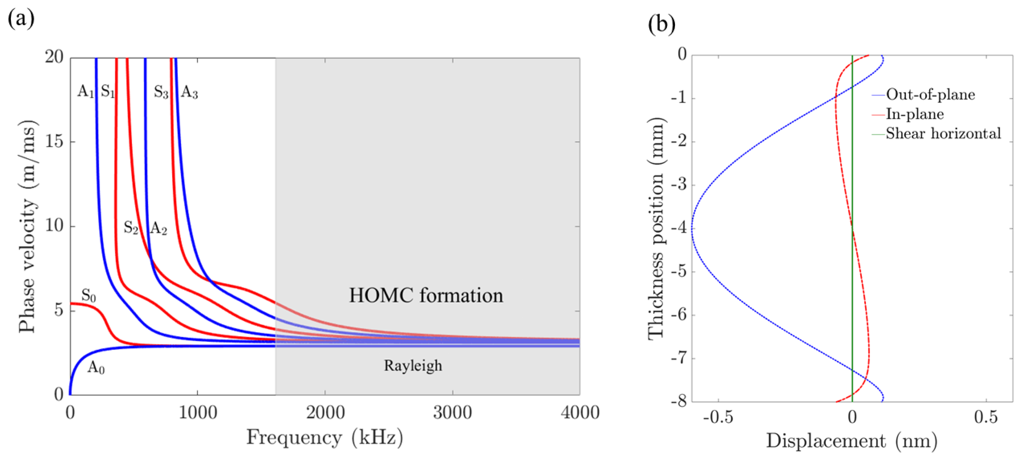
Figure 1a presents the phase velocity dispersion curves for the first eight modes of an 8 mm thick aluminum plate, generated using the Dispersion Calculator software [
17] or a SAFE-based dispersion calculator [
18]. For high-frequency–thickness products, the A0 and S0 modes asymptotically approach the Rayleigh wave velocity, while the remaining modes tend toward the bulk shear wave velocity. In the higher order modes cluster region, the wave packets exhibit nearly non-dispersive behavior, providing excellent spatial resolution. While Rayleigh waves offer completely nondispersive behavior, their substantial surface motion makes them highly sensitive to surface features such as T-joints and surface roughness. In contrast, the HOMC waves exhibit minimal surface motion, making them less sensitive to surface irregularities.
Figure 1b illustrates the deflected shape of the A1 mode, which dominates in the HOMC region. Notably, the A1 mode exhibits minimal surface motion, reducing its sensitivity to surface conditions.
The transmitted and reflected Lamb waves, as well as Rayleigh waves, have been studied and employed for the characterization of surface and subsurface defects [
19,
20]. In this study, the transmission and reflection coefficients are determined using enveloped signals. The transmission coefficient (
) is defined as the ratio of the maximum amplitude of the gated transmitted wave to that of the incident wave, while the reflection coefficient (
) is the ratio of the maximum amplitude of the gated reflected wave to that of the incident wave.
2.2. Finite Element Model Setup
Finite element analysis was performed to study the wave behavior of HOMC on non-planar structures like T-joints. It was also used to evaluate their sensitivity in detecting sharp and deep defects in plate-like structures. For optimal wave excitation, a 1-inch transducer mounted on a 62° PMMA wedge was utilized. The selection of the transducer size and wedge angle was guided by considerations of the wavenumber bandwidth reduction due to the increased projected excitation length, as well as the sensitivity of modal excitation to variations in the wedge angle [
14]. The excitation signal consisted of a 5-cycle Hanning-windowed toneburst with a center frequency of 2.25 MHz. A surface line scan was simulated to facilitate either 2D FFT analysis or enhance the received HOMC wave packets. Finite element simulations were conducted using the ABAQUS/CAE software package in a 2D plane strain configuration. The FE model utilized CPS4R elements, with a time step of 2 ns and an element size of 0.1 mm to ensure numerical stability and accuracy.
Figure 2 shows the simulation setup for a T-joint structure. It consists of an 8 mm thick horizontal aluminum plate rigidly connected to a similar 8 mm thick vertical plate. The plates have the typical properties of aluminum (e.g., density
, Young’s modulus
, Poisson’s ratio
). Wave excitation was achieved using a wedge transducer positioned on the upper surface. The defect was modeled as a notch at the joint base. To reduce the influence of Rayleigh waves on the received signals, a 50 mm long monitoring region was placed on the lower surface of the structure with monitoring points spaced at 0.5 mm intervals. The monitoring line positioned before the joint was used to calculate the reflection coefficient, while the monitoring line located after the joint was used to determine the transmission coefficient.
To streamline the generation of a batch of FE models for machine learning studies, the wave transduction process was simulated using phased excitation. This method applied time delays calculated based on the time-of-flight of the longitudinal wave propagating through the angled wedge.
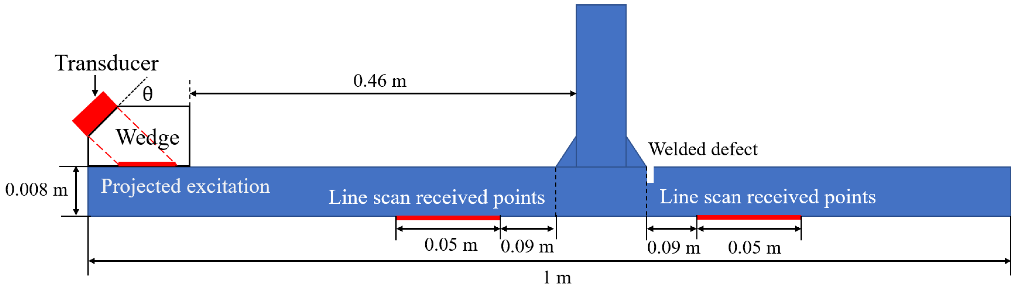
Figure 3 presents the complete FE setup for an 8 mm thick aluminum plate, where the wedge transducer was modeled using out-of-plane line excitations with integrated time delays. The excitation source was positioned 0.425 m away from the scan line. The defect has two different widths, with one measuring 1 mm, which exceeds one wavelength, and the other measuring 0.5 mm, which is smaller than one wavelength. The defect thickness varies up to 4 mm, representing 50% of the 8 mm plate thickness. The effects of the total length of the phased excitation, the number of line excitation sources, and the spacing between individual line sources on the signal-to-noise ratio (SNR) of the desired wave modes were analyzed using 2D FFT. Detailed results are presented in
Section 3.2. To prevent energy leakage and reflections from re-entering the plate structure, Absorbing Layers using Increasing Damping (ALID) elements [
21] were implemented adjacent to the acoustic element layer. Two line scans, comprising multiple monitoring points, were positioned on opposite surfaces of the plate. The line scan on the upper surface was utilized to calculate the reflection coefficient, while the line scan on the lower surface was employed to calculate both the reflection coefficient and perform 2D FFT analysis.
2.3. Machine Learning Approach for Sharp Defects Characterization
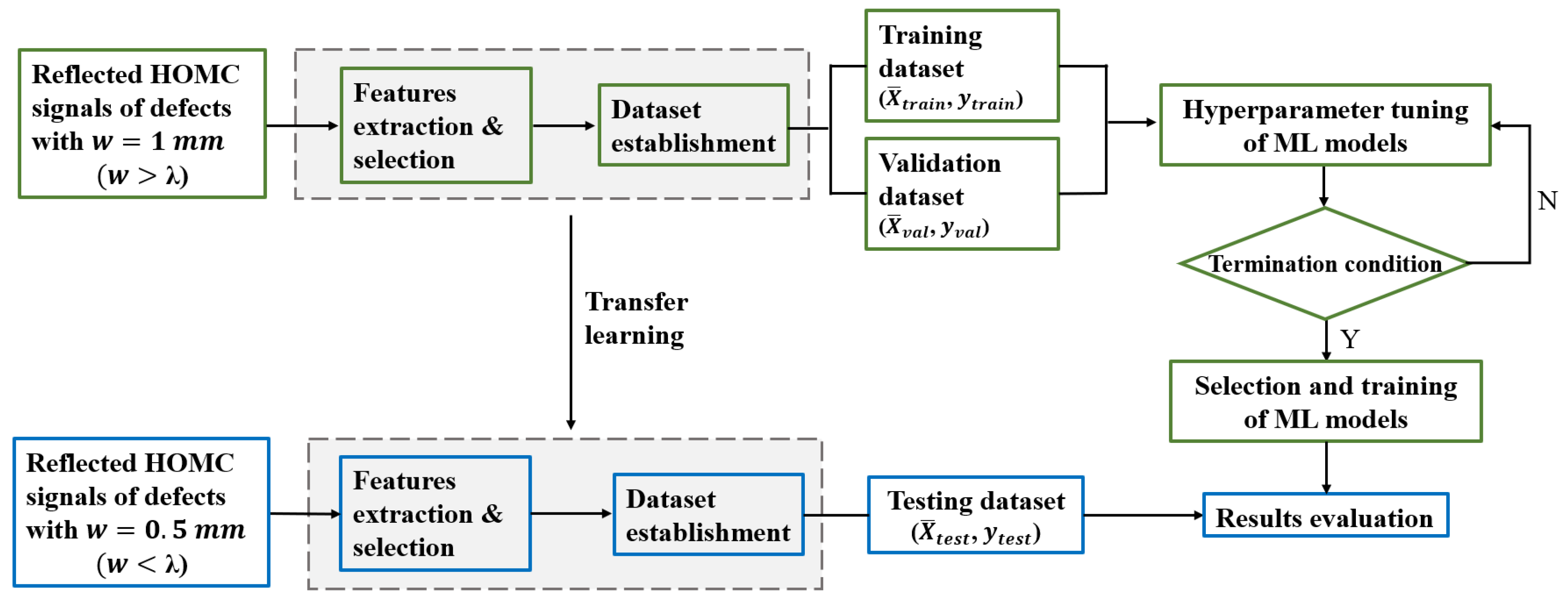
The flowchart of the proposed ML method is presented in
Figure 4. In the initial stage, a total of 19 features were extracted from the reflected wave signals, comprising 11 time-domain features, 4 frequency-domain features, and 4 wavelet transform features. Subsequently, principal component analysis (PCA) [
22] was employed to investigate the interdependencies among these features and to perform dimensionality reduction on the feature space. This step identified the most significant features relevant to the dataset. To enhance generalization across datasets, transfer learning was employed to align the feature spaces of the training and testing datasets. Specifically, domain adaptation techniques were utilized to ensure compatibility between
and
. A straightforward approach involved standardizing and aligning the distributions of the datasets explicitly. Next, the training and validation datasets were used for training and hyperparameter tuning of the ML models. The optimized ML models were deployed to predict the depths of defects with a width of 0.5 mm, smaller than one wavelength. The training and validation data, however, were based on defects with a width of 1 mm, larger than one wavelength.
Five widely used machine learning models were chosen to predict pitting depths: Random Forest (RF), Gradient Boosting (GB), Support Vector Machine (SVM), K-Nearest Neighbors (KNN), and Multilayer Perceptron (MLP). Random Forest is an ensemble learning method that enhances predictive performance by aggregating the outputs of multiple decision trees (DTs). The final prediction of the RF is obtained by averaging the outputs of these individual trees. RF has been shown to outperform single DTs in many practical applications. Similarly, the Gradient Boosting algorithm leverages multiple DTs to achieve improved performance. Unlike RF, where DTs are trained independently, GB trains DTs sequentially in a stagewise manner, with each tree correcting the errors of its predecessors. Support Vector Machine is designed to identify a hyperplane that maximizes the margin between data groups, enabling effective separation. For nonlinear regression tasks, SVM employs a kernel function to map the data from its original feature space to a higher-dimensional space, where linear separation becomes feasible. This capability makes SVM particularly effective in high-dimensional settings, such as when the number of features exceeds the number of samples. However, SVM does not inherently provide probabilistic predictions, and proper regularization is necessary to minimize the risk of overfitting. The K-Nearest Neighbors algorithm makes predictions for a given data point based on the proximity of its neighbors in the feature space. KNN is highly flexible, easily adapting to new data, and requires minimal hyperparameter tuning. However, it is memory-intensive and demands significant data storage. In addition, KNN is susceptible to overfitting, particularly in high-dimensional spaces, due to the curse of dimensionality. The Multilayer Perceptron is a type of artificial neural network composed of multiple layers of interconnected neurons. It is particularly effective for modeling complex nonlinear relationships between inputs and outputs. MLP employs backpropagation for training, adjusting the weights of its connections to minimize prediction errors. With its ability to learn intricate patterns, MLP is suitable for a wide range of tasks, including regression and classification. However, MLP often requires careful tuning of hyperparameters, such as the number of layers, neurons per layer, and learning rate, to achieve optimal performance. In addition, it can be computationally expensive and prone to overfitting if not regularized properly. The machine learning models were developed and validated using Python 3.7.
To enhance the performance of the machine learning algorithms, the hyperparameters for each model were optimized using the current dataset. Random search [
23] was employed as an efficient and practical method for hyperparameter tuning, particularly suited to high-dimensional search spaces. Unlike grid search, which systematically evaluates all possible combinations, random search samples hyperparameters randomly, enabling the discovery of effective configurations with a significantly lower computational cost. This method is especially beneficial when only a subset of hyperparameters has a substantial impact on model performance, as it avoids excessive evaluations of less influential parameters. Moreover, random search supports the flexible exploration of continuous or non-uniform distributions, increasing the likelihood of identifying optimal configurations.
3. Results
3.1. Inspection of T-Joints
Inspection of corrosion in regions beyond visible structural features is crucial. For example, structures welded to supports at both ends may require corrosion detection in the centrally supported region. In this study, we investigate the propagation of HOMC guided waves through a T-joint. As shown in
Figure 5, the HOMC guided waves—particularly modes A1 and S1—exhibit minimal energy loss when traversing the T-joint. Notably, the A1 mode at 18 MHz-mm demonstrates very low surface motion, which results in minimal reflection and reduced energy leakage into the structure. This characteristic is exploited to evaluate the depth of welded defects.
Transmission and reflection coefficients were computed by taking the ratio of the transmitted or reflected wave amplitude to that of the incident wave.
Figure 6 presents representative time-domain signals recorded at four locations. In
Figure 6a,b, the red dashed time gate highlights the transmitted wave for an intact T-joint and for a T-joint with a
-deep defect, respectively. Similarly,
Figure 6c,d show the reflected wave from an intact T-joint and from the T-joint with the defect. These waveforms clearly illustrate how the presence of a defect influences both the reflected and transmitted signals.
Figure 7a shows the transmission coefficients as a function of the defect depth-to-wavelength ratio (
), revealing a monotonic decrease due to energy loss from reflection and mode conversion. In contrast,
Figure 7b displays the reflection coefficients, highlighting the challenge of accurately characterizing defect depths less than 1.5 wavelengths using reflection coefficients alone.
3.2. Inspection of Sharp Notches in Plate Structures
Sharp pitting defects are a common type of damage in pipe and joint structures. The interaction of low-frequency guided waves with such localized sharp defects has been extensively studied. To enhance sensitivity to these discontinuities, higher-frequency guided waves are often explored. This section evaluates the performance of the HOMC guided wave method in detecting sharp defects. To improve computational efficiency, the simulation models excitation using phased out-of-plane point forces on the top surface of the plate, replicating a transducer on a fluid coupled 62° PMMA wedge. The influence of the point force configuration on the excitation of the desired guided wave mode was also investigated. In addition, a curve-fitting approach, leveraging reflection coefficients, was employed to characterize defect depth.
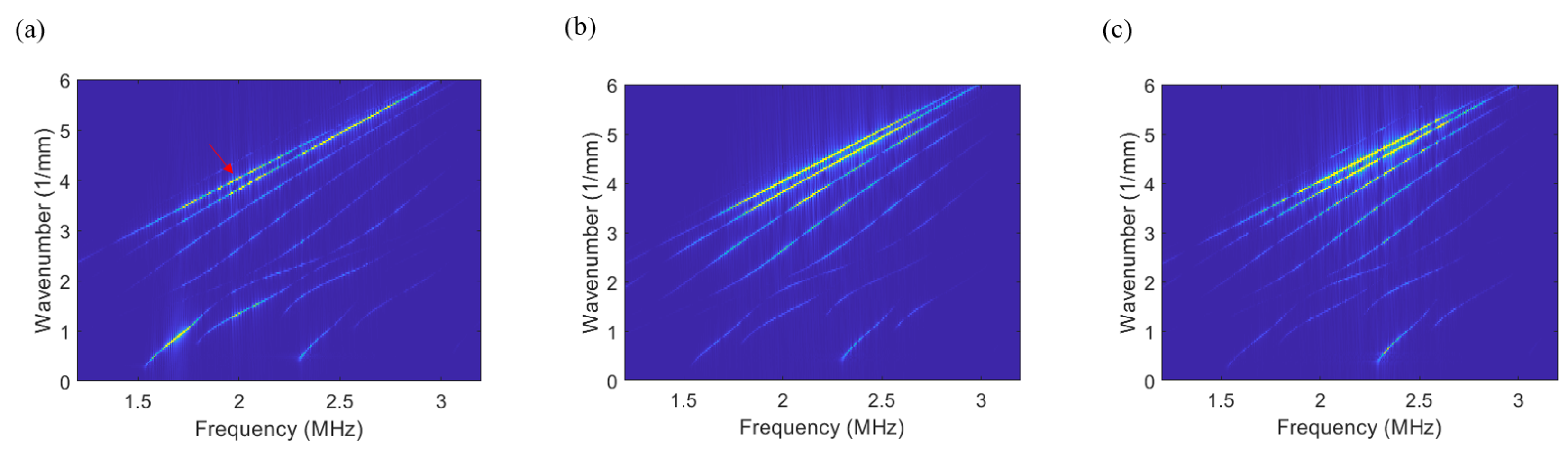
Figure 8 investigates the influence of excitation length and the number of force points on wave generation. Increasing the number of force points from 21 to 101, as shown in
Figure 8a,b, extends the excitation length from 10 to 50 wavelengths, significantly enhancing the generation of the desired wave mode. The desired wave mode is indicated in
Figure 8a. However, further increasing the spacing between force points, as illustrated in
Figure 8c, extends the excitation length to 100 wavelengths with limited additional improvement. Based on these findings, the configuration in
Figure 8b is adopted for subsequent analyses. Building upon the optimized excitation configuration,
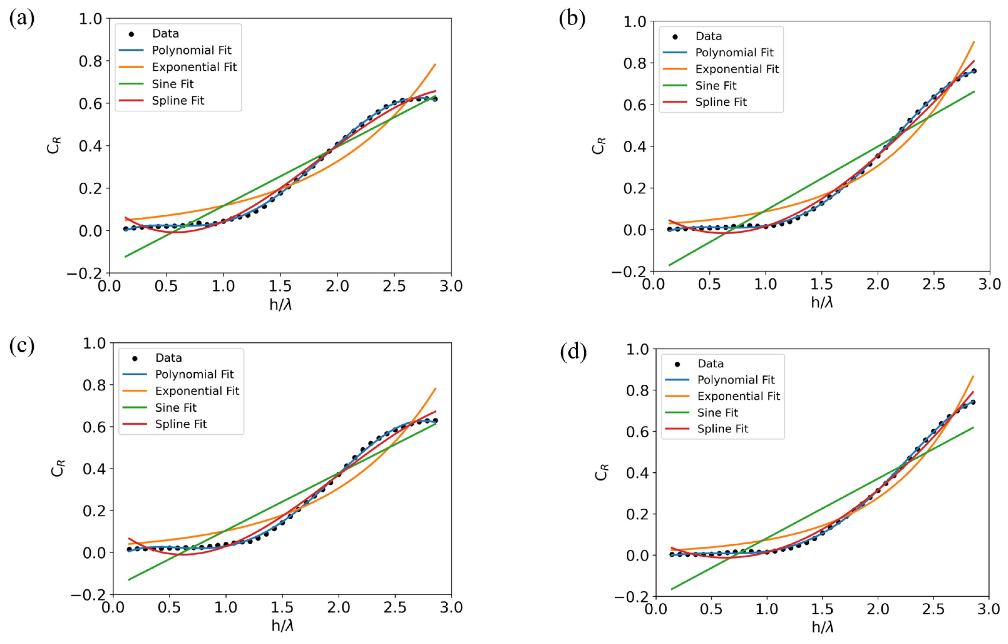
Figure 9 examines the reflection coefficients of HOMC as a function of the ratio of defect depth to wavelength. The analysis distinguishes between cases where the defect width is larger than one wavelength (
Figure 9a,b) and those where it is smaller (
Figure 9c,d). To model this relationship, four curve-fitting approaches—polynomial, exponential, sine, and spline—were evaluated. The polynomial fit outperforms the others, demonstrating superior accuracy and serving as the basis for comparison with machine learning models. Detailed parameters of these fitted curves are summarized in
Table 1.
Figure 10 explores the correlation between defect depth and reflection coefficients. The results show minor differences between cases with larger and smaller defect widths relative to the wavelength. This trend remains consistent across receiver placements on both the upper and lower surfaces. Based on this observation, machine learning models were developed. These models were trained on data from defects with larger widths (w = 1 mm) to predict the depth of defects with smaller widths (w = 0.5 mm).
3.3. Machine Learning Enhanced Inspection of Sharp Notches
PCA was employed for feature extraction and selection within the proposed ML method framework. Its primary function is to reduce the dimensionality of the feature space while retaining the most significant features for accurate depth prediction based on reflected waves.
Figure 11 illustrates the cumulative explained variance ratio as a function of the number of principal components (PCs) for the training dataset. The curve shows a rapid increase in explained variance with the first eight PCs, followed by a plateau as additional PCs are included. For both the top and bottom surfaces, a cumulative explained variance of 95% is achieved with just five PCs, indicating that these components capture the majority of the variance. Beyond this threshold, the contribution of additional PCs to the variance is minimal, suggesting that dimensionality can be effectively reduced to five PCs without significant loss of information. Consequently, five PCs were selected as input features for the ML models.
The performance of five commonly used ML models for sharp defect depth prediction was compared, alongside the linear regression (LR) method. To optimize the prediction capabilities of each model, key hyperparameters were selected and fine-tuned using random search. The selection of hyperparameters was informed by trial tests and existing recommendations in the literature [
24,
25]. The prediction performance of all regression models, both pre- and post-tuning, is presented to demonstrate the impact of hyperparameter tuning. A fivefold cross-validation approach was used to evaluate the models. The final performance metric is the average of the performance measures from the validation sets across all iterations.
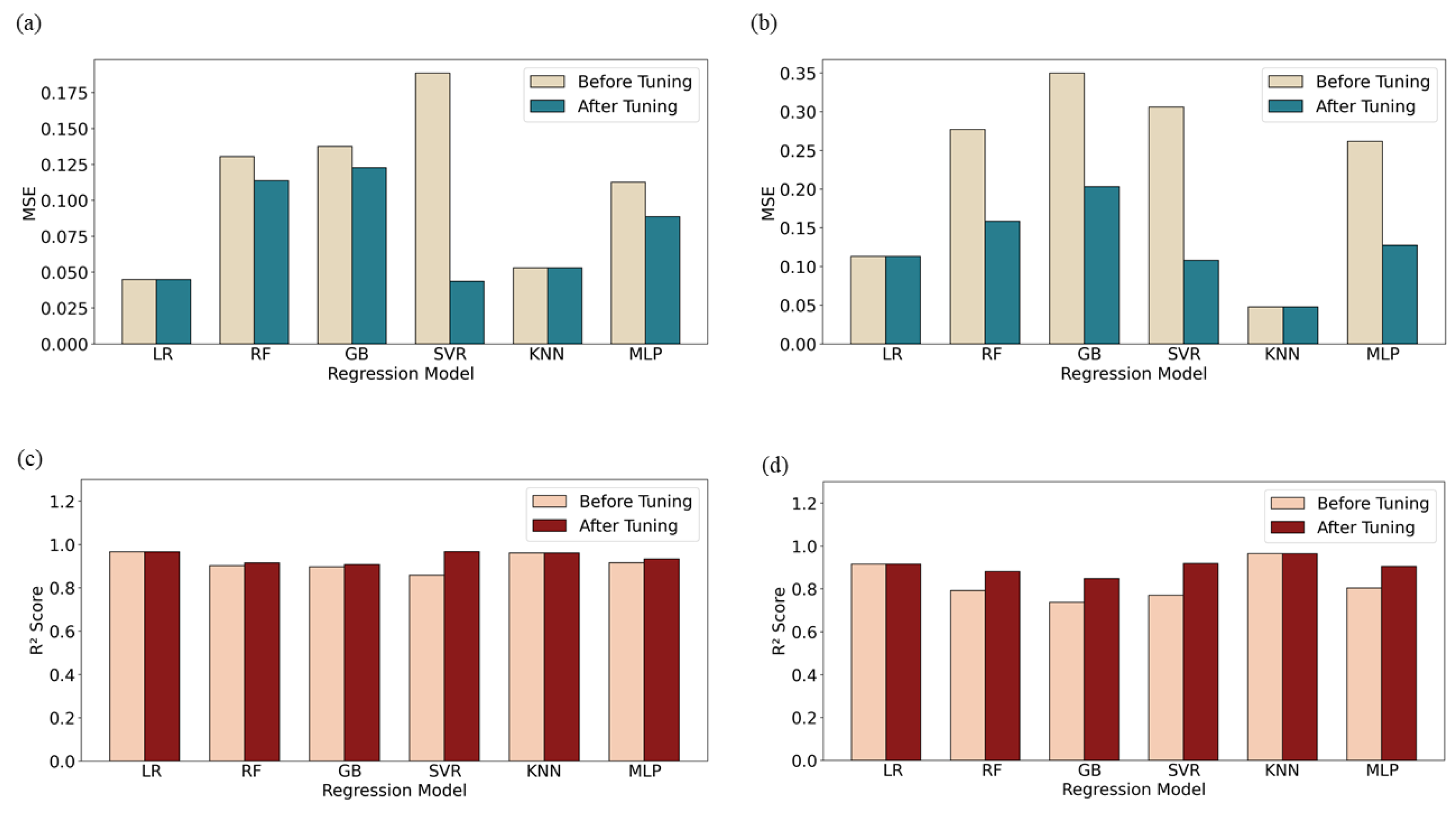
Figure 12 compares the average mean squared error (MSE) and coefficient of determination (
) score of all regression algorithms before and after tuning for depth prediction on the validation set. Without tuning, both LR and KNN significantly outperform the other regression models. After tuning, the performance of SVR improves substantially, becoming comparable to that of LR and KNN. Among all models, the SVR algorithm shows the highest sensitivity to hyperparameter tuning, with the MSE decreasing by 76.9% for the top surface (
Figure 12a) and 64.7% for the bottom surface (
Figure 12b). In addition, the
score increases by 12.7% for the top surface (
Figure 12c) and 19.3% for the bottom surface (
Figure 12d). In contrast, KNN shows the least sensitivity to hyperparameter tuning. Nevertheless, it consistently ranks among the top three most accurate models, regardless of tuning or whether the data are from the top or bottom surface. Moreover, KNN outperforms LR on the bottom surface, reinforcing its position as a strong candidate for comparison with the polynomial fitting results.
To demonstrate the versatility of the proposed method, the fitting model and machine learning model were trained using data from defects with a width of 1 mm (greater than one wavelength) and subsequently used to predict the depths of defects with a width of 0.5 mm (less than one wavelength).
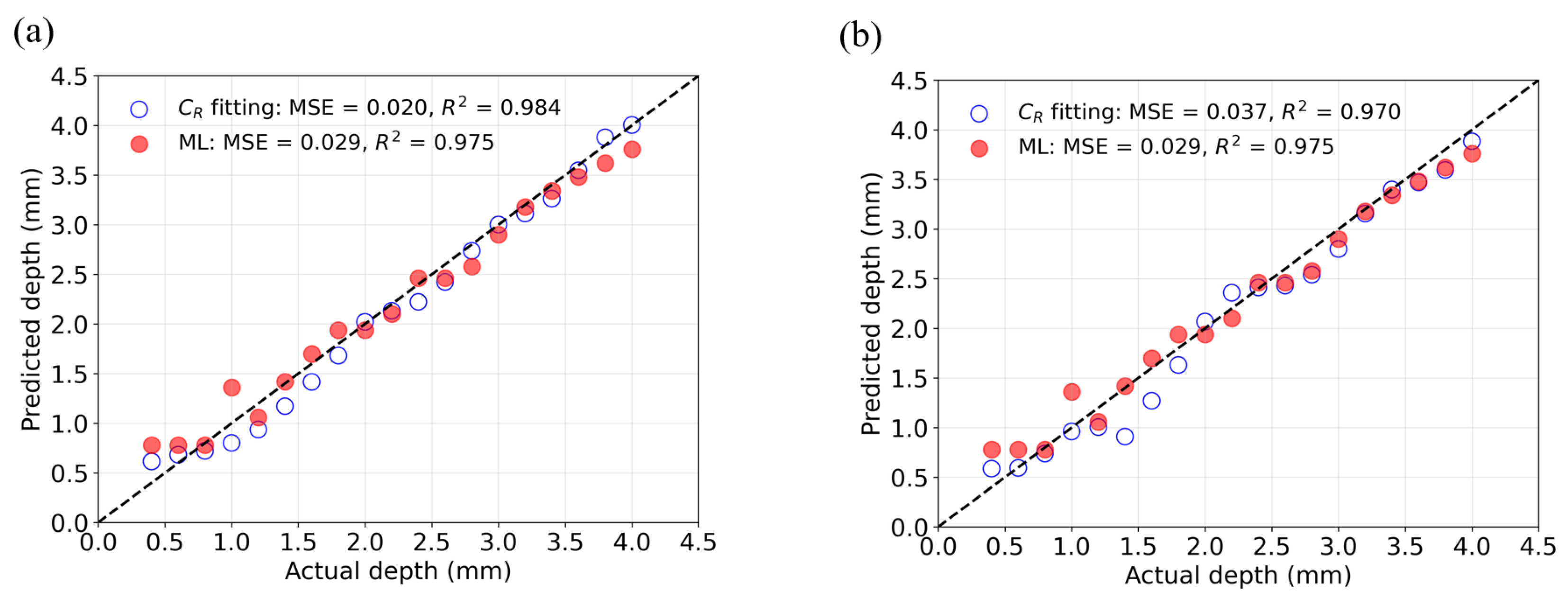
Figure 13 presents a comparison of the performance of the fitting model and the ML model in predicting defect depths. The dashed line represents the ideal prediction, where the predicted values perfectly align with the actual values. Predictions from the fitting model using
are shown as blue hollow circles, while predictions from the ML model are depicted as red solid circles. When signals are acquired from the top surface, the fitting method demonstrates slightly higher prediction accuracy, reflected by a lower MSE and a higher
value compared to the ML model. Conversely, when signals are obtained from the bottom surface, the ML model exhibits superior predictive performance. However, for both methods, the prediction accuracy improves as the defect depth increases.
4. Discussion
This study highlights the advantages of using HOMC guided waves for inspecting structures with surface features and sharp, deep defects. HOMC waves lose much less energy than fundamental mode guided waves and Rayleigh waves when interacting with complex surface conditions, attributed to reduced surface motion. Their shorter wavelengths also provide enhanced resolution for detecting sharp defects. This study demonstrates that HOMC waves can effectively characterize notches up to three wavelengths deep, corresponding to 50% of the structure’s thickness, in T-joint configurations.
Both conventional fitting models and machine learning models, utilizing reflected wave signals, demonstrated the ability to measure the depth of sharp defects, especially those deeper than 18% of the structural thickness. Reflected waves were selected due to limited structural access, which often prevents transducer placement on both sides. Both methods could predict defect depths across varying defect widths. This study showed that a model trained on wider defects could also estimate the depth of narrower defects, even when their width was reduced by half. This capability is especially valuable for pitting corrosion, where defects tend to be narrow and deep. Although both the conventional and ML methods attained comparable prediction accuracy, ML approaches offer certain potential advantages. While using a single scalar (reflection or transmission) is simple, it relies on a priori knowledge about how to gate signals and on specific assumptions about wave modes. By contrast, an ML model can automatically learn subtle features in the time domain or frequency domain, such as amplitude envelopes or phase shifts, reducing the burden of manual signal processing. Moreover, ML can flexibly handle a wide range of defect shapes or even multiple overlapping defects, a scenario in which conventional reflection/transmission methods become more complex. For instance, pitting corrosion with varying depth-to-width ratios would require detailed gating or curve fitting, whereas an ML approach may more readily adapt to such variability. Future research will focus on investigating the ability of the proposed inspection method to evaluate such defects, enabling a more realistic assessment of structural integrity.
However, in our 2D simulations, these potential gains of ML methods were not fully realized because the wave interactions were relatively clean and the feature sets were limited, conditions under which scalar coefficients still performed effectively. In real world scenarios, ML methods can be vulnerable to noise and require substantial amounts of high quality training data. They also involve added computational complexity, which may not be worthwhile if reflection and transmission peaks alone are sufficient for defect detection. Consequently, while ML may offer clear benefits for complicated defects or multiple parameter analyses, a straightforward reflection or transmission coefficient approach remains more practical for many industrial inspections. Future work will focus on refining the machine learning approach by expanding the training data, incorporating noise augmentation, and optimizing both the input features and the machine learning models.
5. Conclusions
This study evaluates the use of higher order modes cluster guided waves for detecting and quantifying sharp defects in structures, with a focus on surface features and deep defects. The results demonstrate that HOMC waves offer significant advantages over other guided wave modes, such as Rayleigh waves, A0, and S0 Lamb waves, due to their reduced surface motion. By leveraging reflected wave signals, both conventional fitting models and ML models accurately measured the depth of sharp deep defects. Importantly, this study demonstrates that models trained on wide defects can successfully predict the depths of narrower defects, highlighting the method’s applicability to pitting corrosion, where defects are typically narrow and deep. While both approaches achieved comparable prediction accuracy, ML models exhibit a clear advantage by reducing reliance on domain expertise, as they do not require manual configuration of signal gates. In conclusion, this paper demonstrates the effectiveness of the proposed method for the depth gauging of sharp, deep defects, establishing its potential for addressing complex challenges in structural health monitoring and non-destructive testing.
Author Contributions
Conceptualization, J.X.; methodology, J.X.; validation, J.X.; formal analysis, J.X.; investigation, J.X.; resources, J.X.; writing—original draft preparation, J.X.; writing—review and editing, J.X. and F.C.; visualization, J.X.; supervision, F.C.; project administrationn, F.C. All authors have read and agreed to the published version of the manuscript.
Funding
This research received no external funding.
Data Availability Statement
The original contributions presented in this study are included in the article. Further inquiries can be directed to the corresponding author.
Conflicts of Interest
The authors declare no conflicts of interest.
References
- Lowe, M.J.; Cawley, P.; Kao, J.; Diligent, O. The low frequency reflection characteristics of the fundamental antisymmetric Lamb wave a 0 from a rectangular notch in a plate. J. Acoust. Soc. Am. 2002, 112, 2612–2622. [Google Scholar] [CrossRef] [PubMed]
- Demma, A.; Cawley, P.; Lowe, M. Scattering of the fundamental shear horizontal mode from steps and notches in plates. J. Acoust. Soc. Am. 2003, 113, 1880–1891. [Google Scholar] [CrossRef] [PubMed]
- Rose, J.L.; Avioli, M.J.; Mudge, P.; Sanderson, R. Guided wave inspection potential of defects in rail. NDT & E Int. 2004, 37, 153–161. [Google Scholar]
- Lematre, M.; Lethiecq, M. Enhancement of guided wave detection and measurement in buried layers of multilayered structures using a new design of V(z) acoustic transducers. Acoustics 2022, 4, 996–1012. [Google Scholar] [CrossRef]
- Masserey, B.; Raemy, C.; Fromme, P. High-frequency guided ultrasonic waves for hidden defect detection in multi-layered aircraft structures. Ultrasonics 2014, 54, 1720–1728. [Google Scholar] [CrossRef]
- Zhang, X.; Li, B.; Zhang, X.; Song, X.; Tu, J.; Cai, C.; Yuan, J.; Wu, Q. Internal and external pipe defect characterization via high-frequency Lamb waves generated by unidirectional EMAT. Sensors 2023, 23, 8843. [Google Scholar] [CrossRef]
- Jayaraman, C.; Krishnamurthy, C.; Balasubramaniam, K. Higher Order modes cluster (homc) guided waves—A new technique for ndt inspection. AIP Conf. Proc. 2009, 1096, 121–128. [Google Scholar]
- Ratnam, D.; Balasubramaniam, K.; Maxfield, B.W. Generation and detection of higher-order mode clusters of guided waves (HOMC-GW) using meander-coil EMATs. IEEE Trans. Ultrason. Ferroelectr. Freq. Control 2012, 59, 727–737. [Google Scholar] [CrossRef]
- Rajagopal, P.; Balasubramaniam, K.; Hill, S.; Dixon, S. Interaction of Higher Order Modes Cluster (HOMC) guided waves with notch-like defects in plates. AIP Conf. Proc. 2017, 1806, 030015. [Google Scholar]
- Abbasi, Z.; Honarvar, F. Evaluation of the sensitivity of higher order modes cluster (HOMC) guided waves to plate defects. Appl. Acoust. 2022, 187, 108512. [Google Scholar] [CrossRef]
- Reddy, S.H.K.; Vasudevan, A.; Rajagopal, P.; Balasubramaniam, K. Scattering of Higher Order Mode Clusters (HOMC) from surface breaking notches in plates with application to higher temperature gradients. NDT & E Int. 2021, 120, 102441. [Google Scholar]
- Satyarnarayan, L.; Chandrasekaran, J.; Maxfield, B.; Balasubramaniam, K. Circumferential higher order guided wave modes for the detection and sizing of cracks and pinholes in pipe support regions. NDT & E Int. 2008, 41, 32–43. [Google Scholar]
- Chandrasekaran, J.; Krishnamurthy, C.; Balasubramaniam, K. Axial Higher Order Modes Cluster (A-HOMC) Guided Wave for Pipe Inspection. AIP Conf. Proc. 2010, 1211, 161–168. [Google Scholar]
- Khalili, P.; Cawley, P. Excitation of single-mode Lamb waves at high-frequency-thickness products. IEEE Trans. Ultrason. Ferroelectr. Freq. Control 2015, 63, 303–312. [Google Scholar] [CrossRef] [PubMed]
- Zhang, K.; Lv, G.; Guo, S.; Chen, D.; Liu, Y.; Feng, W. Evaluation of subsurface defects in metallic structures using laser ultrasonic technique and genetic algorithm-back propagation neural network. NDT & E Int. 2020, 116, 102339. [Google Scholar]
- Dworakowski, Z.; Ambrozinski, L.; Packo, P.; Dragan, K.; Stepinski, T. Application of artificial neural networks for compounding multiple damage indices in Lamb-wave-based damage detection. Struct. Control Health Monit. 2015, 22, 50–61. [Google Scholar] [CrossRef]
- Huber, A. The Dispersion Calculator: A Free Software for Calculating Dispersion Curves of Guided Waves. In Proceedings of the 20th World Conference on Non-Destructive Testing (WCNDT 2024), NDT. net, Incheon, Republic of Korea, 27–31 May 2024; Volume 29, pp. 1–17. [Google Scholar]
- Liu, M.; Zhang, W.; Chen, X.; Li, L.; Wang, K.; Wang, H.; Cui, F.; Su, Z. Modelling guided waves in acoustoelastic and complex waveguides: From SAFE theory to an open-source tool. Ultrasonics 2024, 136, 107144. [Google Scholar] [CrossRef]
- Khalili, P.; Cegla, F. Excitation of single-mode shear-horizontal guided waves and evaluation of their sensitivity to very shallow crack-like defects. IEEE Trans. Ultrason. Ferroelectr. Freq. Control 2020, 68, 818–828. [Google Scholar] [CrossRef]
- Xiao, J.; Chen, J.; Yu, X.; Lisevych, D.; Fan, Z. Remote characterization of surface slots by enhanced laser-generated ultrasonic Rayleigh waves. Ultrasonics 2022, 119, 106595. [Google Scholar] [CrossRef]
- Rajagopal, P.; Drozdz, M.; Skelton, E.A.; Lowe, M.J.; Craster, R.V. On the use of absorbing layers to simulate the propagation of elastic waves in unbounded isotropic media using commercially available finite element packages. NDT & E Int. 2012, 51, 30–40. [Google Scholar]
- Yao, H.; Tian, L. A genetic-algorithm-based selective principal component analysis (GA-SPCA) method for high-dimensional data feature extraction. IEEE Trans. Geosci. Remote Sens. 2003, 41, 1469–1478. [Google Scholar]
- Bergstra, J.; Bengio, Y. Random search for hyper-parameter optimization. J. Mach. Learn. Res. 2012, 13, 281–305. [Google Scholar]
- Tian, J.; Qi, C.; Peng, K.; Sun, Y.; Mundher Yaseen, Z. Improved permeability prediction of porous media by feature selection and machine learning methods comparison. J. Comput. Civ. Eng. 2022, 36, 04021040. [Google Scholar] [CrossRef]
- Xiao, J.; Cui, F. Machine learning enhanced characterization of surface defects using ultrasonic Rayleigh waves. NDT & E Int. 2023, 140, 102969. [Google Scholar]
Figure 1.
(a) Phase velocity dispersion curves for the first eight Lamb wave modes in an 8 mm aluminum plate, and (b) deflected shapes of the A1 mode in the same aluminum plate.
Figure 1.
(a) Phase velocity dispersion curves for the first eight Lamb wave modes in an 8 mm aluminum plate, and (b) deflected shapes of the A1 mode in the same aluminum plate.
Figure 2.
Schematic of the 2D FE setup for a T-joint using an angled wedge.
Figure 2.
Schematic of the 2D FE setup for a T-joint using an angled wedge.
Figure 3.
Schematic of the 2D FE setup for ML studies on sharp defect inspection.
Figure 3.
Schematic of the 2D FE setup for ML studies on sharp defect inspection.
Figure 4.
The flow chart of the proposed ML method for sharp defect depth gauging.
Figure 4.
The flow chart of the proposed ML method for sharp defect depth gauging.
Figure 5.
FE displacement magnitude contours (blue: low; yellow: high) of HOMC guided waves on T-joints at t = (a) 150 μs, (b) 180 μs, and (c) 210 μs.
Figure 5.
FE displacement magnitude contours (blue: low; yellow: high) of HOMC guided waves on T-joints at t = (a) 150 μs, (b) 180 μs, and (c) 210 μs.
Figure 6.
Time-domain signals recorded at four locations: (a) intact T-joint, after weld; (b) T-joint with a -deep defect, after weld; (c) intact T-joint, before weld; and (d) T-joint with a -deep defect, before weld.
Figure 6.
Time-domain signals recorded at four locations: (a) intact T-joint, after weld; (b) T-joint with a -deep defect, after weld; (c) intact T-joint, before weld; and (d) T-joint with a -deep defect, before weld.
Figure 7.
Two-dimensional FE predictions of (a) transmission and (b) reflection coefficients for T-joint defect inspection using HOMC guided waves.
Figure 7.
Two-dimensional FE predictions of (a) transmission and (b) reflection coefficients for T-joint defect inspection using HOMC guided waves.
Figure 8.
Two-dimensional FFT color plots (blue: low; yellow: high) of the out-of-plane displacement signals received along the plate surface, illustrating three excitation configurations: (a) 21 point forces, (b) 101 point forces, and (c) 101 point forces with double spacing between forces.
Figure 8.
Two-dimensional FFT color plots (blue: low; yellow: high) of the out-of-plane displacement signals received along the plate surface, illustrating three excitation configurations: (a) 21 point forces, (b) 101 point forces, and (c) 101 point forces with double spacing between forces.
Figure 9.
Comparison of curve-fitting methods using reflection coefficients obtained by line scans on (a) the top surface of the plate with w , (b) the bottom surface of the plate with w , (c) the top surface of the plate with w , and (d) the bottom surface of the plate with w .
Figure 9.
Comparison of curve-fitting methods using reflection coefficients obtained by line scans on (a) the top surface of the plate with w , (b) the bottom surface of the plate with w , (c) the top surface of the plate with w , and (d) the bottom surface of the plate with w .
Figure 10.
Discrepancies in the correlation between defect depth and reflection coefficient for w and w : (a) received points on the top surface and (b) received points on the bottom surface.
Figure 10.
Discrepancies in the correlation between defect depth and reflection coefficient for w and w : (a) received points on the top surface and (b) received points on the bottom surface.
Figure 11.
Cumulative explained variance ratio of principal components derived from PCA applied to reflected wave features from (a) the top surface and (b) the bottom surface of the plate.
Figure 11.
Cumulative explained variance ratio of principal components derived from PCA applied to reflected wave features from (a) the top surface and (b) the bottom surface of the plate.
Figure 12.
(a) Mean squared error for the top surface, (b) mean squared error for the bottom surface, (c) coefficient of determination for the top surface, and (d) coefficient of determination for the bottom surface, for all regression models before and after tuning on the validation dataset.
Figure 12.
(a) Mean squared error for the top surface, (b) mean squared error for the bottom surface, (c) coefficient of determination for the top surface, and (d) coefficient of determination for the bottom surface, for all regression models before and after tuning on the validation dataset.
Figure 13.
Comparison of the fitting model and ML model for defect depth prediction: (a) received signals from the top surface and (b) received signals from the bottom surface.
Figure 13.
Comparison of the fitting model and ML model for defect depth prediction: (a) received signals from the top surface and (b) received signals from the bottom surface.
Table 1.
Parameters of fitted curves.
Table 1.
Parameters of fitted curves.
| Location of Receivers | | | | | | |
|---|
| w & upper surface | | | | | | |
| w & lower surface | | | | | | |
| w & upper surface | | | | | | |
| w & lower surface | | | | | | |
| Disclaimer/Publisher’s Note: The statements, opinions and data contained in all publications are solely those of the individual author(s) and contributor(s) and not of MDPI and/or the editor(s). MDPI and/or the editor(s) disclaim responsibility for any injury to people or property resulting from any ideas, methods, instructions or products referred to in the content. |
© 2025 by the authors. Licensee MDPI, Basel, Switzerland. This article is an open access article distributed under the terms and conditions of the Creative Commons Attribution (CC BY) license (https://creativecommons.org/licenses/by/4.0/).


