Resonant Metasurfaces with a Tangential Impedance

Abstract

Metasurfaces formed by monopole and dipole resonators are studied theoretically. The monopole resonators are Helmholtz resonators or membranes vibrating on the first eigenfrequency; the dipole ones are spheres on springs or membranes vibrating on the second eigenfrequency. It is shown that acoustic properties of the metasurface formed by the built-in monopole resonators can be described by an equivalent impedance, which characterizes a normal forcing to the surface, whereas this impedance is not suitable for the metasurface formed by the dipole resonators, because motion of the metasurface is excited by a forcing tangential to the surface. For such boundaries, a new characteristic named “tangential impedance” is proposed. This is a ratio of the second derivative of the sound pressure along a coordinate tangential to the boundary to the normal velocity of the boundary. The dipole metasurface can be described by the equivalent tangential impedance. Reflection and absorption coefficients of the surface with the tangential impedance are found for a harmonic plane wave in dependance of an incidence angle. It is found that the angular dependences of the coefficients are very different for the monopole and dipole metasurfaces.

1. Introduction

A number of papers devoted to acoustic metamaterials is growing rapidly every year. Lists of references in reviews [1,2,3,4] observing recent achievements show the development of the metamaterials, their properties and areas of possible applications. Usually, the metamaterials are artificial structures consisting of similar elements with small wave dimensions, which can have specific properties. In most cases, the elements are resonators of different types interacting with each other. A surface covering the resonant elements can specifically react to an outer sound field; therefore, the surface is named a metasurface.

Resonant metasurfaces are being studied both theoretically and experimentally. One of the first applications was a sound-absorbing structure made of Helmholtz resonators [5], which is widely used for acoustic treatment in rooms today. At the macro-scale, an equivalent surface impedance was proposed [6] to simplify boundary conditions on the metasurfaces. Due to homogenization methods, a periodic array of the Helmholtz resonators can be described by the effective admittance depending on resonators’ parameters [7]. In the simplest structures, the resonators interact acoustically through the medium. Specific relations between neighbor resonators can change the effective impedance and, for example, increase the sound absorption efficiency [8].

Stretched membranes are successfully used for producing the metamaterials. Due to this technology, the metamaterial with the negative dynamic mass was experimentally realized [9]. Rigid masses attached to the membranes are used to change the natural frequencies and modes of the membrane elements [10,11]. Using the membranes with curved shapes allows for one to adjust their eigenfrequencies as well [12]. The metasurface manufactured from square membranes is proposed and studied in [13].

Specific acoustic properties of the metamaterials and metasurfaces appear in the vicinity of the resonant frequency of the elements. To enlarge the band, the resonators with different but close eigenfrequencies are applied. The inner volume and neck sizes of the Helmholtz resonator are varied in [14]. In case of quarter and half-wave resonators, their lengths are different [15]. Another way is to use actively controlled elements. The known techniques [16,17] propose to design electro-mechanical devices with resonant impedance on a wide-frequency band.

Often, the Helmhltz resonator is chosen as a meta-atom. It is a monopole secondary sound source; in other words, it is a source of the volume velocity. Another type of resonator was proposed in [18], which oscillates with constant volume. Thus, their volume velocity is zero, and they are sources of the force acting on the surrounding medium. The proposed oscillators were named “dipole resonators” because the radiated sound field has dipole characteristics. Then, the dipole resonators were successfully applied for reduction of noise radiated from an open duct [19]. A combination of the monopole and dipole resonators named “monopole–dipole resonator” is an effective absorber for narrow pipes [20,21] and waveguides [22] and in planar arrays [23]. The surfaces covered by the dipole resonators have not yet been studied, with the exception of a recent paper [24] investigating sound propagation in a narrow waveguide lined with identical dipole resonators.

This paper focuses on the theoretical understanding of acoustic properties of the metasurfaces formed by means of the dipole resonators. We consider two types of resonators: the first one is the mechanical oscillator, and the second one is the membrane-type cell. On the basis of the obtained results, we propose a new characteristic for the metasurfaces with specific features. The problem is formulated to obtain an exact and physically clear solution analytically, but the study of more complex systems requires applying numerical approaches, which are widely used for research in acoustic metamaterials [25,26,27].

2. Resonator-Based Metasurfaces

To understand the fundamental aspects, it is enough to consider the problem of sound propagation in two-dimensional space and its interaction with a one-dimensional boundary. We start with the surface with the Helmholtz resonators (for brevity, called simply the monopole metasurface hereafter), and then, we compare it with the surface covered by the dipole resonators called the dipole metasurface.

2.1. Monopole Resonators

2.1.1. Scattered Sound Field

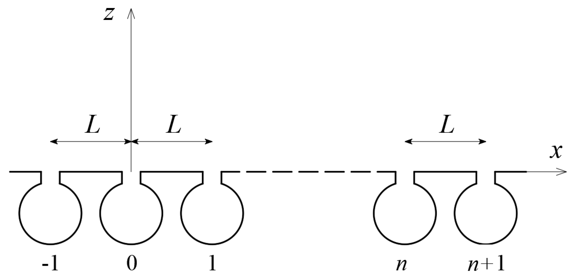
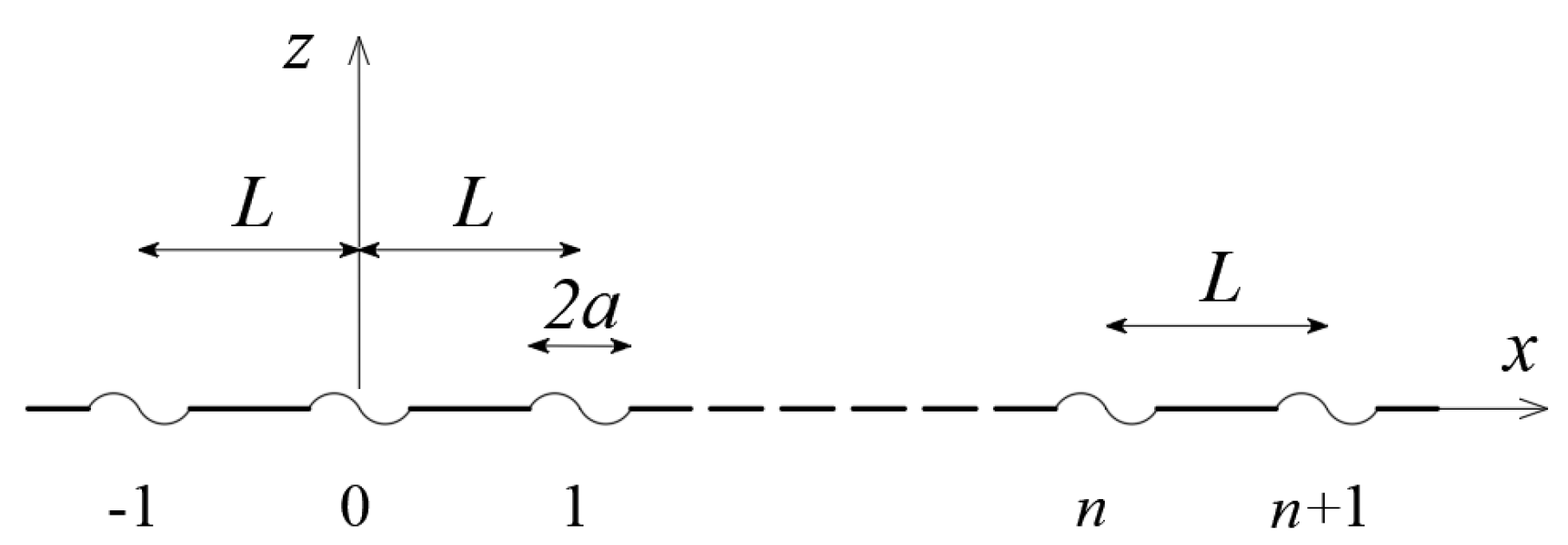
We now find the sound field scattered by a flat rigid surface with built-in Helmholtz resonators, which are monopoles. They are located periodically with a distance L as shown in Figure 1. We consider the two-dimensional problem; thus, the surface coincides with the plane $z=0$ and the resonators are at points $x_n=nL$, where $n$ is the number of the resonator. Assuming a time-harmonic disturbance in the form of $e^{-i\omega t}$, where t is time, and $\omega$ is an angular frequency, the sound pressure in the half space $z\ge 0$ can be given as follows

$$P\left(x,z\right)=A{e}^{i{\xi }_{0}x-i{\kappa }_{0}z}+A{e}^{i{\xi }_{0}x+i{\kappa }_{0}z}+P_1,$$

(1)

where ${\xi }_0$ and ${\kappa }_0$ are the components of the wave vector. The first term in the right part of (1) is the incident plane wave with an amplitude $A$, the second one is the reflected plane wave by the rigid surface, and $P_1$ is the sound field radiated by the resonators. In addition, we can introduce an incidence angle $\theta$; thus, ${\xi }_0=k\sin \theta$ and ${\kappa }_0=k\cos \theta$, where $k=\omega /c$, and $c$ is speed of sound.

First, we find the field $P_1$. Let the resonator with the number n be the volume velocity $Q_n$. According to the Bloch theorem, we can write $Q_n=Q{e}^{i{\xi }_{0}Ln}$ and then obtain the wave equation for point resonators.

$$\Delta P_1+k^2{P}_1=i\omega \rho Q{\displaystyle \sum }_n{e}^{i{\xi }_{0}Ln}\delta \left(x-nL\right)\delta \left(z\right)$$

(2)

where $\rho$ is the density of the medium.

The solution of (2) can be found by the Fourier method, giving the following result

$$P_1=\frac{\omega \rho Q}{L}\left(\frac{1}{{\kappa }_0}{e}^{i{\xi }_{0}x+i{\kappa }_{0}z}-i{\displaystyle \sum }_{m\ne 0}\frac{1}{{\eta }_m}{e}^{i{\xi }_{m}x-{\eta }_{m}z}\right),$$

(3)

where ${\xi }_m={\xi }_0+2\pi m/L$, ${\eta }_m=\sqrt{{\xi }_m^2-k^2}$.

The sound field (3) is a set of plane waves. If the distance between the resonators is less than a half-wavelength $L<\lambda /2$, where $\lambda =2\pi /k$, all waves with $m\ne 0$ are nonuniform and decay along the $z$-axis. Thus, the resonators radiate only the plane wave with $m=0$. Further, we consider only compact arrays with the period $L<\lambda /2$.

The equation of motion for the resonator with $n=0$ is

$$M\dot{Q}+\gamma Q+K\int Qdt=-\sigma P\left(0,0\right),$$

(4)

where $M$ and $K$ are the mass and stiffness of the Helmholtz resonator, $\gamma$ is the loss coefficient, and $\sigma$ is the cross-section area of its neck.

Substituting (1) into (4), we find the volume velocity of the resonator

$$Q=-\frac{2A}{Z+Z_r},$$

(5)

where $Z$ is the mechanical impedance of the Helmholtz resonator, and $Z_r$ is the radiation impedance of the monopole. These impedances are given by

$$Z=\frac{1}{\sigma }\left(\gamma -i\omega M+\frac{K}{-i\omega }\right),$$

(6)

$$Z_r=\frac{P_1\left(0,0\right)}{Q}=R+iX, R=\frac{\rho c}{L\cos \theta }, X=-\frac{\rho c}{L}{\displaystyle \sum }_{m\ne 0}\frac{k}{{\eta }_m}.$$

(7)

Expressions 1, 3 and 5 define the sound field scattered by the monopole metasurface.

2.1.2. Reflection Coefficient

The scattered field at a far distance is defined by two plane waves with the same wave vector. The first one is the wave reflected by the rigid surface; it is given by the second term in the right part of (1). The second one is the wave radiated by the array of the resonators; it is given by the first term in the brackets in (3). The running wave reflected by the metasurface is a superposition of these waves. Now, we can introduce the reflection coefficient as a ratio of the reflected wave amplitude to the incident one. From (1), (3), (5), (7), we obtain

$$V=\frac{Z+iX-R}{Z+iX+R}=\frac{\left(Z+iX\right)L\cos \theta -\rho c}{\left(Z+iX\right)L\cos \theta +\rho c}.$$

(8)

The resonance frequency ${\omega }_0$ of the Helmholtz resonator in the array can be found from the equation $\mathrm{Im}Z+X=0$. At frequencies significantly different from ${\omega }_0$, the impedance $\left|Z\right|\gg R,X$; hence, the reflection coefficient $V\approx 1$. This means that the resonators do not have an effect on the reflected field. Only near the resonance frequency is their effect significant. For example, the metasurface absorbs the incident wave at resonance frequency if the losses are optimal $\mathrm{Re}Z=R$.

2.1.3. Equivalent Impedance

A locally reacting surface can be characterized by the impedance, which is a ratio of the sound pressure to the normal velocity. A flat surface at the plane $z=0$ has the impedance $Z_{\perp }=P/v_z$, where $P$ is the sound pressure, $v_z$ is the normal velocity. The pressure forms a force acting normally on the surface. The force causes the surface to move; therefore, the surface reacts to normal impact and the sign “$\perp$” underlines this fact. It is natural to call the value $Z_{\perp }$ the normal impedance.

The reflection coefficient of the surface with the impedance $Z_{\perp }$ is

$$V=\frac{Z_{\perp }\cos \theta -\rho c}{Z_{\perp }\cos \theta +\rho c}.$$

(9)

Comparing (8) and (9), we can note that the metasurface reflects the incident plane wave like the uniform surface with the normal impedance $Z_{\perp }^{\prime }=\left(Z+iX\right)L$. Therefore, in order to characterize acoustic properties of the monopole metasurface, we can use the equivalent impedance $Z_{\perp }^{\prime }$. This means that at the far field, the metasurface behaves like an ordinary surface with the impedance $Z_{\perp }^{\prime }$, but the sound fields near the surfaces are very different.

The concept of the equivalent impedance can be useful to describe properties of complex planar systems. If the metasurface responds to the normal forcing, its equivalent impedance should be normal. In a general case, the equivalent impedance can be nonuniform.

2.2. Dipole Resonators

2.2.1. Scattered Sound Field

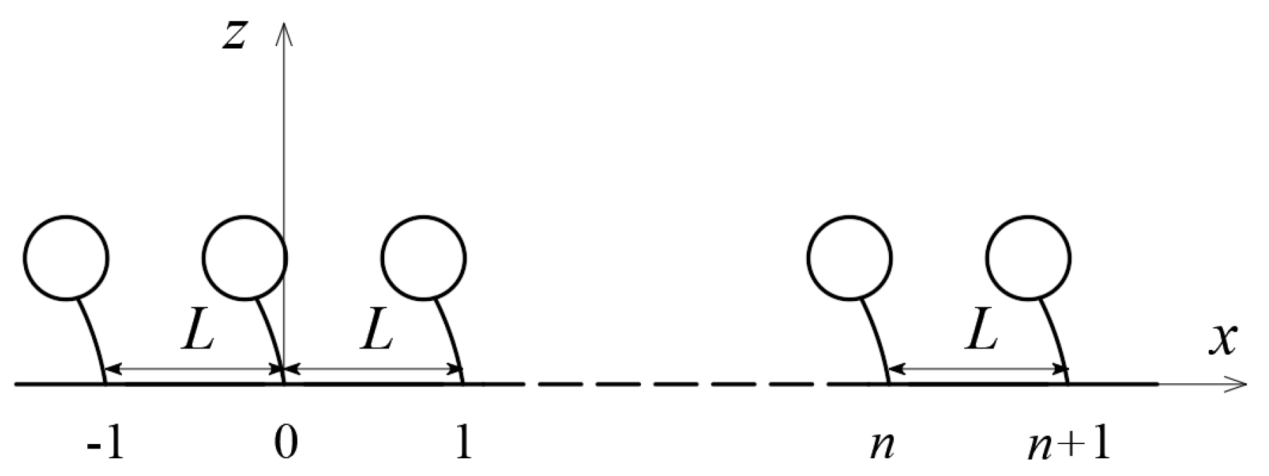
Now let us consider the similar metasurface, but we replace monopole resonators with dipole ones. The simplest model of the dipole resonator is an incompressible sphere on a spring [18]. The dipole metasurface is shown in Figure 2. The spheres can oscillate only along the $x$ axis; their radius and the height of the springs are small in comparison with the period $L$. Thus, the resonators can be considered as point dipole sound sources.

The resonator with the number $n$ has the dipole momentum $D_n=D{e}^{i{\xi }_{0}Ln}$. To find the sound field radiated by the dipoles $P_2$, the sound field of the monopoles (3) should be differentiated by the coordinate $x$. Thus, we can write

$$P_2=-\frac{i\omega \rho D}{L}\left(\frac{{\xi }_0}{{\kappa }_0}{e}^{i{\xi }_{0}x+i{\kappa }_{0}z}-i{\displaystyle \sum }_{m\ne 0}\frac{{\xi }_m}{{\eta }_m}{e}^{i{\xi }_{m}x-{\eta }_{m}z}\right).$$

(10)

The total sound field in the half space $z\ge 0$ is given by (1), where $P_1$ should be replaced by $P_2$.

In accordance with [24], the equation of motion for the resonator with $n=0$ has the form

$$M\dot{v}+\gamma v+K\int vdt=-\mu \left(\dot{v}-{\dot{u}}_x\right)+\rho \mathsf{\Omega }{\dot{u}}_x,$$

(11)

where $M$ and $\mathsf{\Omega }$ are the mass and the volume of the dipole, $K$ is the stiffness of the spring, $\gamma$ is the loss coefficient, $\mu$ is the attached mass, $v$ is the velocity of the dipole, $u_x$ is the velocity of the medium in the x-direction outside the dipole.

The velocity of the medium can be found from (1) and (10)

$$u_x=\frac{1}{i\omega \rho }{\left(\frac{\partial P}{\partial x}\right)}_{x=z=0}=2A\frac{{\xi }_0}{\omega \rho }-\frac{D}{L}\left(i\frac{{\xi }_0^2}{{\kappa }_0}+{\displaystyle \sum }_{m\ne 0}\frac{{\xi }_m^2}{{\eta }_m}\right).$$

(12)

The radiation impedance of the dipole is defined as a ratio of the force acting on the dipole along the x-axis $F_x=-\left(\mu +\rho \mathsf{\Omega }\right){\dot{u}}_x$ to its momentum, where $u_x$ is defined by (12). Thus, the radiation impedance of the dipole in the periodic array is

$$Z_r=\frac{F_x}{D}=R+iX, R=\frac{\omega {\xi }_0^2}{{\kappa }_{0}L}\left(\mu +\rho \mathsf{\Omega }\right), X=-\frac{\omega }{L}\left(\mu +\rho \mathsf{\Omega }\right){\displaystyle \sum }_{m\ne 0}\frac{{\xi }_m^2}{{\eta }_m}.$$

(13)

Note that Equations (11) and (13) are valid for dipoles of arbitrary form. The sphere with a radius $a$ and volume $\mathsf{\Omega }=\pi a^2$ moving along a rigid surface with the velocity $v$ has the attached mass $\mu =2\pi a^2\rho$ and the dipole momentum $D=4\pi a^{2}v$ [28].

Substituting (12) into (11), we find the dipole momentum of the resonator

$$D=-i{\xi }_0\frac{\mu +\rho \mathsf{\Omega }}{\rho }\frac{2A}{Z+Z_r},$$

(14)

$$Z=\frac{1}{4\pi a^2}\left(\gamma -i\omega \left(M+\mu \right)+\frac{K}{-i\omega }\right).$$

(15)

The sound field scattered by the dipole metasurface is defined by (10) and (14).

2.2.2. Reflection Coefficient

The real part of the radiation impedance (13) for the spherical dipole can be written in the following view

$$R=3\pi {\left(ka\right)}^2{\sin }^2\theta \frac{\rho c}{L\cos \theta }.$$

(16)

The far sound field consists of two plane waves; their superposition is the reflected field. From (1), (10), (14), we can find the reflection coefficient

$$V=\frac{Z+iX-R}{Z+iX+R}=\frac{\left(Z+iX\right)\frac{L}{3\pi {\left(ka\right)}^2}\cos \theta -\rho c{\sin }^2\theta }{\left(Z+iX\right)\frac{L}{3\pi {\left(ka\right)}^2}\cos \theta +\rho c{\sin }^2\theta }.$$

(17)

The angular dependances of the reflection coefficients for the monopole (8) and for the dipole (17) metasurfaces are significantly different. At normal incidence $\theta =0$, the reflection coefficient for the dipole surface is always equal to 1. The dipoles do not move if the wavevector of the incident wave is perpendicular to their momentums. In other words, the dipole metasurface does not respond to the normal impact and becomes absolutely rigid. The reflection coefficient is $V\approx 1$ at frequencies $\omega \ll {\omega }_0$ and $\omega \gg {\omega }_0$ as well. The metasurface absorbs the oblique incident wave under usual conditions $\mathrm{Im}Z=-X$ and $\mathrm{Re}Z=R$.

It is interesting that the monopole and dipole metasurfaces have the same reflection coefficients for the gliding incidence. If $\theta \to \pi /2$ from (8) and (17), we can find $V\to -1$. Thus, both metasurfaces behave like a soft boundary.

2.2.3. Equivalent Impedance

It is obvious that the usual impedance $Z_{\perp }$ is not suitable for describing the properties of the dipole metasurface, because its motion is produced by the tangential forcing. The metasurface moves if $\partial P/\partial x\ne 0$; therefore, the tangential impedance instead of the normal one should be used for such surfaces. To characterize the far sound field, we can formally introduce the parameter $Z_{\left|\right|}=\left(Z+iX\right)L/\left(3\pi {\left(ka\right)}^2\right)$, where the sign “$\left|\right|$” marks the tangential excitation, and find from (17) the reflection coefficient

$$V=\frac{Z_{\left|\right|}\cos \theta -\rho c{\sin }^2\theta }{Z_{\left|\right|}\cos \theta +\rho c{\sin }^2\theta }.$$

(18)

The tangential impedance is determined in Section 4. Now, we can see that the value $Z_{\left|\right|}$ is suitable as the equivalent impedance of the dipole metasurface.

3. Membrane-type Metasurfaces

3.1. Membrane in the Baffle

If the membrane lies in the plane $z=0$, its deflection $w$ in z-direction is given Equation [29]

$$T\frac{{\partial }^{2}w}{\partial x^2}-\varrho h\ddot{w}=-P,$$

(19)

where $h$, $\varrho$ and $T$ are the thickness, density and tension of the membrane, and $P$ is the sound pressure acting on the membrane. In (19), we suppose that the membrane is installed into a rigid infinite baffle. The sound wave acts on it from the half space $z>0$; on the other side of the membrane, the sound pressure is zero.

The membrane clamped at the points $x=\pm a$ has the first eigenfrequency ${\omega }_1$ and eigenmode $w_1$, which are

$${\omega }_1=\frac{\pi }{2a}\sqrt{\frac{T}{\varrho h}}, w_1=\cos \frac{\pi x}{2a}.$$

(20)

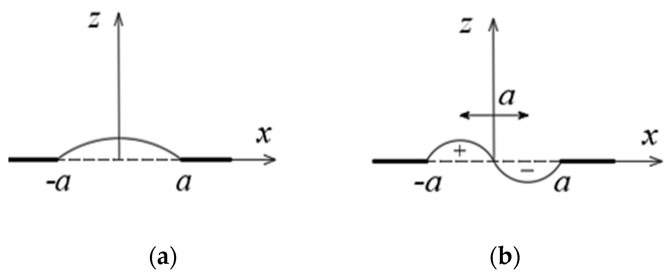
The second eigenfrequency and eigenmode are as follows

$${\omega }_2=\frac{\pi }{a}\sqrt{\frac{T}{\varrho h}}, w_2=\sin \frac{\pi x}{a}.$$

(21)

Figure 3 shows the first and the second eigenmodes of the membrane in the infinite baffle. It is obvious that the membrane is the source of the volume velocity at the first mode and behaves like a monopole if $ka\ll 1$. The second mode can be considered as two antiphase monopoles at distance $a$ from each other; the membrane radiates sound like a dipole.

Formally, we can use the results obtained in Section 2 for the monopole and dipole resonators for the membranes. However, we consider the problem of the membrane type metasurface separately. The first goal is to take into account the form of the oscillating surface, the second one is to find the solution for the membrane of an arbitrary size.

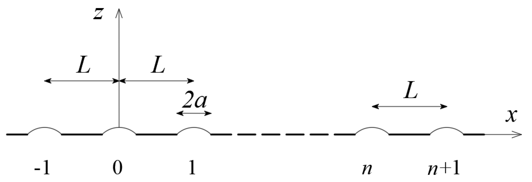
3.2. First Eigenmode

The membrane-type metasurface consists of the rigid surface with the installed periodic array of the membranes with the size $2a$, as shown in Figure 4. The centers of the membranes are at points $x_n=nL$. The total sound field at $z\ge 0$ is given by (1). We need to find the field $P_1$ scattered by the membranes.

Let the frequency $\omega$ of the incident wave be close to the first eigenfrequency ${\omega }_1$, defined by (20), and only the first eigenmode $w_1$ is excited by the sound field. Note that the exact solution for the membrane in the medium can be found, for example, in [30]. The velocity of the membrane with the number $n$ is $v_n=v{w}_1\left(x-nL\right)e^{i{\xi }_{0}Ln}$, $\left|x-nL\right|<a$. The sound field radiated by the membranes is found by the Fourier method

$$P_1=4\pi v\frac{\omega \rho a}{L}\left(\frac{f\left({\xi }_{0}a\right)}{{\kappa }_0}{e}^{i{\xi }_{0}x+i{\kappa }_{0}z}-i{\displaystyle \sum }_{m\ne 0}\frac{f\left({\xi }_{m}a\right)}{{\eta }_m}{e}^{i{\xi }_{m}x-{\eta }_{m}z}\right), f\left(x\right)=\frac{\cos x}{{\pi }^2-4x^2}.$$

(22)

From the equation of motion (19), where $w=v{w}_1$, and the pressure $P$ is taken from (1) with $P_1$ given by (22), we can find the velocity amplitude of the membrane with the number $n=0$

$$v=-4\pi \omega f\left({\xi }_{0}a\right)\frac{2A}{Z+Z_r},$$

(23)

where the mechanical impedance $Z$ and the radiation impedance $Z_r$ are defined by

$$Z=i\left(\varrho h{\omega }^2-T{\left(\frac{\pi }{2a}\right)}^2\right),$$

(24)

$$Z_r=R+iX, R=16{\pi }^2\frac{a{\omega }^2\rho }{L}\frac{f^2\left({\xi }_{0}a\right)}{{\kappa }_0}, X=-16{\pi }^2\frac{a{\omega }^2\rho }{L}{\displaystyle \sum }_{m\ne 0}\frac{f^2\left({\xi }_{m}a\right)}{{\eta }_m}.$$

(25)

Note that the losses in the membrane can be taken into account by using the complex value $T$, in which the image part is a loss factor [31].

If the membrane is small in comparison with the wavelength, i.e., $ka\ll 1$, then $f\left({\xi }_{0}a\right)\approx {\pi }^{-2}$, and the reflection coefficient is equal to

$$V=\frac{Z+iX-R}{Z+iX+R}=\frac{\left(Z+iX\right)\frac{{\pi }^{2}L}{16a\omega }\cos \theta -\rho c}{\left(Z+iX\right)\frac{{\pi }^{2}L}{16a\omega }\cos \theta +\rho c}.$$

(26)

We see that the reflection coefficients (8) and (26) have the same angular dependance. As expected, the surface with the membranes vibrating at the first eigenfrequency is the monopole metasurface with the equivalent normal impedance $Z_{\perp }^{\prime }=\left(Z+iX\right){\pi }^{2}L/\left(16a\omega \right)$.

3.3. Second Eigenmode

Now, we consider the array of the membranes vibrating at the second eigenfrequency (Figure 5). At $\omega \approx {\omega }_2$, we assume that the deflection of the membrane is strictly defined by the eigenmode $w_2$. Therefore, the velocities of the membranes are $v_n=v{w}_2\left(x-nL\right)e^{i{\xi }_{0}Ln}$, $\left|x-nL\right|<a$. Using the same calculations, we can find the following results.

The sound field radiated by the array is

$$\begin{gathered} P_2=-2\pi iv\frac{\omega \rho a}{L}\left(\frac{g\left({\xi }_{0}a\right)}{{\kappa }_0}{e}^{i{\xi }_{0}x+i{\kappa }_{0}z}-i{\displaystyle \sum }_{m\ne 0}\frac{g\left({\xi }_{m}a\right)}{{\eta }_m}{e}^{i{\xi }_{m}x-{\eta }_{m}z}\right), \\ g\left(x\right)=\frac{\sin x}{{\pi }^2-x^2}. \end{gathered}$$

(27)

By means of (27), the velocity amplitude can be found

$$v=-2\pi i\omega g\left({\xi }_{0}a\right)\frac{2A}{Z+Z_r}.$$

(28)

Now, the impedances are equal

$$Z=-i\left(\varrho h{\omega }^2-T{\left(\frac{\pi }{a}\right)}^2\right),$$

(29)

$$Z_r=R+iX, R=4{\pi }^2\frac{a{\omega }^2\rho }{L}\frac{g^2\left({\xi }_{0}a\right)}{{\kappa }_0}, X=-4{\pi }^2\frac{a{\omega }^2\rho }{L}{\displaystyle \sum }_{m\ne 0}\frac{g^2\left({\xi }_{m}a\right)}{{\eta }_m}.$$

(30)

With the approximation $g\left(x\right)\approx x/{\pi }^2$ if $x\ll 1$, the reflection coefficient is

$$V=\frac{Z+iX-R}{Z+iX+R}=\frac{\left(Z+iX\right)\frac{{\pi }^{2}L}{4c{\left(ka\right)}^3}\cos \theta -\rho c{\sin }^2\theta }{\left(Z+iX\right)\frac{{\pi }^{2}L}{4c{\left(ka\right)}^3}\cos \theta +\rho c{\sin }^2\theta }.$$

(31)

The dependance (31) coincides with (17) obtained for the dipole metasurface. Thus, the membrane-type metasurface can be characterized by the equivalent tangential impedance $Z_{\left|\right|}=\left(Z+iX\right){\pi }^{2}L/\left(4c{\left(ka\right)}^3\right)$.

Note that the membranes in both metasurfaces (Figure 4 and Figure 5) can be placed without gaps between each other. We should only suppose $L=2a$ to obtain the formulas for this case.

4. Tangential Impedance

4.1. Definition

Generally, the impedance is defined as the ratio of an external forcing on an object to a reaction of the object. In electricity, the external forcing is a voltage supplied to a circuit, and the reaction is a current in the circuit. In acoustics, the sound pressure acting on a boundary is considered as the forcing, whereas the velocity of the boundary is its reaction. Their ratio depends only on the acoustic properties of the boundary and is usually used as a boundary condition.

The ordinary definition of the impedance of a surface is $Z_{\perp }=P/v_n$, where $P$ is the sound pressure, and $v_n$ is the normal velocity of the surface. It is important that here we deal with the local impedance, which means that each point of the surface moves independently on the others. Above, we suggested to name the value $Z_{\perp }$ the normal impedance, because the pressure $P$ produces the force acting normally to the surface.

As shown in Section 2.2 and Section 3.3, there are specific surfaces, in which moving is caused by a forcing acting tangentially on the surface. The forcing acting on the dipole metasurface laying in the plane $z=0$ is proportional to the tangential component of the velocity $u_x~\partial P/\partial x$ of the medium near the surface. In addition, we have to remember that the field of the dipole array is found as the gradient in the x-direction. Thus, the forcing is proportional to the value ${\partial }^{2}P/\partial x^2$. The reaction of the surface can be described by the normal velocity $v_z$ in an ordinary way, because the tangential component of the surface velocity does not cause radiated waves in an inviscid medium.

Now, we can propose the value characterizing the impedance of the dipole metasurfaces as the ratio of ${\partial }^{2}P/\partial x^2$ to $v_z$. However, it would be convenient to have the dimension of the new impedance like the traditional one. The values ${\partial }^{2}P/\partial x^2$ and $P$ differ by a value proportional to the square of the distance. In the problem with the infinite plane, there is only one measure of the distance, which is the wavelength $\lambda$ or the wavenumber $k=2\pi /\lambda$. Finally, we can suggest the following definition of the tangential impedance for the dipole metasurface.

$$Z_{\left|\right|}=\frac{{\partial }^{2}P/\partial x^2}{-k^2{v}_z}.$$

(32)

Of course, the definition (32) is valid only for the harmonic plane wave. In general, the ratio $-\left({\partial }^{2}P/\partial x^2\right)/v_z$ is more appropriate for the tangential impedance, but it has a different dimension relative to $Z_{\perp }$.

4.2. Reflection Coefficient of a Plane Surface

The reflection coefficient of a plane wave incident on the plane surface can be found if the impedance of the surface is known. The surface characterized by the normal impedance $Z_{\perp }$ has the reflection coefficient given by (9). If the surface has the tangential impedance (32), the reflection coefficient can be calculated by means of (18).

Let us compare the angle dependances (9) and (18). At normal incidence, the reflection coefficient of the surface with the normal impedance is $V=\left(Z_{\perp }-\rho c\right)/\left(Z_{\perp }+\rho c\right)$, when $V=1$ for the surface with the tangential impedance. At gliding incidence, the surfaces of both types behave like a soft boundary because $V\to -1$. At oblique incidence, the sound wave is absorbed if $Z_{\perp }=\rho c/\cos \theta$ or $Z_{\left|\right|}=\rho c{\sin }^2\theta /\cos \theta$. For total absorption, both impedances should be real, and the normal impedance should be $Z_{\perp }\ge \rho c$. It is interesting that there is a value of the incidence angle $\theta$ for any value of $Z_{\left|\right|}$, when the wave is absorbed.

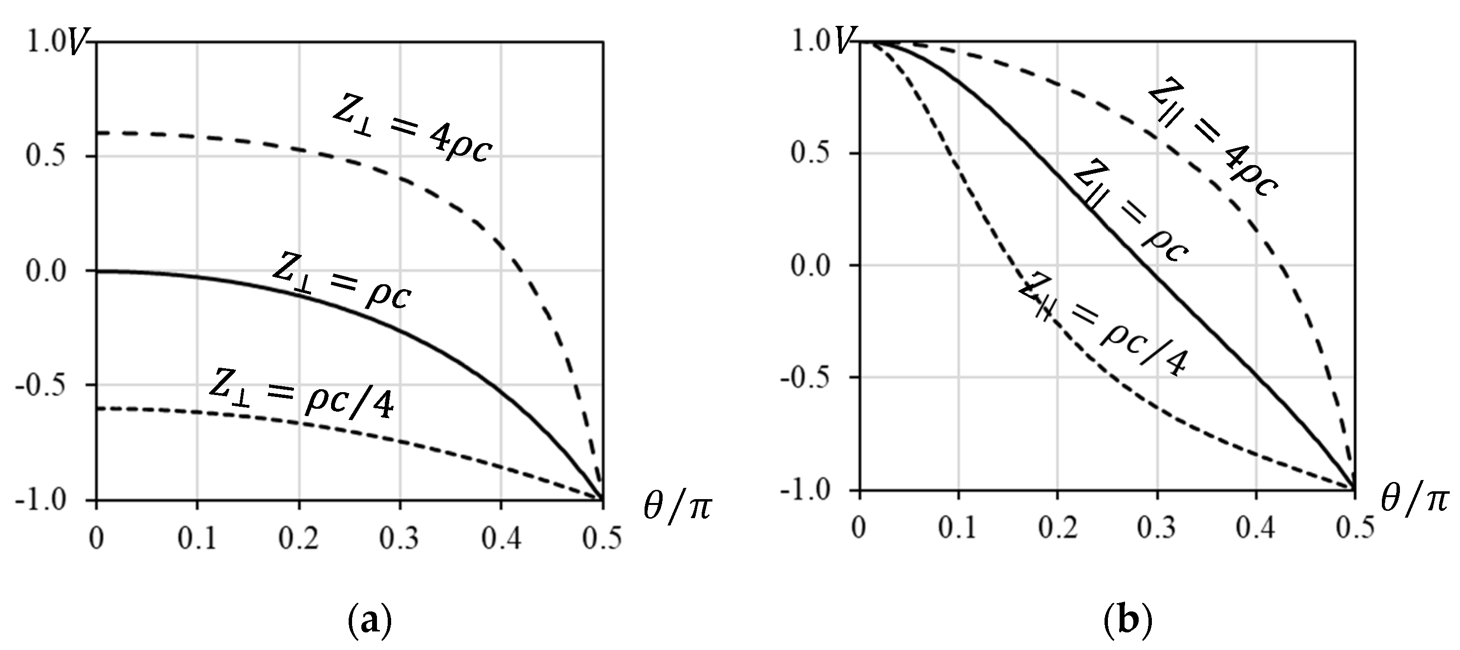
Figure 6 shows the dependances of the reflection coefficient on the incidence angle for some real values of the normal and tangential impedances. The impedances of the resonant metasurfaces are real if the resonant frequency found from the equations $\mathrm{Im}\left(Z_{\perp }+Z\right)=0$ or $\mathrm{Im}\left(Z_{\left|\right|}+Z\right)=0$ coincides with the frequency of the incident wave. The value of the real part can be adjusted by varying dissipation properties of the resonators. For example, the membranes could be manufactured from elastic materials with different loss coefficients, which are described by the image part of the modulus of elasticity.

The dependance for $Z_{\perp }$ is well known, the coefficient $V$ for $Z_{\left|\right|}$ varies from 1 to –1. By increasing the impedances $Z_{\perp }$ and $Z_{\left|\right|}$, the angle at which full absorption is provided tends to be $\pi /2$.

4.3. Diffuse Absorption Coefficient

In some cases, the metasurfaces could be used for sound absorption. The reflection coefficient $\alpha$ is connected with the absorption one by the relation $\alpha =1-{\left|V\right|}^2$. The surfaces with the impedances of both types can completely absorb the incident sound wave only at a certain angle. The absorption coefficient in the diffuse sound field is given by

$${\alpha }_d=\frac{2}{\pi }{{\displaystyle \int }}_0^{\frac{\pi }{2}}\alpha d\theta .$$

(33)

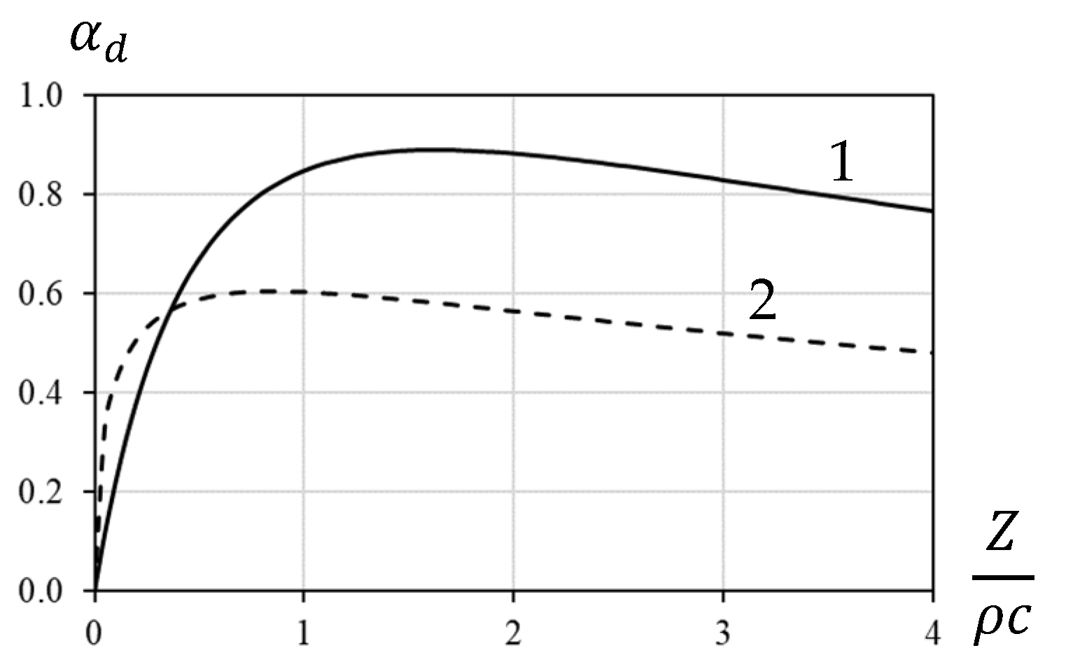
The diffuse absorption coefficient for the real values of the impedance is presented in Figure 7. Both curves have one maximum, which means that the absorption can be optimized. The surface with the normal impedance has the maximal absorption coefficient ${\alpha }_d=0.89$ if the impedance is $Z_{\perp }=1.63\rho c$. The same value for the tangential impedance surface is ${\alpha }_d=0.61$ at $Z_{\left|\right|}=0.86\rho c$. Thus, this type of the surface is a less efficient absorber; however, at low values, $Z<0.35\rho c$ has larger absorption coefficient.

5. Conclusions

We studied the acoustic properties of the surfaces with the integrated resonators located at a distance of less than a half-wavelength from each other. These surfaces are named “metasurfaces” because under some conditions, they have unusual acoustic characteristics.

Helmholtz resonators or membranes vibrating at the first eigenfrequency are monopole resonators; thus, their periodic array forms the monopole metasurface. To describe the sound reflection properties, one can use the ordinary impedance $Z_{\perp }$, which is the ratio of the pressure to the normal velocity of the surface. This means that the surface with the uniform impedance and the monopole metasurface produce the same reflected wave in the far field. In this sense, these surfaces are equivalent.

Another result takes place in the case of the dipole metasurface formed by spheres on springs or by membranes vibrating at the second eigenfrequency. The motion of the surface is excited by the velocity of the medium along the surface. In other words, the excitation does not occur normally, but tangentially. In particular, it causes the different dependences of the reflection coefficient on the incidence angle. Therefore, the impedance $Z_{\perp }$ is not suitable for the dipole metasurface.

For this reason, the concept of a tangential impedance is proposed. Calculations show that the exciting impact on the dipole metasurface is proportional to the second derivative of the pressure along the direction tangential to the surface. The definition of the tangential impedance $Z_{\left|\right|}$ for the dipole metasurface is given by (32). Using this parameter, we can obtain the reflection coefficient, which is found by means of the exact solution. Thus, the dipole metasurface is equivalent to the surface with the uniform impedance $Z_{\left|\right|}$.

The surfaces with the normal and tangential impedances have different reflective properties. The tangential impedance can be used to describe the acoustic properties of surfaces with a complex structure. It is important that definition (32) is valid only for the metasurfaces shown in Figure 2 and Figure 5. However, other metasurfaces may require a different definition of the tangential impedance.