1. Introduction
The vibration of a rail makes an essential contribution to railway rolling noise and has to be considered in any rolling noise model. One possible approach to modeling the dynamic behavior of a rail is a beam on an elastic foundation. This is appropriate as long as only frequencies below approximately 1.5 kHz [
1] and the excitation and propagation of bending waves are considered. The source of railway rolling noise is the interaction of wheels and rails at their point of contact, depending on the time and location. The contact between a rolling wheel and a rail can be accounted for as dynamic moving load.
While a moving load can be seen as an inherently time-dependent process, most available models for moving loads on beams are formulated in the frequency domain. The models proposed in [
2,
3,
4,
5] may serve as examples in which the response of infinite beams on a continuous or discrete elastic foundation was considered in the frequency domain. Frequency-domain models for wave propagation are essentially linear models. However, aside from purely linear excitation and propagation of structure-borne noise in a rail, nonlinear effects may be also important for both rolling noise generation [
6,
7,
8] and propagation [
9].
Nonlinear effects may still be considered in frequency-domain models in some special cases in which appropriate transformations are available. For example, the influence of nonlinearity in the viscoelastic foundations on the dynamic response of a beam can be analyzed [
9] by using such an approach. However, if a model takes into account multiple nonlinear effects, including those in the wheel–rail contact, it profits from an analysis in the time domain. A time-domain model for the dynamic response of a finite beam resting on a nonlinear viscoelastic foundation was reported in [
10], where a Runge–Kutta method based on a Galerkin approximation was used. However, for a rail, it is more appropriate if it is considered as an (effectively) infinite beam.
The elastic foundation of a beam represents the pads, sleepers, and ballasts or different constructions supporting the rail. Depending on the railway track type considered and the fidelity of the model, a number of different approaches to modeling the elastic foundation are available. Continuous single- and double-layer foundations [
8] were considered, as well as equidistant discrete supports (e.g., [
7,
11,
12,
13]). Some models also allow for variation of the properties, such as randomized spacing of the supports [
3,
14] or varying support stiffness [
14].
Higher-fidelity models for bending waves in beams on elastic foundations can be obtained with the finite element method (FEM). Frequency-domain FEM approaches for the analysis of beams on elastic foundations can be found, e.g., in [
1,
15] (FEM use of periodic structure theory), [
16] (waveguide FEM), and [
17] (semi-analytical FEM). To use finite element models in the time domain, frequency-domain models are implemented with a time-stepping technique, e.g., [
18,
19], or with the moving element method, e.g., [
20]. Thus, it is generally possible to include nonlinear effects, as shown for a finite beam [
21,
22] and for a continuously supported beam [
23]. However, one problem of time-domain FEM analysis is the considerable computational cost connected with it. This limits its applicability, especially for parameter studies or comprehensive models where multiple wheels and their interactions with a realistic track are considered.
One alternative numerical method is the finite difference method (FDM). One advantage of this method is the inherent formulation in the time domain, which allows a simple consideration of the time-dependent behavior of the different components of the system. The governing wave equations for bending waves are of the fourth order and, thus, very different from the second-order differential equations that are considered in most applications of the FDM. While the basis for the application of the FDM to fourth-order differential equations is available [
24,
25], only a few applications for finite beams have been reported, e.g., in [
26,
27]. No application to infinite beams on elastic foundations has yet been documented. Therefore, the feasibility of the FDM approach in this case and the validity of the computed results remain open questions.
The present research addresses this question by introducing the finite difference method for bending waves on infinite beams on different types of elastic foundations in the time domain and analyzing the results. This can serve as a basis for considering arbitrary foundation properties that vary along the beam and for the inclusion of nonlinear effects of both excitation and foundation in the analysis. This enables the treatment of time-dependent interactions of the excitation force from the wheel–rail contact with rail vibrations, and even between multiple contacts. The present paper, however, restricts itself to non-moving loads acting on a beam on an elastic foundation.
The remainder of the paper is organized as follows. First, the beam model is presented. Then, the finite difference method is introduced and a technique for representing an infinite beam is explained. Finally, computations are compared with analytical results for four different cases of elastic foundations.
2. Model of a Beam on an Elastic Foundation
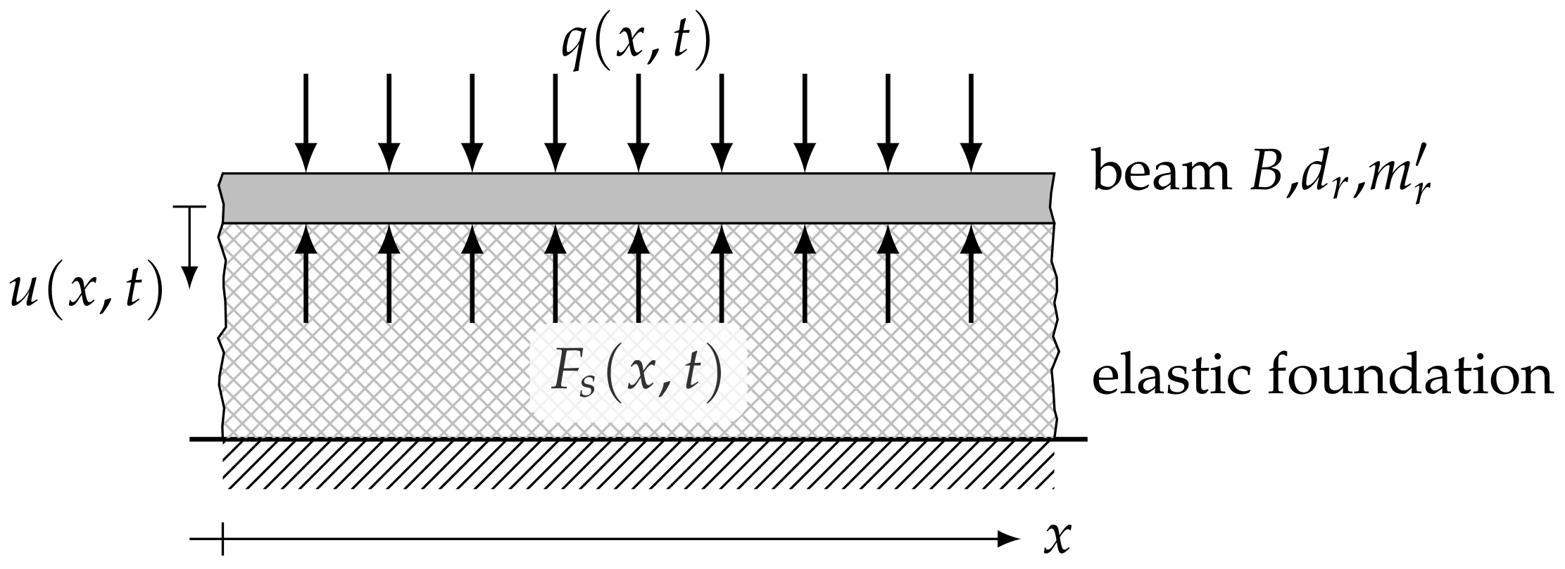
In the present paper, an infinite Euler–Bernoulli beam on an elastic foundation is considered, as shown in
Figure 1. While more sophisticated beam models, such as the Timoshenko beam, may generally be more appropriate in some cases, this simple model already serves the purpose of demonstrating the applicability of the FDM. The following differential equation describes the bending vibrations of the Euler–Bernoulli beam on an elastic foundation [
5,
26]:
The transverse deflection
u depends on both
x—the coordinate along the beam axis—and the time
t.
B is the bending stiffness, and
is the beam mass per unit length.
q represents the excitation force per unit length, and
is the viscous damping coefficient per unit length of the beam. The force
represents the effect of the foundation. Equation (
1) is a fourth-order partial differential equation, and its solutions correspond to bending waves on the beam. Because (
1) is just an approximation, its solutions may exhibit nonphysical behaviors. This is especially true for high frequencies, where the phase speed of the waves grows above every limit. This is a major challenge for the numerical treatment in the time domain. However, the same is also true for more sophisticated beam theories. As long as the bending wavelength is greater than six times the height of the beam, good agreement with more sophisticated beam theories can be obtained with the Euler–Bernoulli beam theory [
28].
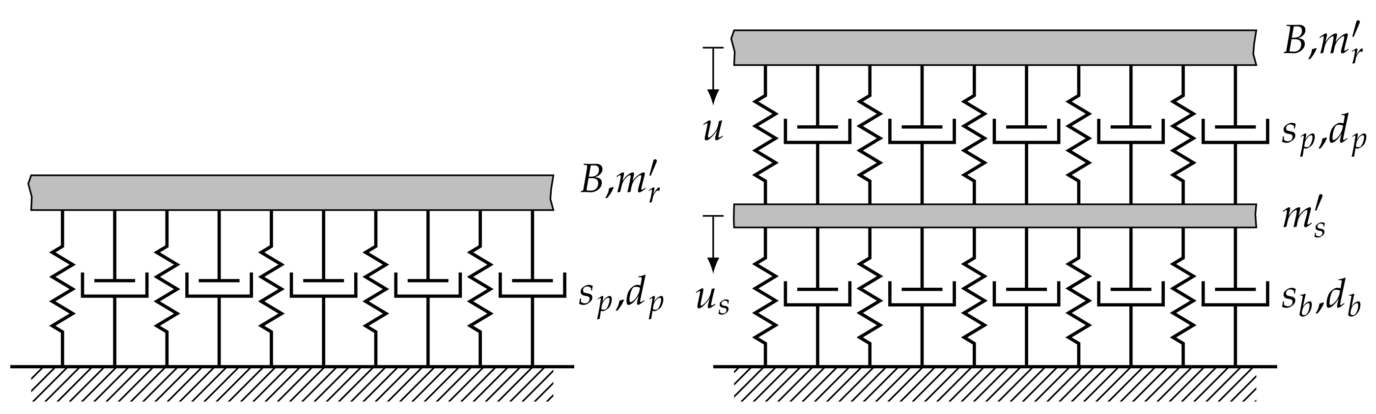
The effect of an elastic foundation (
Figure 2) can be modeled as
where
and
are the stiffness and the viscous damping coefficient per unit length, respectively, and
in the case of a single-layer elastic foundation. For a two-layer elastic foundation,
is the transverse deflection of the intermediate layer and is given by
with the mass per unit length
of the intermediate layer, the stiffness per unit length
, and the viscous damping coefficient per unit length
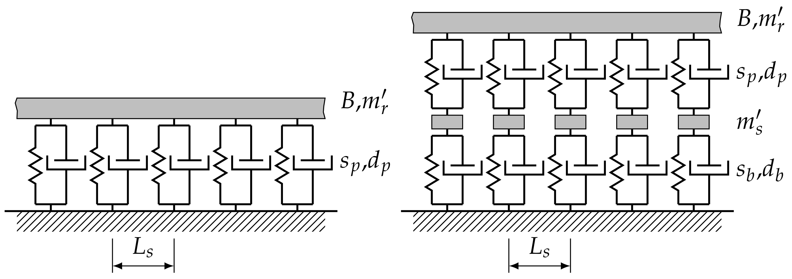
of the lower elastic layer. The viscous damping coefficients and stiffnesses per unit length may vary with the location. Whereas for continuously supported beams, they are constant along the length, discrete supports can be modeled by setting them to zero at all locations, except at the supports. This is illustrated in
Figure 3 for the case of equally spaced supports that are a distance
apart.
With the system of differential equations resulting from (
1)–(
3), the beam deflections can be calculated for both the single-layer and two-layer elastic foundation and continuous or discrete support. This analysis leads to some characteristic frequencies that determine the frequency response of these systems. For the single-layer supported beam, the frequency
corresponds to the resonance frequency of a spring–mass system when the mass of the beam per unit length is supported by the stiffness per unit length. This frequency is a cut-on frequency, as free wave propagation occurs only for frequencies above
. For frequencies well above this value, the wave propagation tends to be the same as that for an unsupported beam [
8].
For the two-layer support, two resonance frequencies are found. The frequency
characterizes the resonance of the mass of the intermediate layer on the stiffness
. An anti-resonance occurs at
. Cut-on frequencies also exist for the two-layer supports:
Below
, there is no wave propagation. For frequencies
, free wave propagation can be observed. A blocked region for
follows. For frequencies above
, the wave propagation also tends to that on an unsupported beam [
8].
In the frequency domain, damping effects are often considered by using a complex-valued stiffness
, where
is the damping loss factor, which is usually taken with no weak frequency dependence. In the time domain, however, it is not feasible to use complex-valued quantities. Therefore, the loss factor is converted into the viscous damping coefficient by using
Only for a monofrequent response at frequency
, the loss factor and the viscous damping coefficient result in fully identical damping effects [
8].
3. Finite Difference Method for Infinite Beams on Foundations
To determine the beam deflections
from (
1), (
2), and (
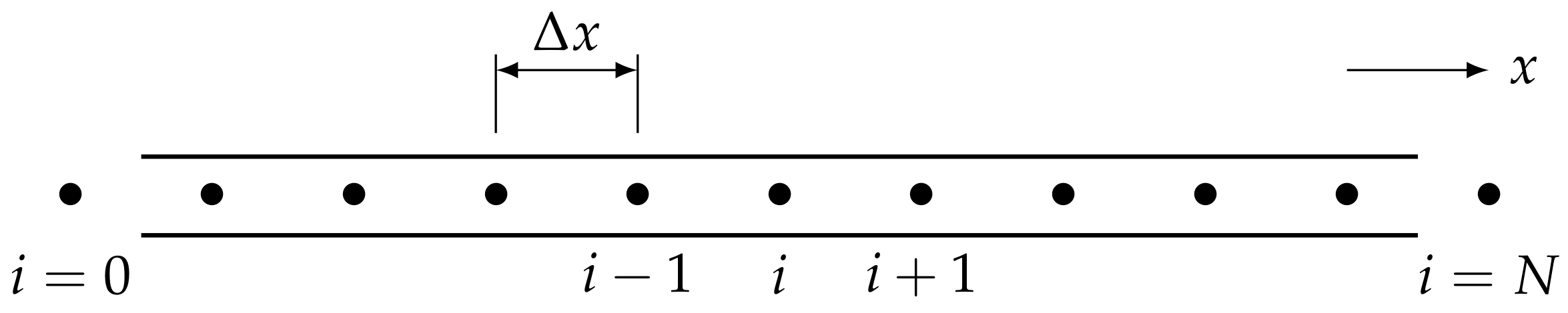
3) by using finite differences, the beam needs to be discretized into
N equally long segments. The number of nodes is
with a local step size
, as shown in
Figure 4. The time is also discretized into discrete intervals
. Hence, the solution domain
is covered with a rectangular grid with uniform spacing
and uniform spacing
.
Equations (
1) and (
2) can be rewritten as
This equation contains a fourth derivative in space, as well as first and second derivatives with respect to time. In the FDM, these derivatives are approximated using finite differences (an overview of the FDM is available in [
29]). For the fourth derivative in space in (
7), this yields [
24]
Here and in the following, the lower indices denote the numbers of the grid points such that
. In the matrix representation, (
8) can be rewritten as
with the
pentadiagonal matrix and the
vector
respectively. The time derivatives can be approximated in a similar fashion:
In this notation, the upper indices define the time step such that .
There are various possible approaches to solving the finite difference version of (
7), where all derivatives are replaced by (
9), (
11), and (
12). In this paper, the implicit Crank–Nicolson scheme was chosen because it has been shown that it yields stable solutions for the Euler–Bernoulli beam wave equation and positive values of
B and
[
24,
26]. The general idea of the Crank–Nicolson scheme is to replace all parts except the time derivatives at instant
n with a weighted sum of its values at different instants. Thus, an implicit formulation arises where a system of equations has to be solved to produce the values of
u at the next instant [
30]. In the present case, these terms on the right-hand side of (
7) are evaluated at instants
and
, which leads to
, and
indicate the stiffness and damping per unit length at node
i.
describes the force per unit length at the node
i at time step
n. The separation of time steps
,
n, and
results in the implicit representation of (
7):
which allows the computation of the result for instant
from the values in the past at instants
n.
For a two-layer elastic foundation, the finite difference version of (
3) is needed in an implicit numerical form as well:
where
and
indicate the stiffness and damping coefficient per unit length of the intermediate layer at the node
i, respectively.
To solve both (
14) and (
15) together for any grid point
i, it is useful to join them into one system of equations:
The sub-matrices contained here can be found in
Appendix A. Note that all sub-matrices are diagonal, except
and
, which are pentadiagonal. This is an advantageous property for the quick solution of (
16). The support mass deflection
and the force per unit length
are, respectively, in vector form, equivalent to
in (
10). For a beam with a single-layer support, only (
14) is necessary, omitting all terms containing
. Generally, all stiffness and damping values may be updated after each time step, depending on the deflection history up until that time step. This would enable the modeling of nonlinear behavior of the foundation. A similar technique could be implemented for a nonlinear force excitation. However, in the following analysis, it is assumed that both foundation and excitation exhibit strictly linear behavior.
For the solution procedure of the FDM, it can be assumed that at the outset, the deflection and its time derivative (the velocity) along the beam are given. With these initial conditions, the unknown deflections of time step
can be calculated. In this way, it is possible to solve (
16) for each forthcoming time step.
Given the grid spacing in space and time, a characteristic value
can be defined for the present analysis. For a spacing
that is too small, oscillations of the solution can occur even with the implicit FDM because the Crank–Nicolson scheme is not L-stable. The Crank–Nicolson scheme for parabolic difference equations has a good numerical accuracy only for small values of
r (
) [
31]. Therefore, the spatial spacing of the grid is related to the time step:
The constant b must be valid ().
One problem with the application of the finite difference method to infinite systems is that an infinite number of grid points N would be required. Therefore, methods have to be developed to mimic the infinite properties of the beam with a finite number of grid points. One possible approach is to equip the boundaries of a finite system in a way in which all wave energy is absorbed once it travels toward the boundaries. Artificially increased damping near the boundaries is a possible method for accomplishing this. This damping absorbs the energy of the bending wave in such a way that virtually no part of the wave is reflected from the boundaries.
Since there should be no deflections at the boundaries (
/
), no specific precaution for the formulation of a boundary condition needs to be taken in
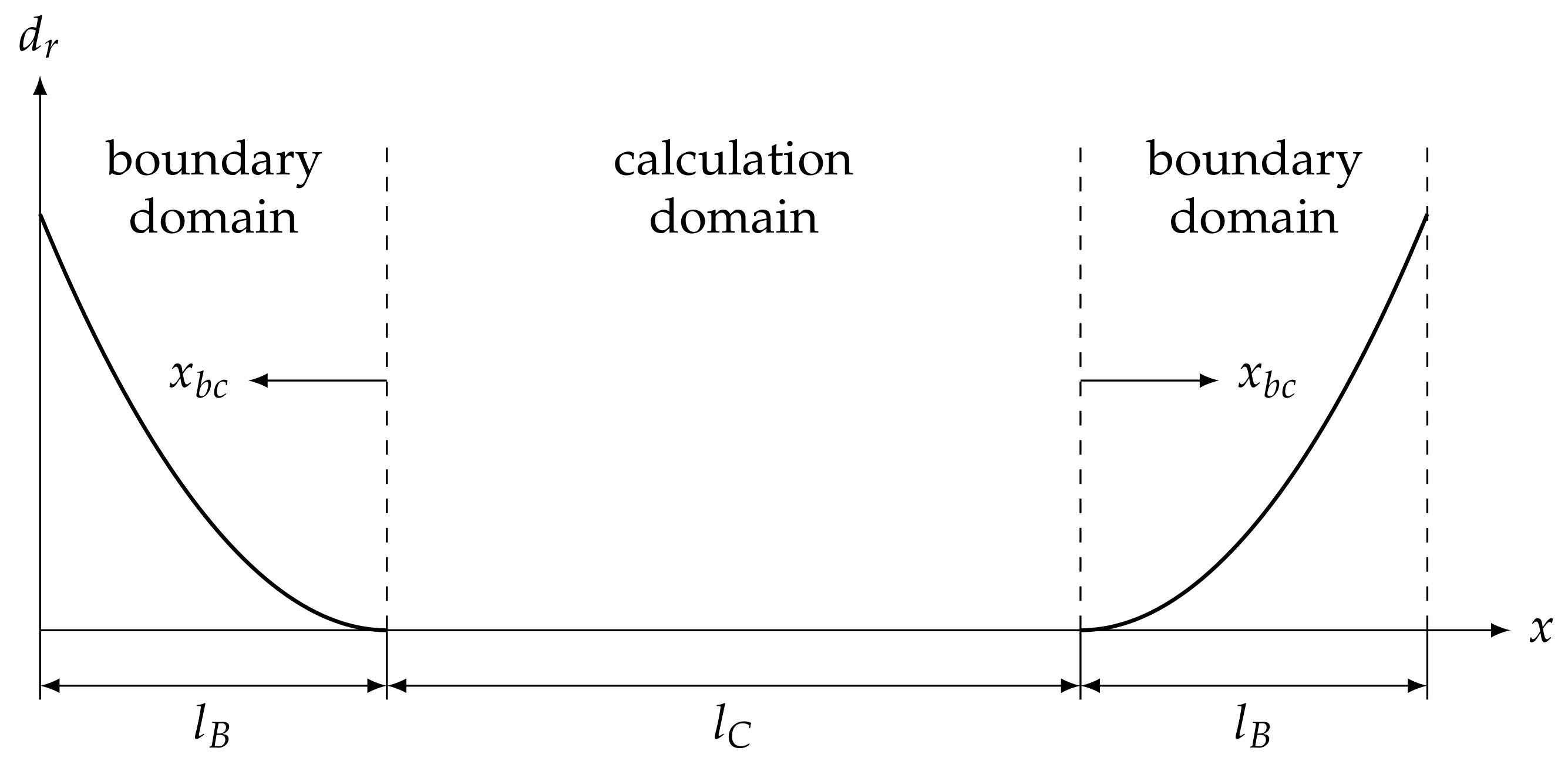
. To apply the damping, the spatial domain is divided into boundary domains and a calculation domain; see
Figure 5. In the boundary domains, the inner damping coefficient
increases slowly towards the boundaries over the length
. To ensure that the damping of the boundary connects fluently to the damping of the computational domain without a leap, a function is needed whose derivative disappears when it equals zero. Therefore, functions of the form
were chosen with exponents
.
is the coordinate of the boundary domains and
,
is the number of grid points used for the boundary domains (see
Figure 5).
is the maximum value of the damping coefficient in the boundary domains.
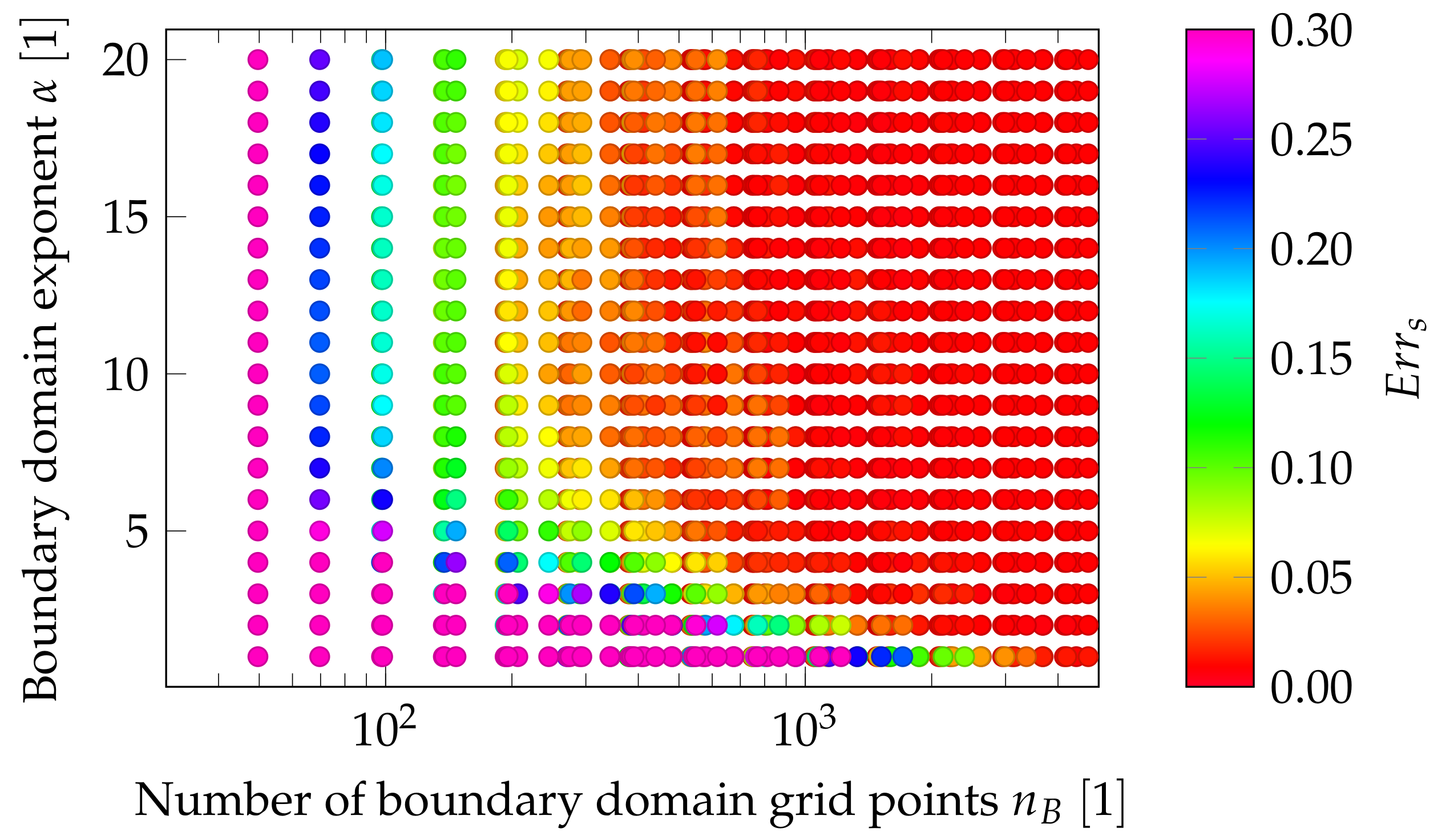
The parameters
,
, and
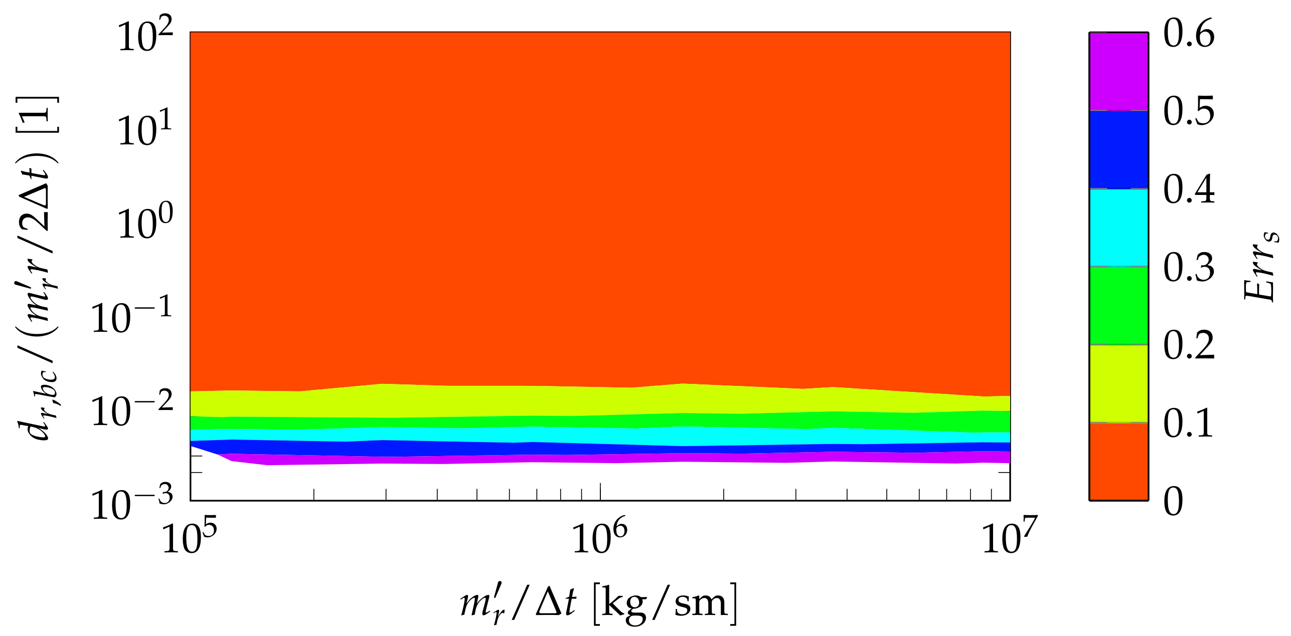
should be defined to accurately simulate the properties of an infinite beam while requiring less computing time. Therefore,
should be as small as possible because, otherwise, the increases in the grid size
N result in greater lengths of computing time. Therefore, a parametric study was conducted to determine these parameters. The parametric study revealed that the exponent
should be larger than 7 to obtain low values of
(
Figure A1). With the approach
, good simulations of the infinite beam can be obtained over a wide range of different
and, thus, different sound propagation velocities; see
Figure A2.
If the analysis is carried out for a time interval
, in principle, the result allows the consideration of frequency components down to
For other finite difference models of wave propagation, it was found that accurate solutions were obtained with
, where
was the wavelength [
32]. Considering
as the shortest bending wavelength of interest of a free infinite Euler–Bernoulli beam, the upper frequency limit determined by the spatial distance is given by:
In the present analysis, sufficiently precise solutions were already found with the constant
. Inserting Equation (
17) into Equation (
20) yields
The upper frequency limit is also directly dependent on b. The constant b should preferably be set at the lowest possible value () for a broad frequency range, but this also increases the computational time.
The amplitude of the deflection is well approximated at high frequencies with 10 time steps per period. This results in the following upper frequency limit determined through time sampling:
The lower frequency of Equation (
21) or Equation (
23) indicates the maximum frequency for the calculation procedure. Which of these two frequencies determines the upper limit depends on the choice of
b and
g.
4. Results and Discussion
In the following, the applicability of the proposed FDM procedure to rail-like applications is examined. Different beam models are set up by using the parameters given in
Table 1; these can be taken as representative for a railway rail; see [
8] (Chap. 3). Unless otherwise specified, the FDM models all use the parameters from
Table 2. The overall length of the calculation domain is 80 m, and both boundary domains are chosen to have a length of 36.5 m, which results in an overall length of the rail of 153 m.
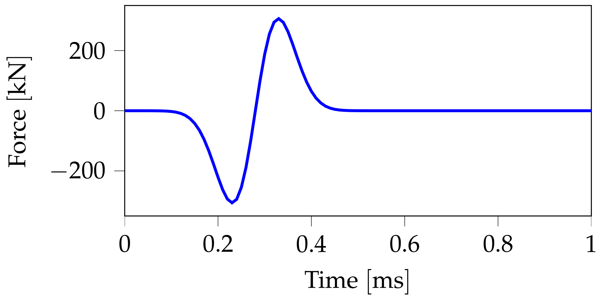
To investigate the propagation of bending waves in time and space, a broadband transient excitation was used. A pulse (first derivative of the Gaussian function) served as the force excitation
, which excited the beam at a fixed location
in the calculation domain (
Figure 6):
The arbitrary parameters a and govern the amplitude and duration of the pulse, respectively. is the Dirac delta.
In the case of a discretely supported beam with two layers, the computation required half a minute of CPU time on an Intel® Core™i5-7200U CPU at 2.50 GHz for time steps.
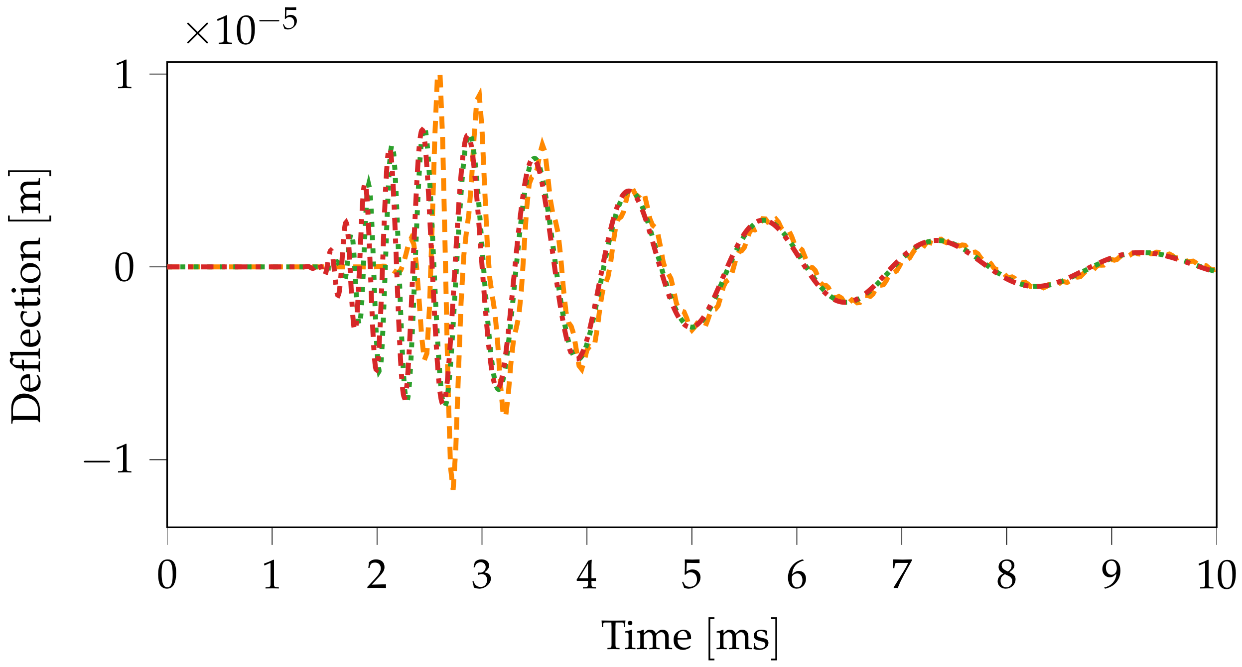
Figure 7 shows the response of a beam on a single-layer elastic foundation at a distance of 10 m from the excitation point. The result is given for different time step sizes and associated spatial step sizes according to (
17). The expected dispersive behavior of the bending wave can be observed. The high-frequency components and, thus, smaller wavelengths propagated faster than lower-frequency components. Therefore, bending waves with small wavelengths passed the receiver point
first. Over time, the wavelengths increased. From the results, it turned out that with a smaller time step size (and smaller spatial step sizes), shorter-wavelength components could be computed more accurately. These short-wavelength components traveled faster due to the dispersion. Therefore, the first high-frequency wave components for a time step size of
s occurred earlier than those for the other, larger time step sizes. The energy originally introduced by the pulse was distributed over a larger frequency range for the smaller time step size than for the larger time step sizes. This explains why the maximum amplitudes were somewhat larger for the larger time steps. However, for lower-frequency components (and, thus, at a later time), the results are very similar to each other.
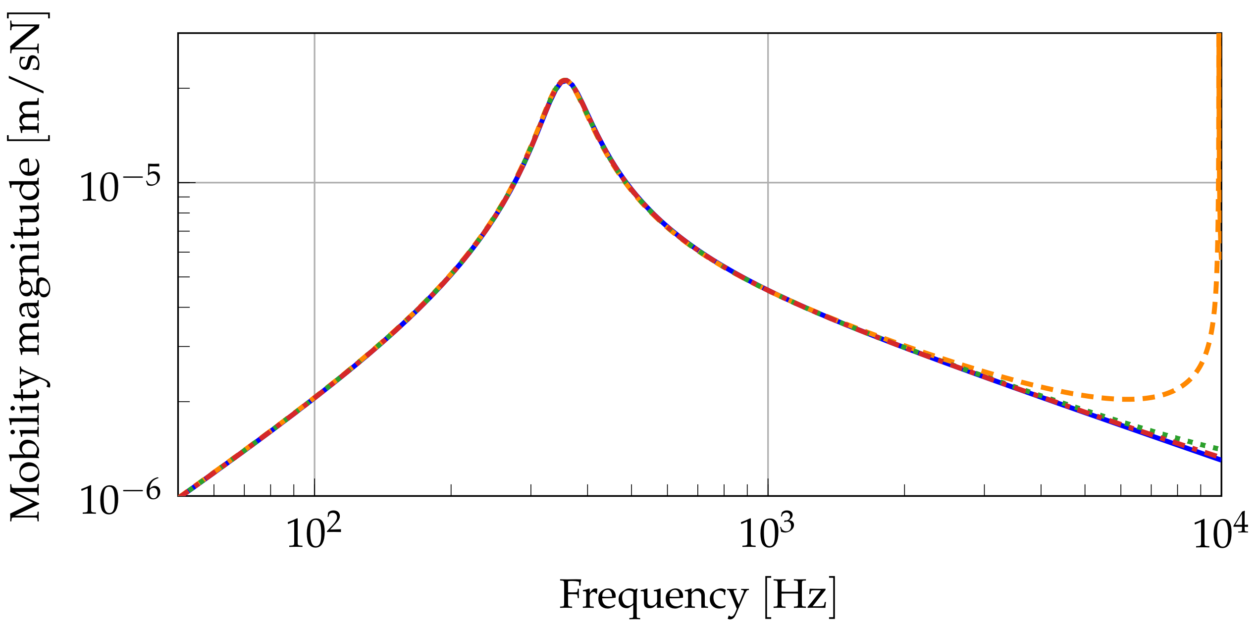
From a frequency-domain perspective, it would be interesting to know to the upper frequency at which a model produces reliable results. Analytical models are available that allow for a comparison. For a continuously supported beam on single-layer elastic foundation, the mobility
is given by [
8]
where
is the distance from the force point and
is the bending wave number.
Figure 8 shows the results for the point mobility (
) at the excitation point as a function of frequency. To compute any mobility using the FDM method, the beam is excited at one point (
24), and the response of the beam at one or more receiving points is computed. The response and the excitation signal are then transformed using a discrete Fourier transform. The mobility is estimated from the Fourier transforms
and
using
For each time step size, the upper frequency limits could be estimated using (
23).
Figure 8 shows that for
s, the deviation from the analytical benchmark increased rapidly above the maximum frequency of 4 kHz. However, for shorter time step sizes and the associated smaller spatial step sizes, a much better agreement with the analytical solution could be observed. Since a time step size of
s gave satisfactory results in the frequency range of interest, this step size was used for all remaining computations.
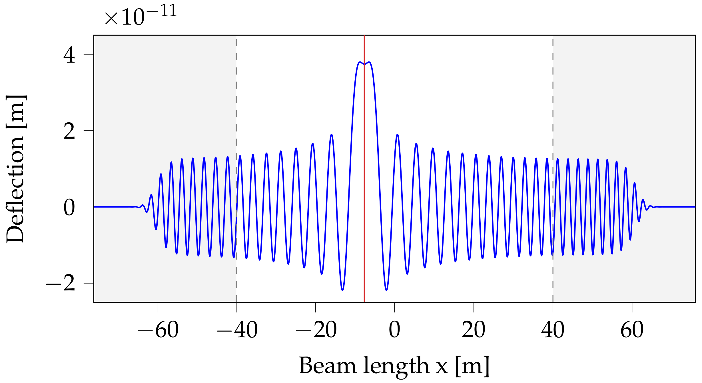
Figure 9 shows the deflection of the beam after 0.05 s. The dispersive propagation that is visible in
Figure 7 is superposed here by the resonance of the support. The decrease in the deflection amplitude in the boundary domain is obvious. As intended, the wave was damped and no reflection occurred.
To quantitatively analyze the effect of the proposed damped boundary domain method, the point mobility of an undamped, unsupported infinite beam was considered. It was given by [
28]
where
is the bending wave number.
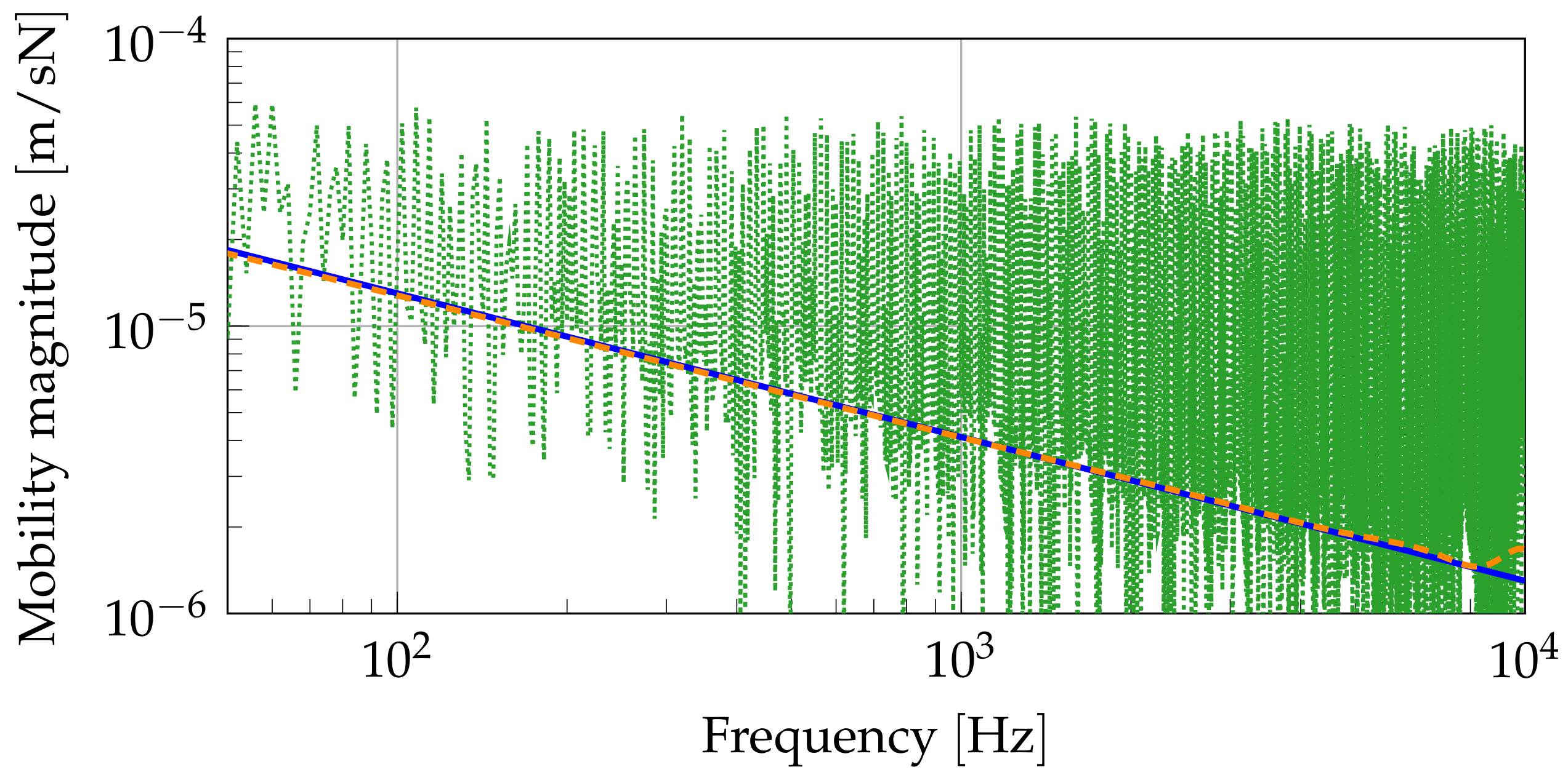
Figure 10 compares this result to that from the FDM if no boundary domain is used and to that of the FDM with a damped boundary domain. Without boundary domains, the beam was effectively finite, and thus, the eigenfrequencies and corresponding bending mode shapes governed the results. With the proposed boundary domains, the results were identical to the analytical results, except for some small deviations for very low and very high frequencies.
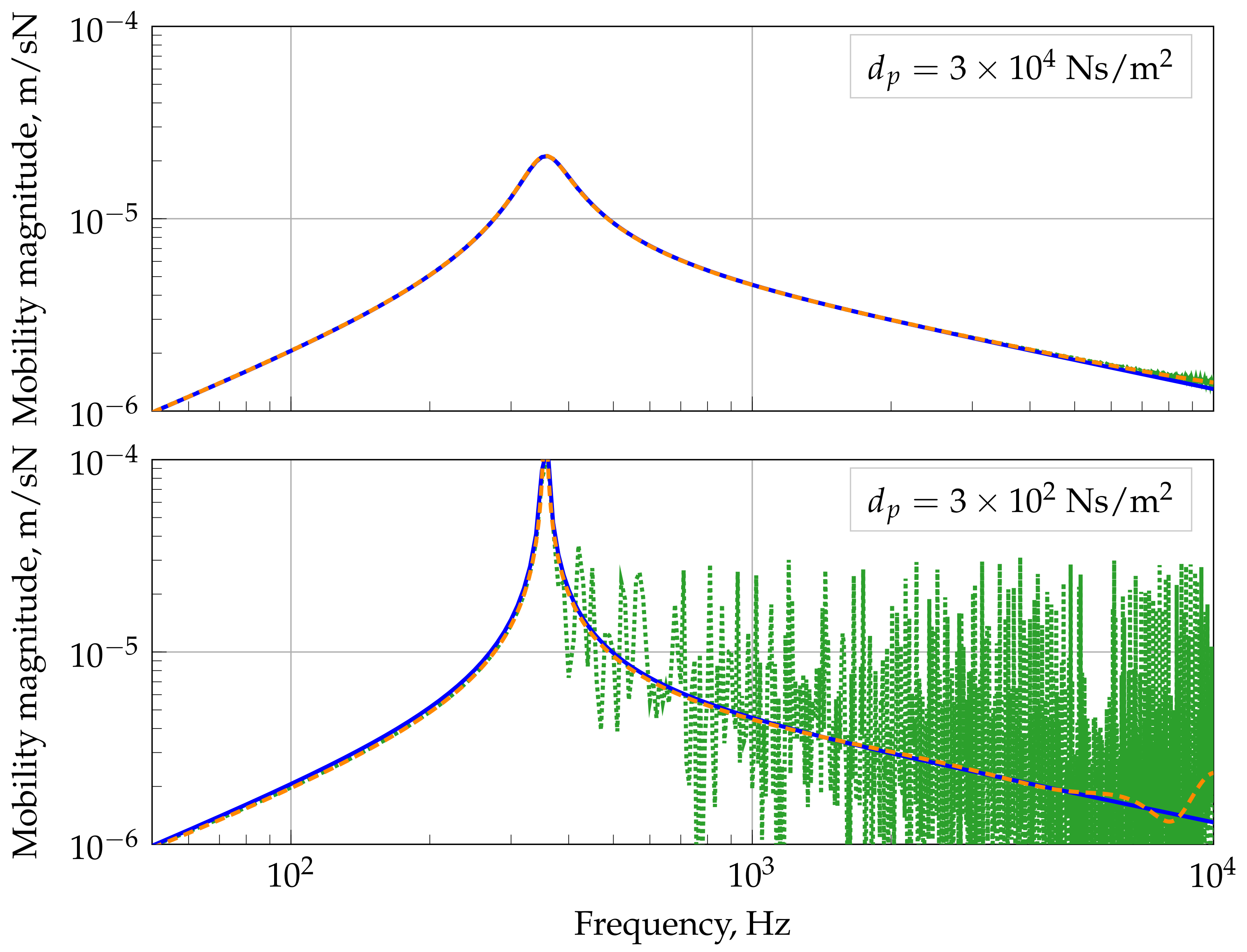
Figure 11 shows further results for the effects of the boundary domains, but for a continuously supported beam. Two cases were compared with different damping in the elastic foundation. If the damping was high, the boundary domains had less of an effect. With low damping and no boundary domains, the influence from modal behavior was essential, but only above the cut-on frequency
. Below the cut-on frequency, there was no modal behavior, since there was no free wave propagation.
The use of the damped boundary domains led to high agreement with the analytical results. Especially for weakly damped systems, they are essential.
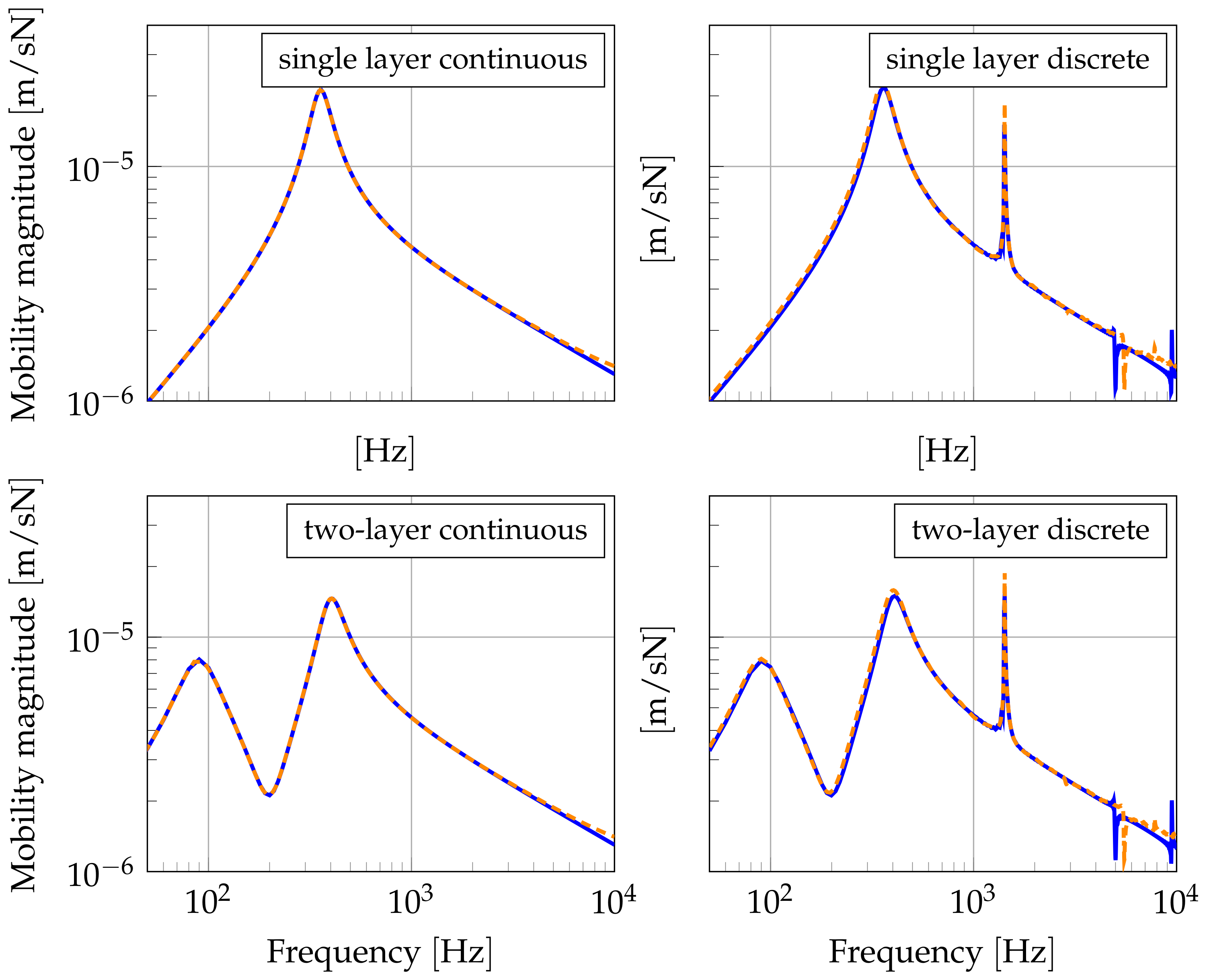
The last step in the validation of the FDM results was a comparison of the mobilities with analytical solutions for all four foundations types. While (
25) gives the mobility in the case of a single-layer continuous foundation, the analytical results for a continuous two-layer support beam are given by [
8]
where
and
. The length
is again the distance to the excitation point. An analytical method for the mobilities in the case of discrete supports is given in [
3] for the Euler–Bernoulli beam. The results from this model were used as benchmark for the FDM here.
The point mobility gives the response at the excitation point and is important for the characterization of the structure-borne sound excitation. Numerical and analytical results for the point mobility are shown in
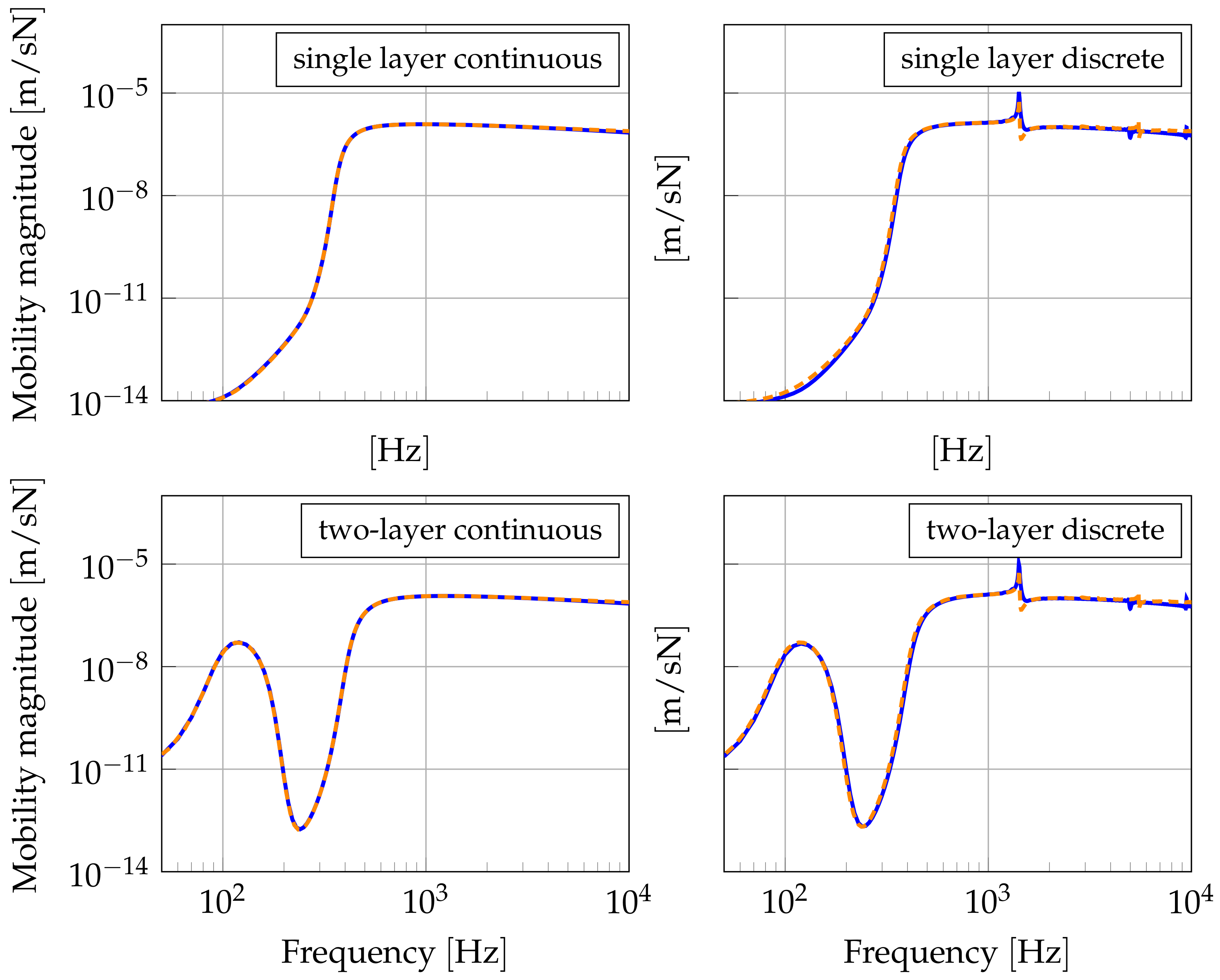
Figure 12. The propagation of structure-borne sound is more appropriately described by the transfer mobility, which relates the response at a location other than the excitation point to the excitation force. The results in
Figure 13 show the transfer mobility for a point at a distance of 10 m from the force point. In the case of discrete support, the excitation point is located in the middle between the two supports.
The FDM results for both the point and the transfer mobility agreed very well with the analytical results in all cases. The resonance frequency for the single-layer support given by (
4) at 356 Hz showed itself clearly in the results for the point mobility in
Figure 12. The same was true for the anti-resonance
at 201 Hz for the two-layer cases. The resonance
at 100 Hz was not noticeable due to the stronger influence of the cut-on frequency
at 90 Hz. For the two-layer support, the stop bands below
and between
and
at 400 Hz showed themselves in the significantly lower transfer mobility (
Figure 13).
The discretely supported beams exhibited a sharp peak for the pinned–pinned frequency at 1414 Hz, which was approximately the frequency corresponding to half of the bending wavelength of the distance between the supports. This frequency was also accurately predicted with the FDM. Only for higher frequencies that were well above the frequency range of interest in rolling noise models could minor differences from the analytical solution from [
3] be found.


 s ( m, kHz),
  s ( m, kHz),
  s ( m, kHz).
 Analytical mobility (Equation (25)),
  s ( m, kHz),
  s ( m, kHz),
  s ( m, kHz).

 Analytical mobility (28),
  with boundary domains,
  without boundary domains.
 Analytical mobility (25),
  with boundary domains, external/export
  without boundary domains.
 Analytical results,
  finite difference method results.

 Analytical results,
  finite difference method results.
