Figure 1.
Control system outlook.
Figure 1.
Control system outlook.
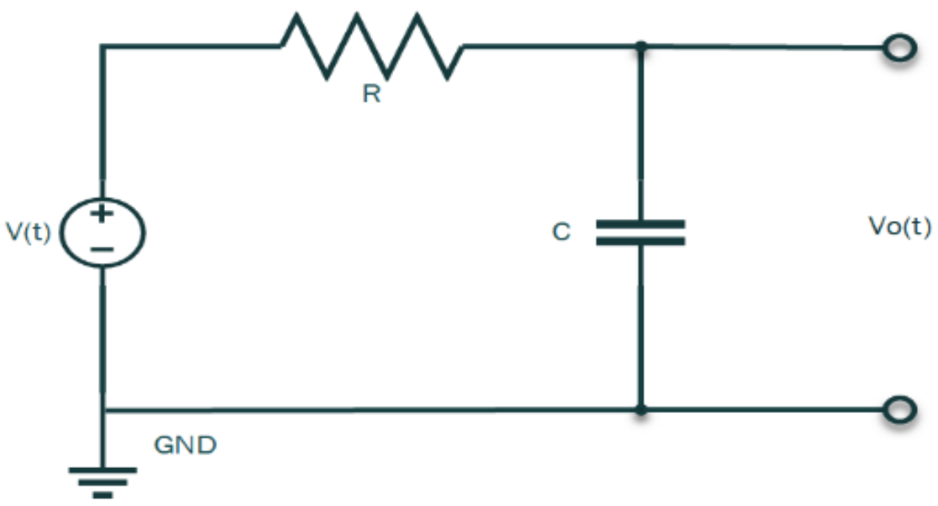
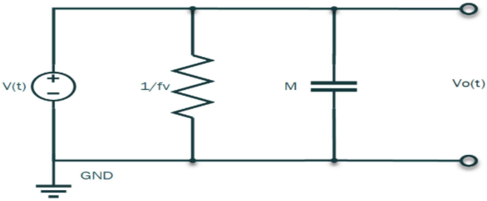
Figure 2.
I-P transducer time-domain network circuit.
Figure 2.
I-P transducer time-domain network circuit.
Figure 3.
I-P transducer s-domain network circuit.
Figure 3.
I-P transducer s-domain network circuit.
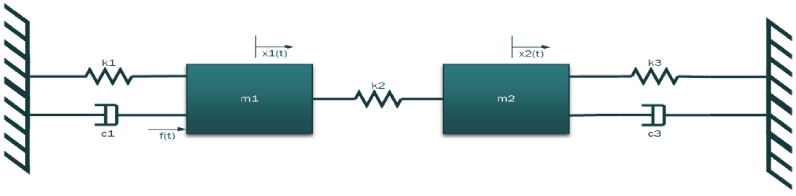
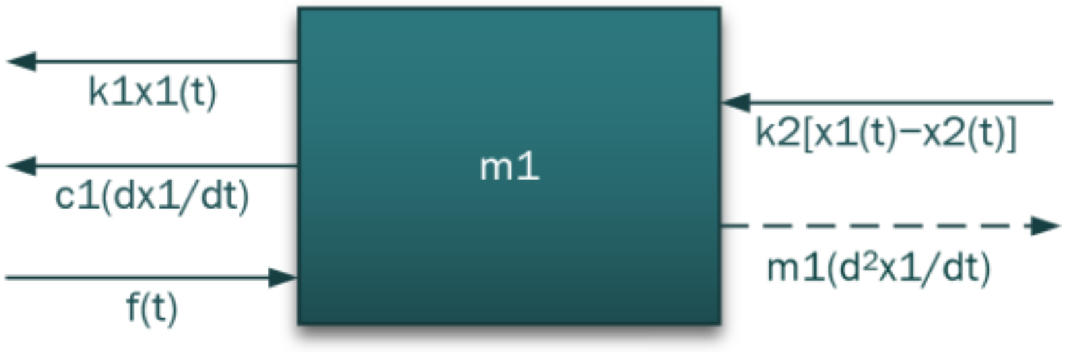
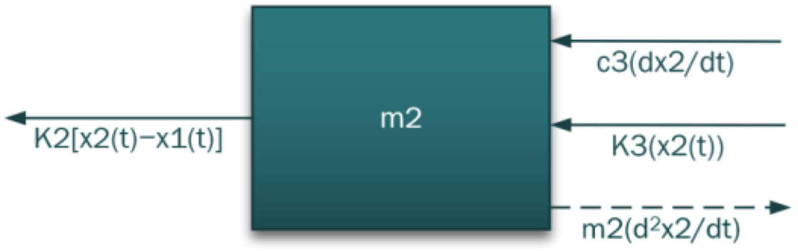
Figure 4.
Second DOF mass spring damper system (spring and diaphragm valve and sonic horn).
Figure 4.
Second DOF mass spring damper system (spring and diaphragm valve and sonic horn).
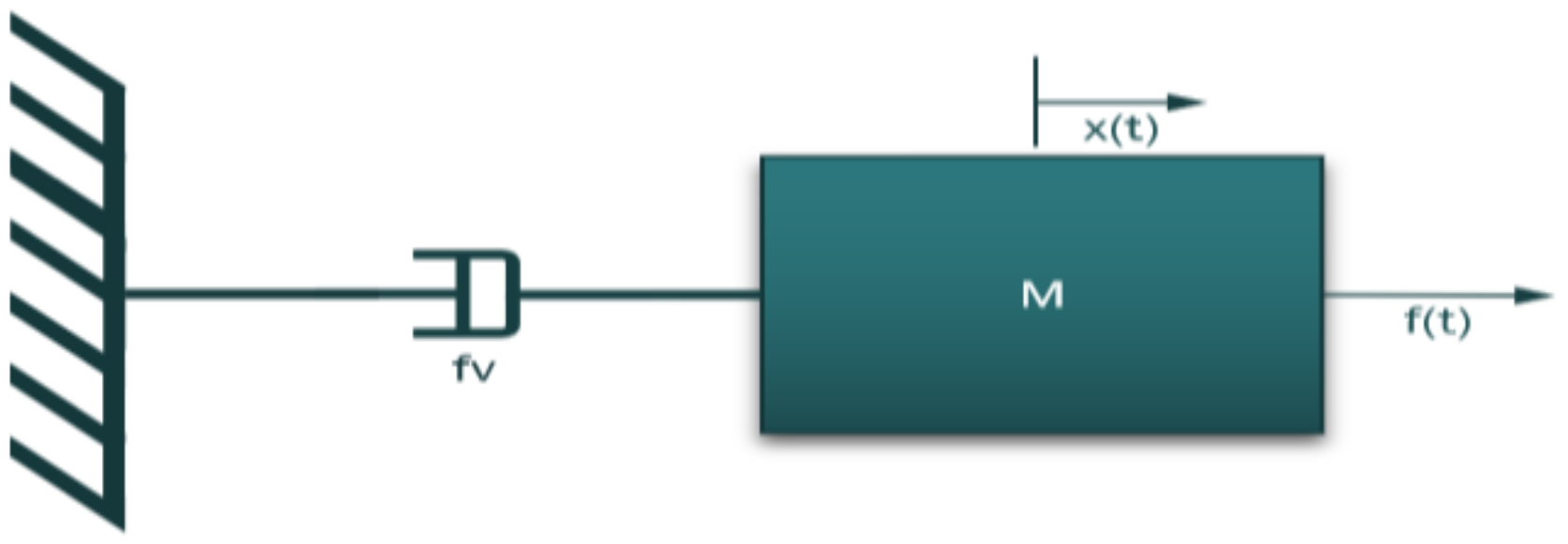
Figure 7.
Piezoelectric pressure sensor 1 DOF mass damper system.
Figure 7.
Piezoelectric pressure sensor 1 DOF mass damper system.
Figure 8.
Parallel analogous circuit (time-domain).
Figure 8.
Parallel analogous circuit (time-domain).
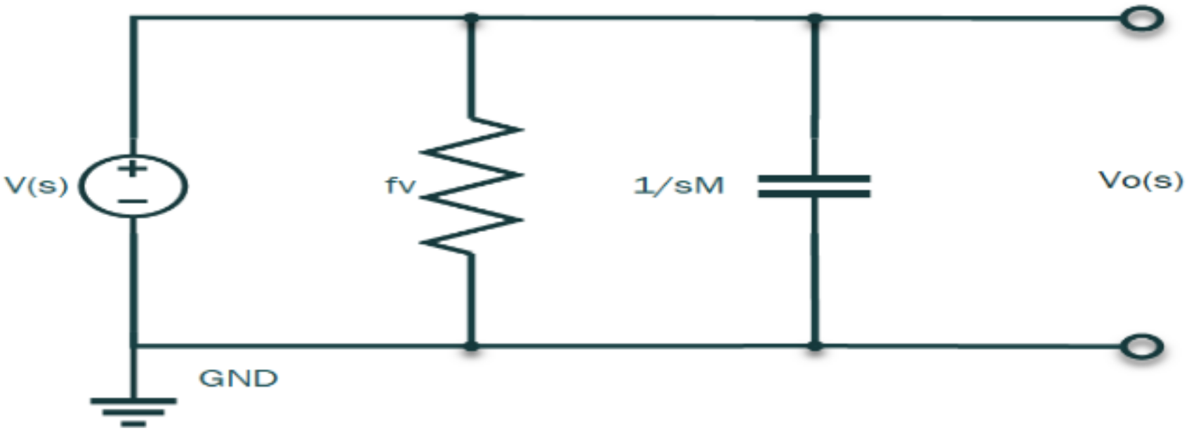
Figure 9.
Piezoelectric pressure sensor Laplace transformed parallel analogous circuit.
Figure 9.
Piezoelectric pressure sensor Laplace transformed parallel analogous circuit.
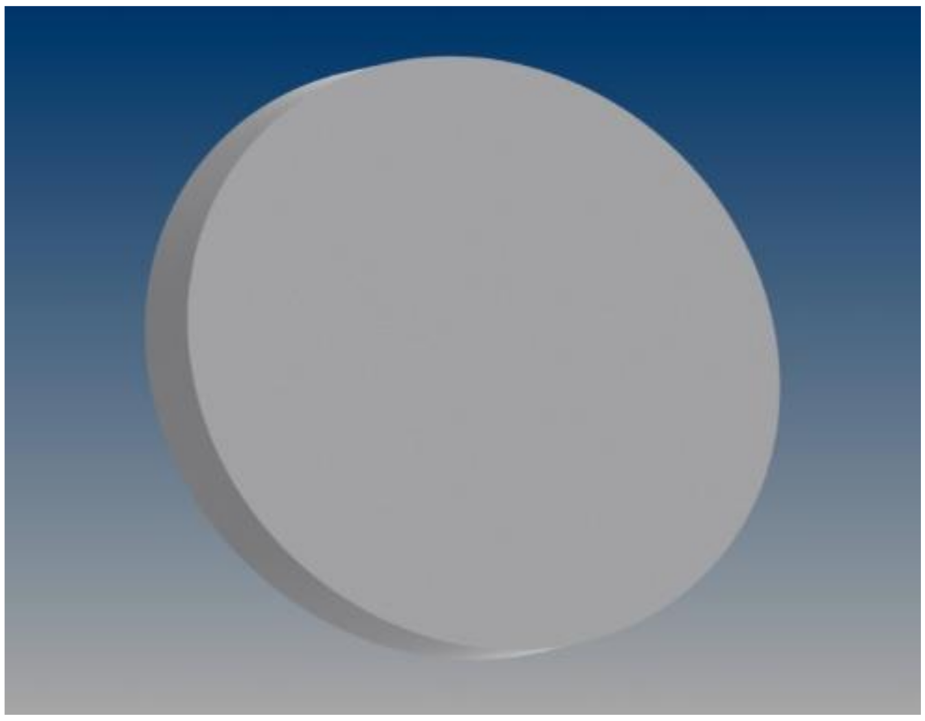
Figure 10.
Silicon nitride diaphragm.
Figure 10.
Silicon nitride diaphragm.
Figure 11.
Titanium diaphragm.
Figure 11.
Titanium diaphragm.
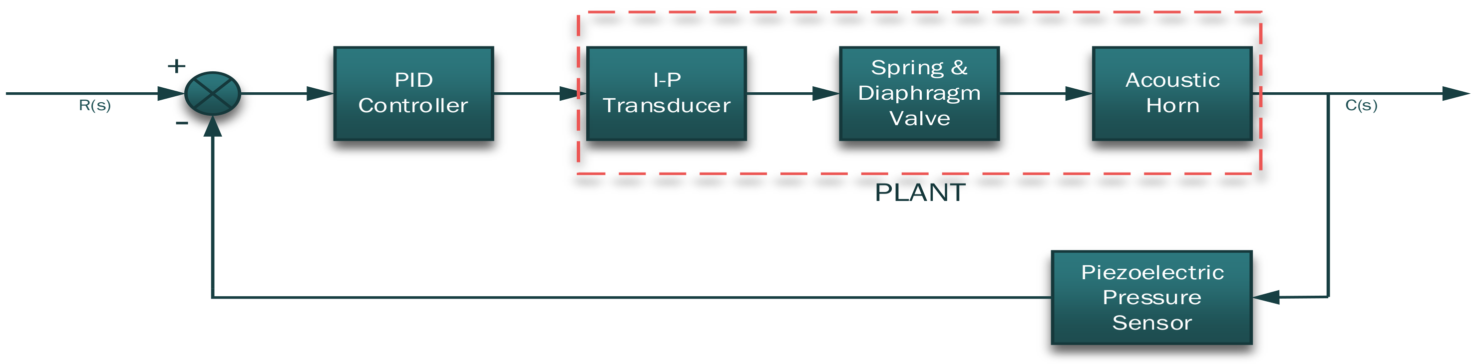
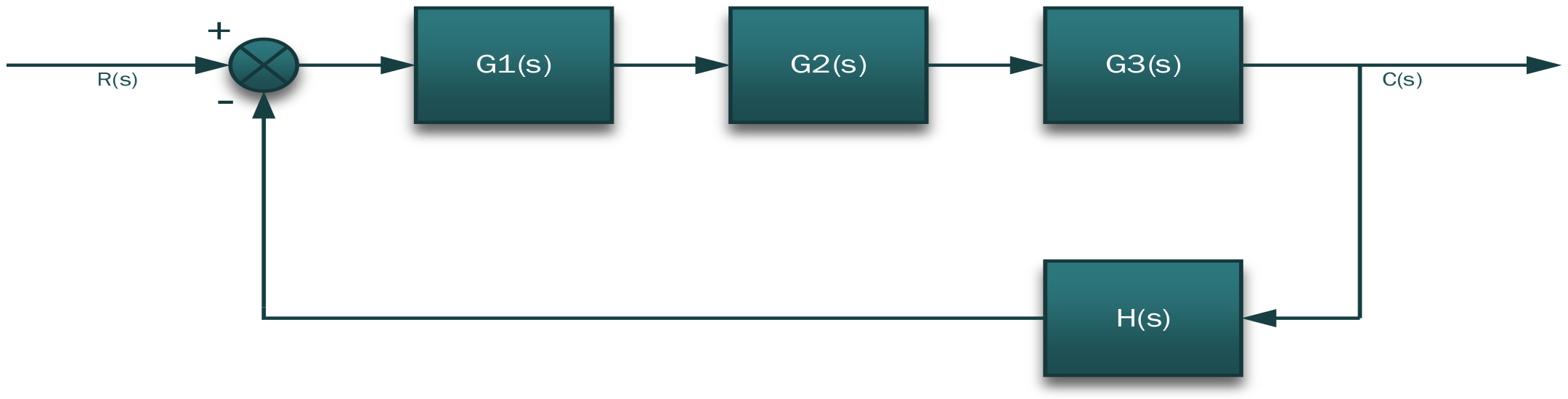
Figure 12.
System block diagram.
Figure 12.
System block diagram.
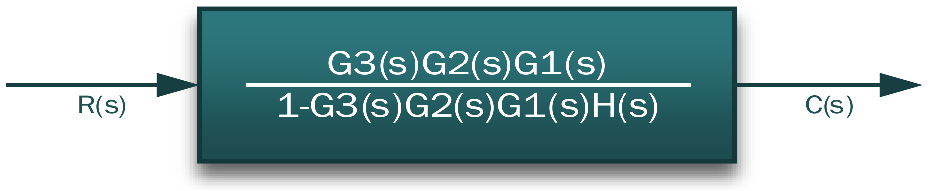
Figure 13.
Equivalent control system transfer function Finalsys.
Figure 13.
Equivalent control system transfer function Finalsys.
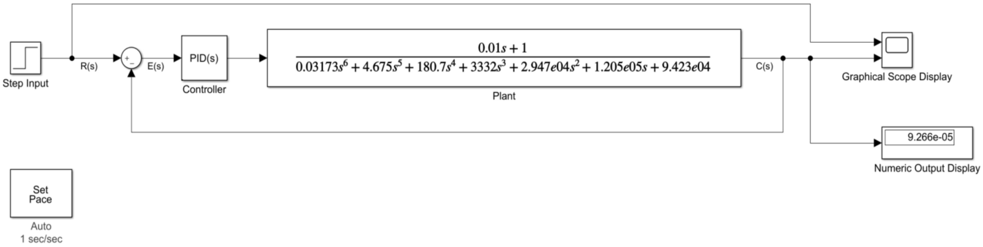
Figure 14.
Closed-loop system configuration.
Figure 14.
Closed-loop system configuration.
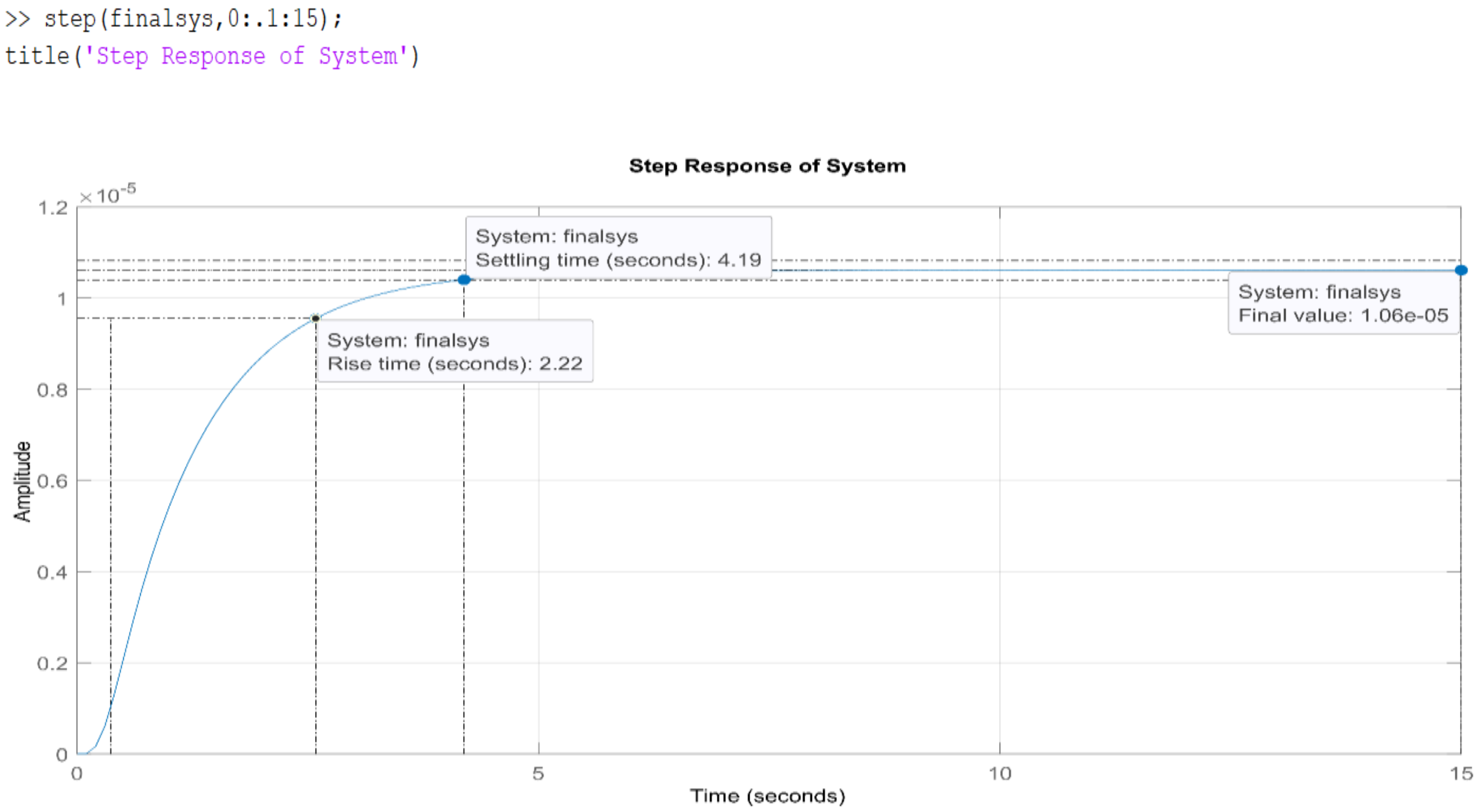
Figure 15.
Finalsys step response.
Figure 15.
Finalsys step response.
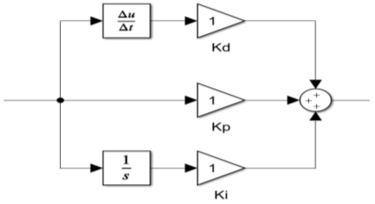
Figure 16.
PID controller block expanded view [
22].
Figure 16.
PID controller block expanded view [
22].
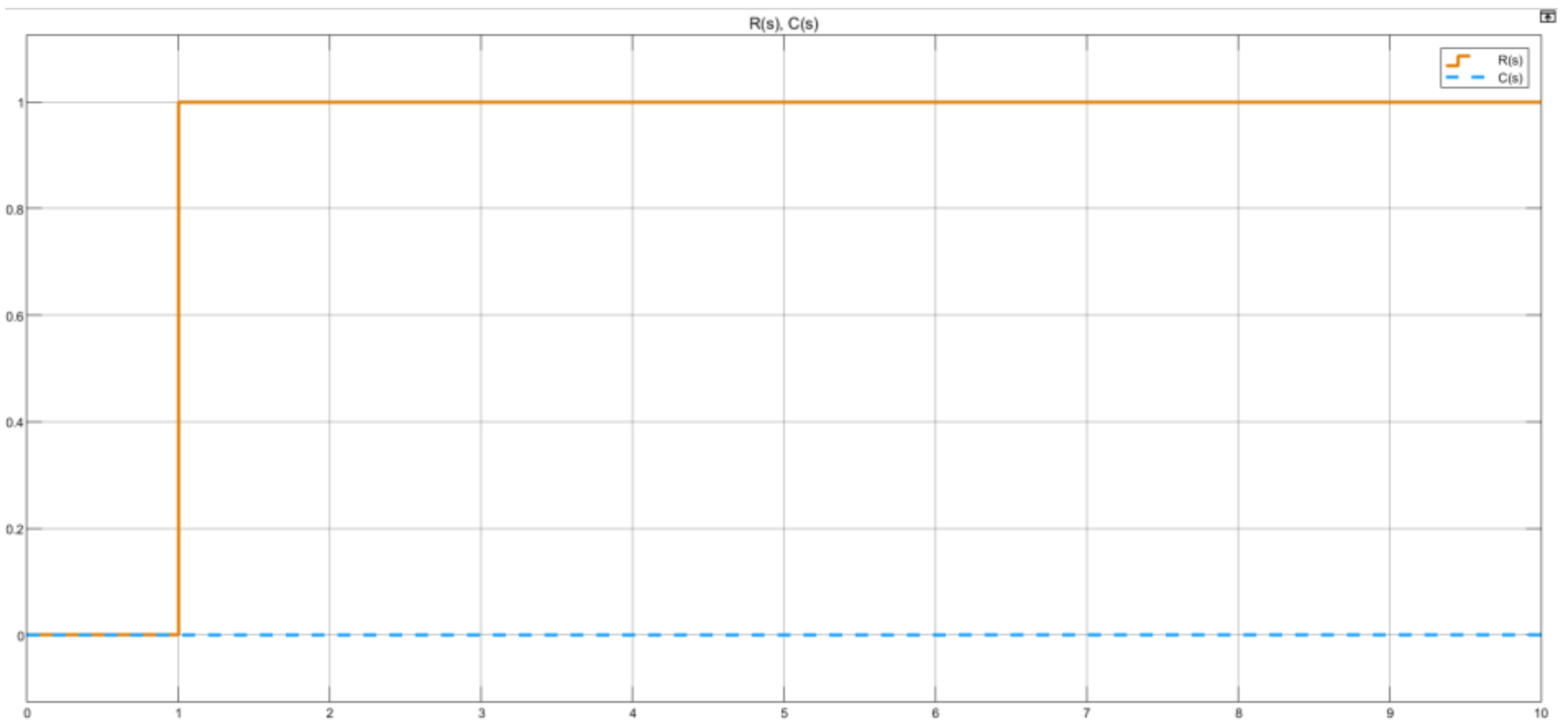
Figure 17.
Untuned system reference tracking plot.
Figure 17.
Untuned system reference tracking plot.
Figure 18.
Untuned system output demonstration.
Figure 18.
Untuned system output demonstration.
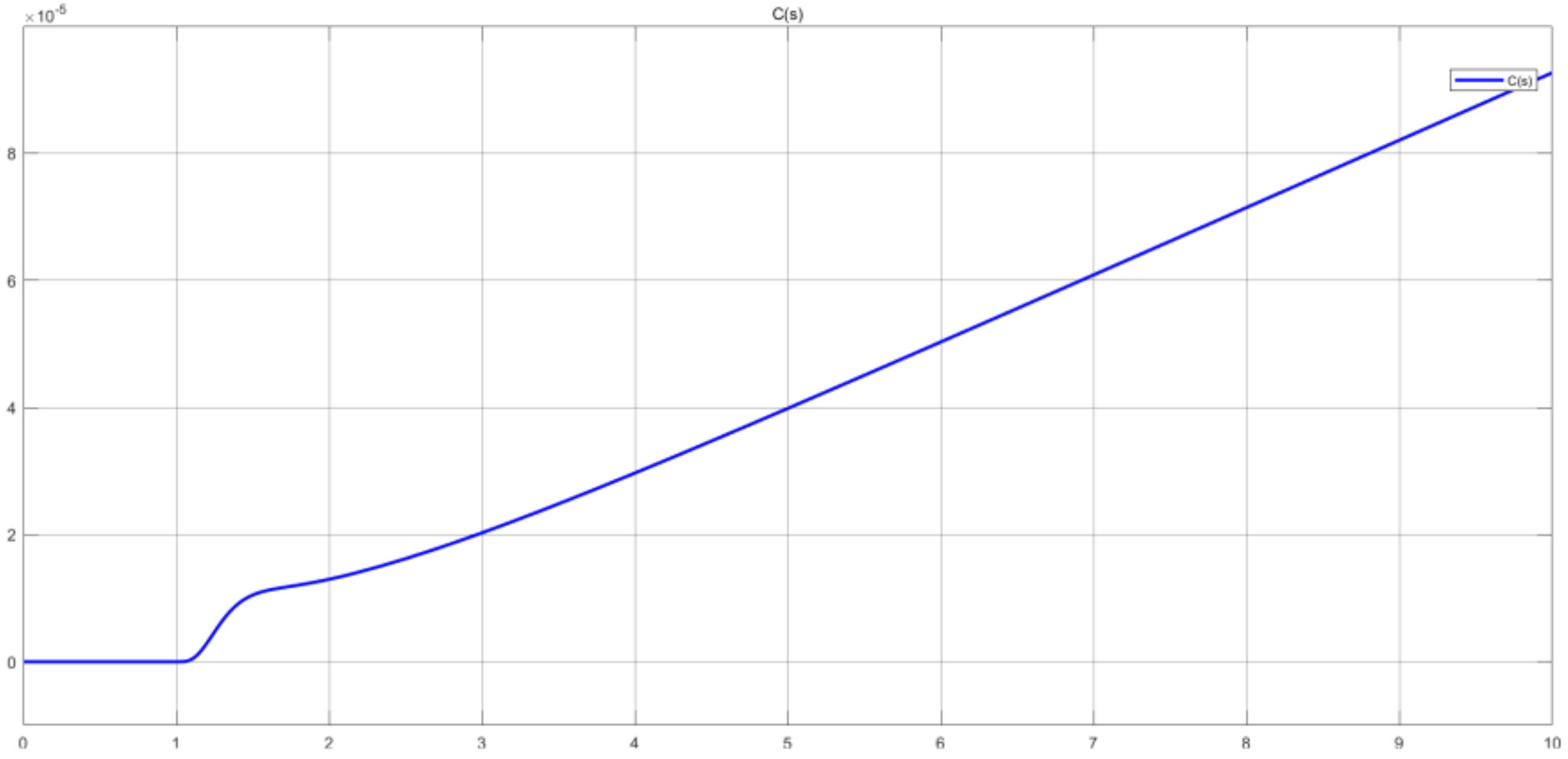
Figure 19.
Untuned system C(s) signal.
Figure 19.
Untuned system C(s) signal.
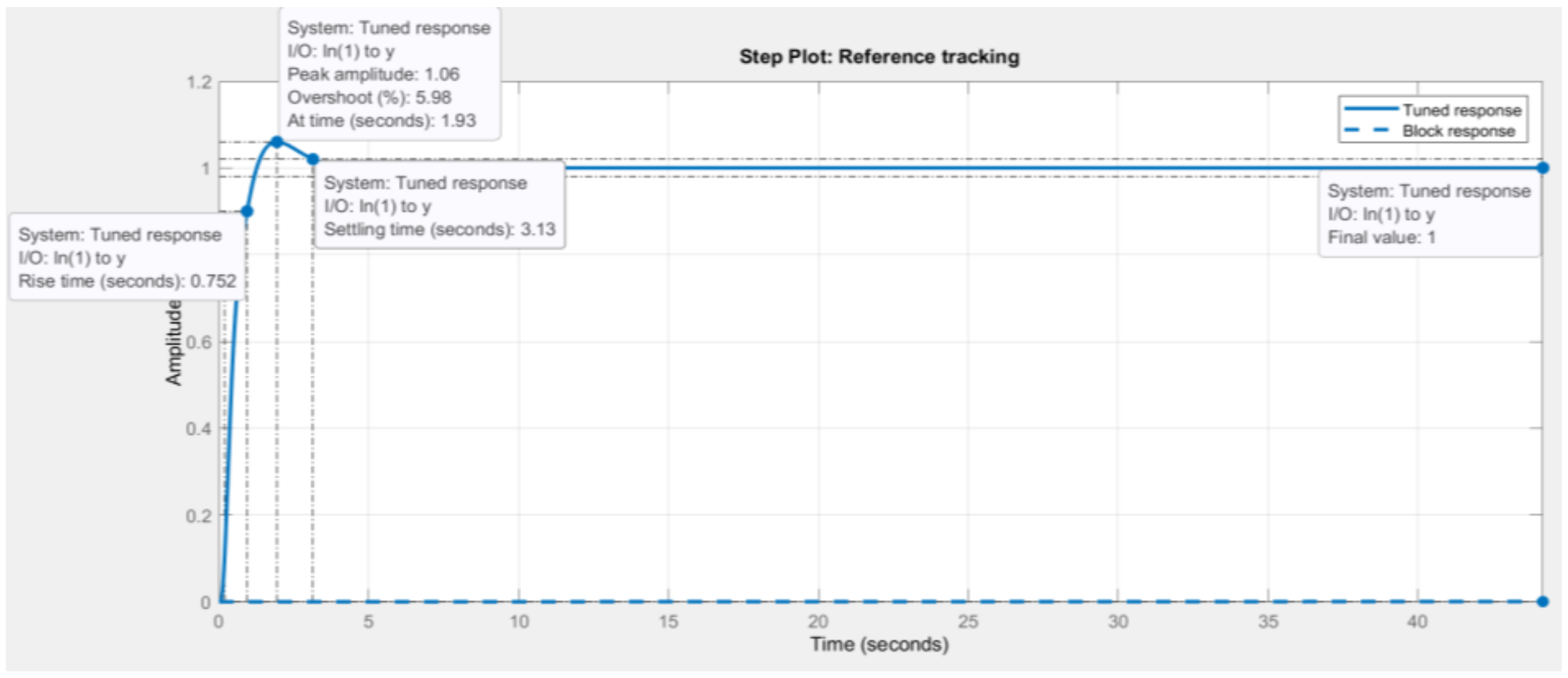
Figure 20.
Tuned system response (reference tracking focus).
Figure 20.
Tuned system response (reference tracking focus).
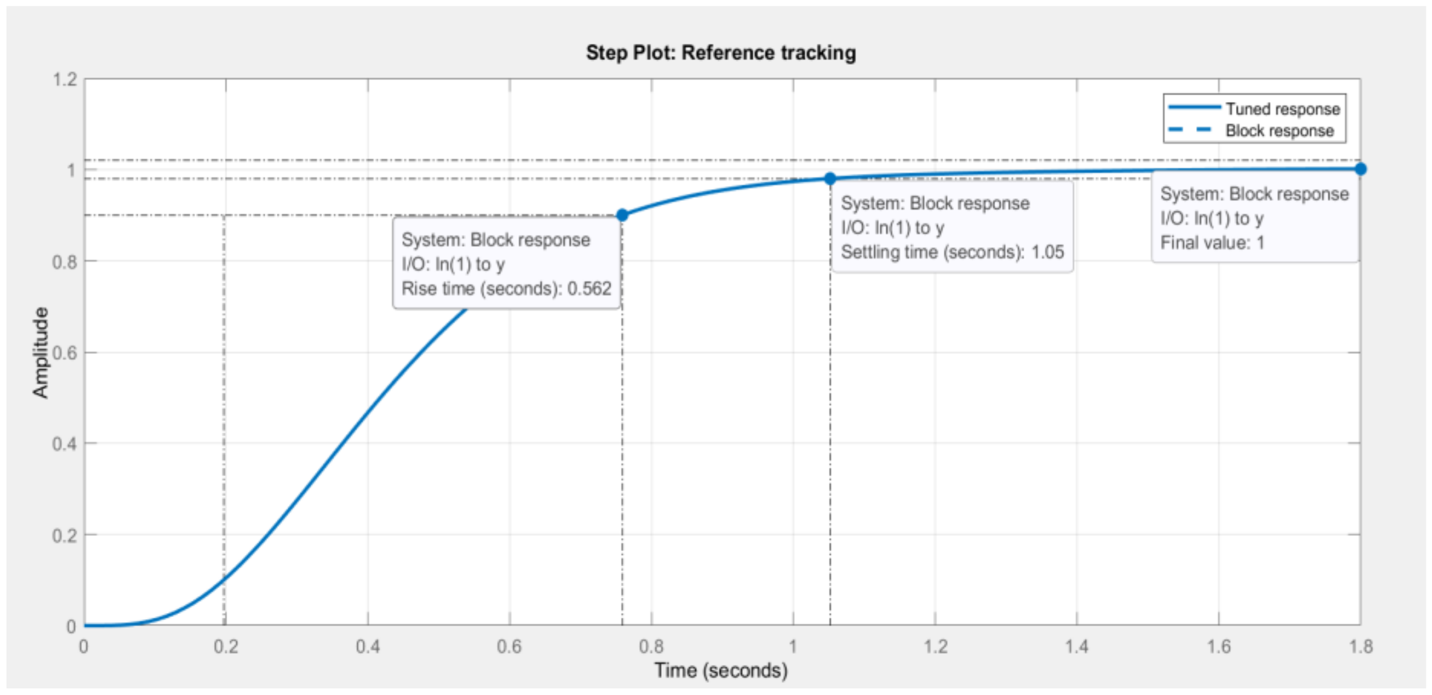
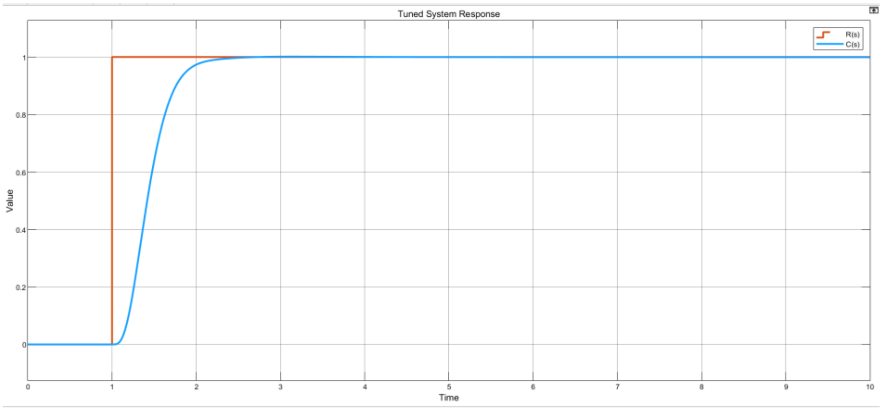
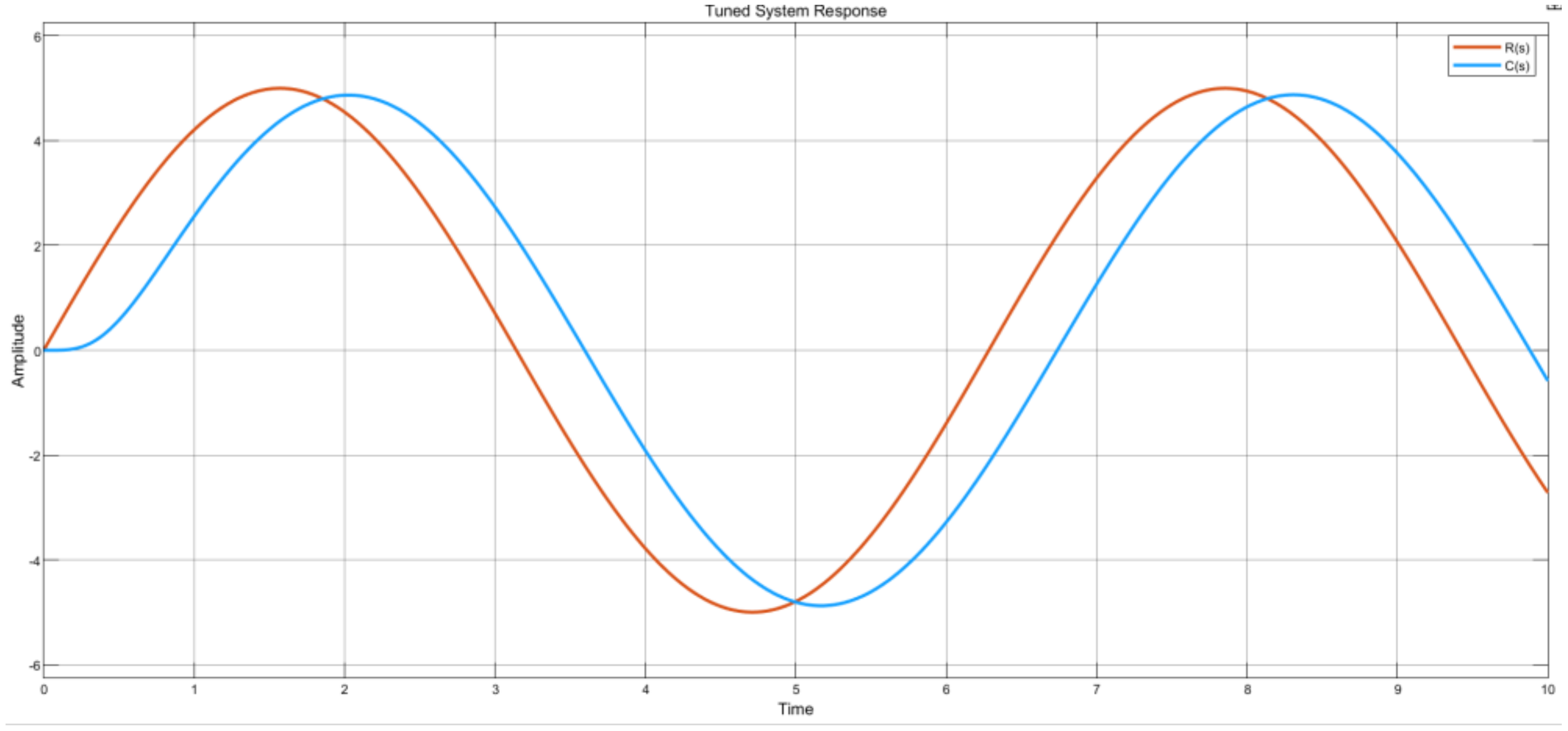
Figure 21.
Fine-tuned system response.
Figure 21.
Fine-tuned system response.
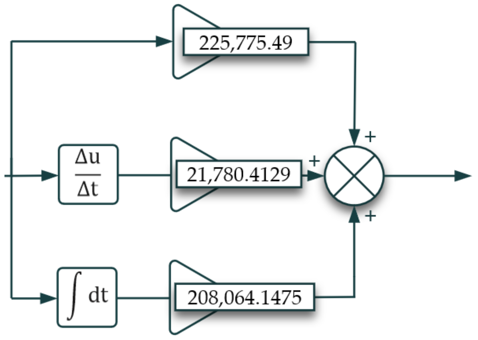
Figure 22.
Tuned PID block expanded view.
Figure 22.
Tuned PID block expanded view.
Figure 23.
Step input source test graph plot.
Figure 23.
Step input source test graph plot.
Figure 24.
Sine wave source graph plot.
Figure 24.
Sine wave source graph plot.
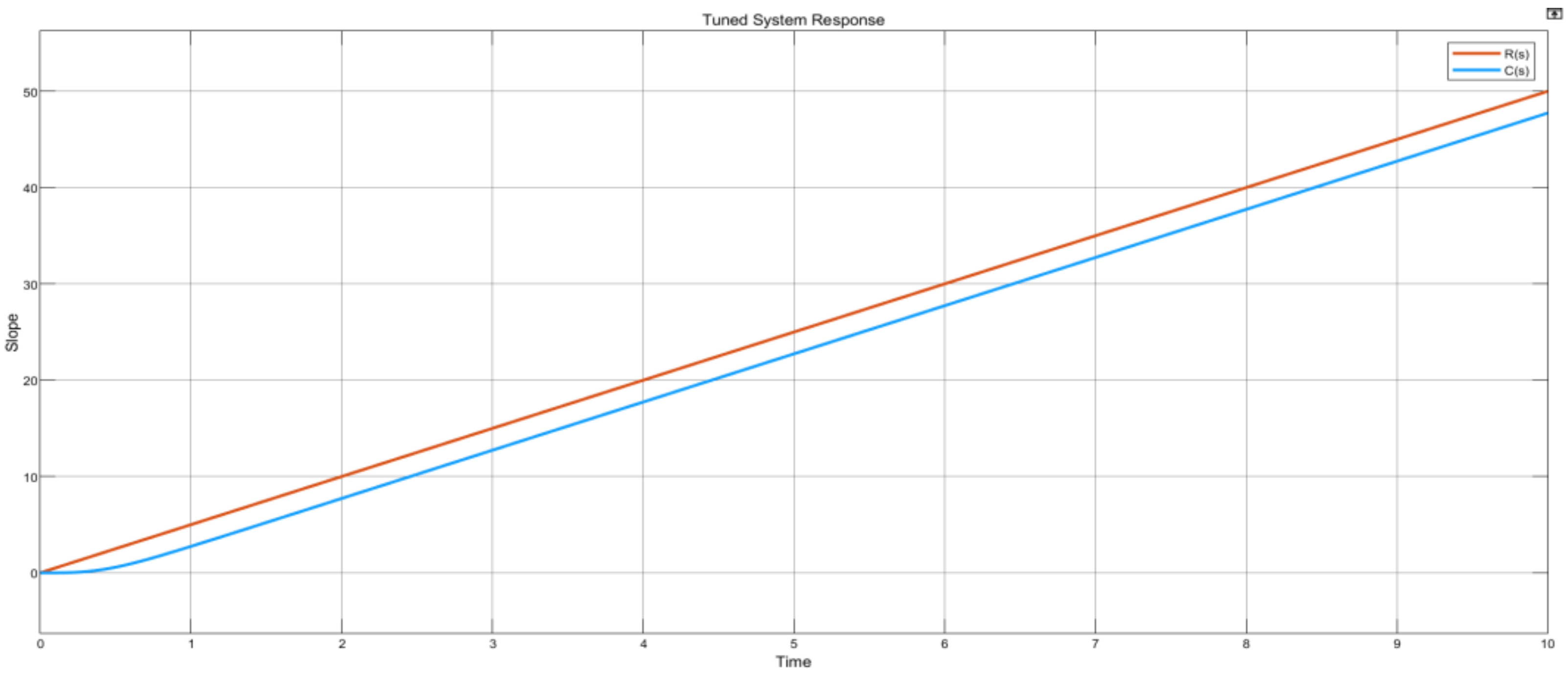
Figure 25.
Ramp source graph plot.
Figure 25.
Ramp source graph plot.
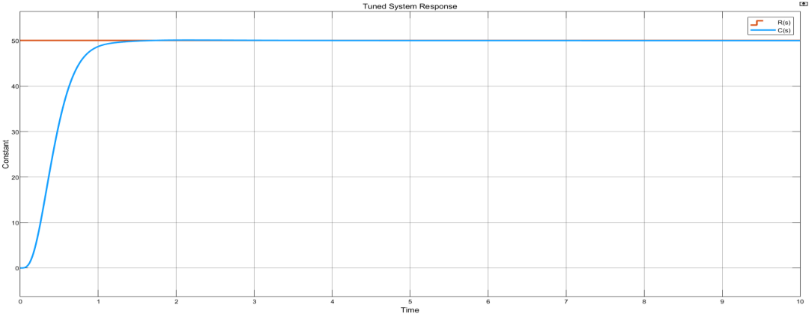
Figure 26.
Constant source graph plot.
Figure 26.
Constant source graph plot.
Figure 27.
Input pressure simulation—0 kPa.
Figure 27.
Input pressure simulation—0 kPa.
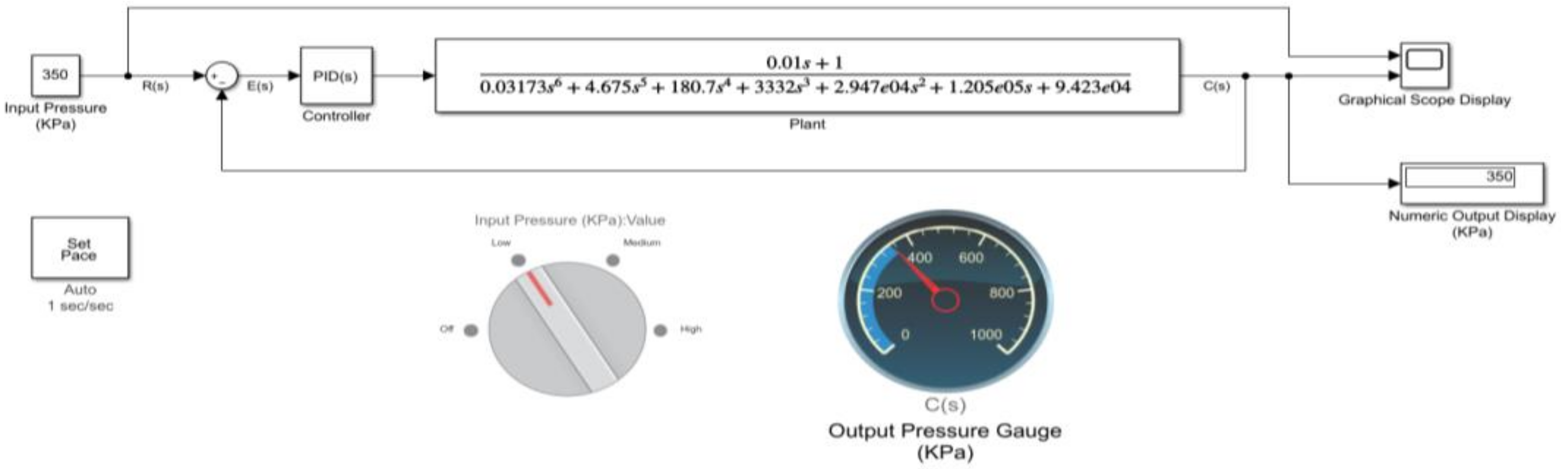
Figure 28.
Input pressure simulation—350 kPa.
Figure 28.
Input pressure simulation—350 kPa.
Figure 29.
Input pressure simulation—750 kPa.
Figure 29.
Input pressure simulation—750 kPa.
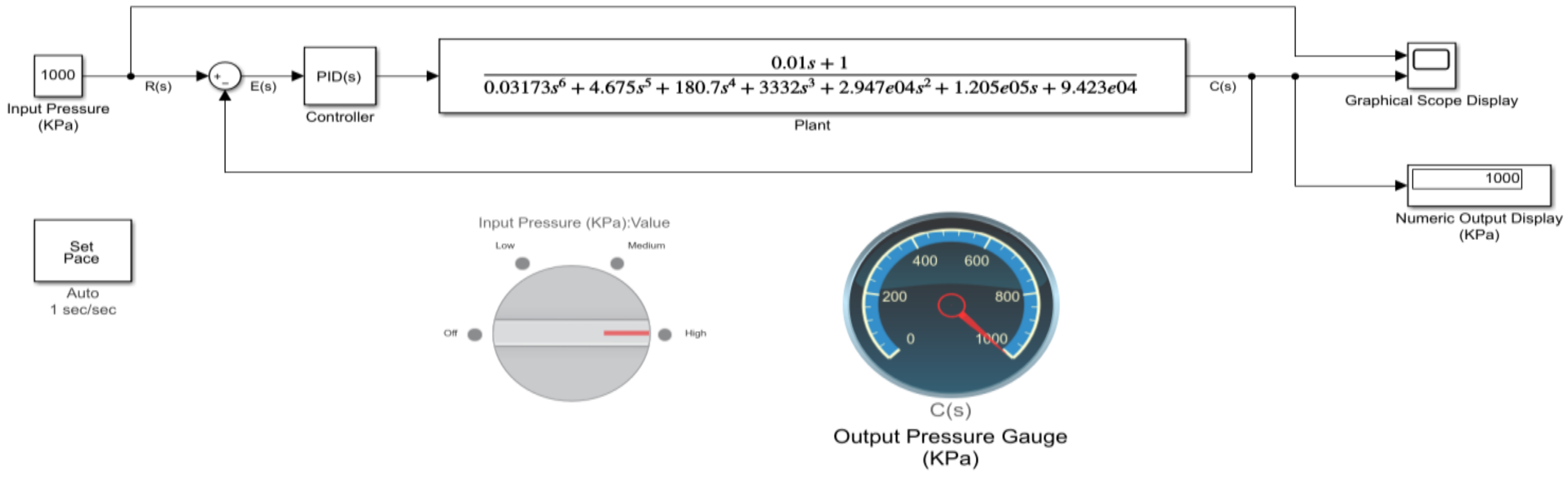
Figure 30.
Input pressure simulation—1000 kPa.
Figure 30.
Input pressure simulation—1000 kPa.
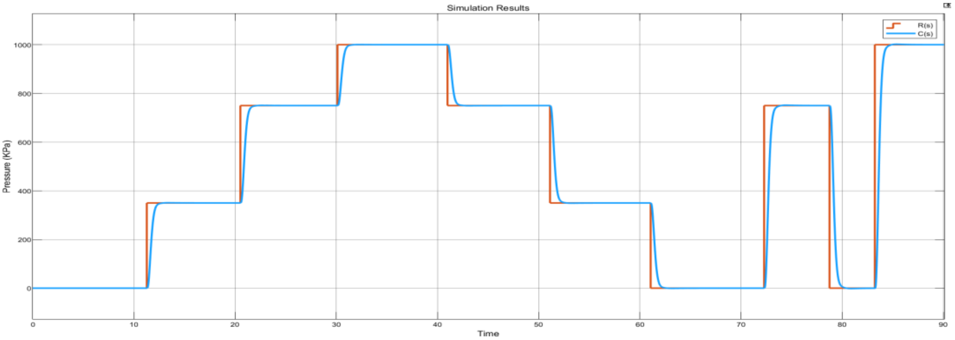
Figure 31.
Varied set points continuous simulation results plot.
Figure 31.
Varied set points continuous simulation results plot.
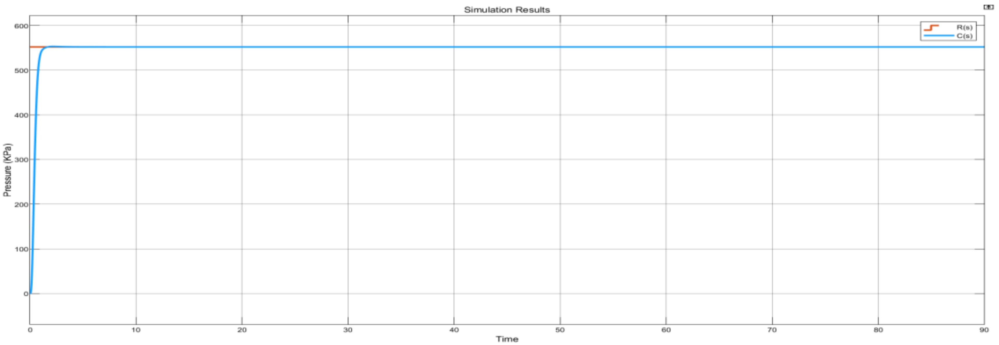
Figure 32.
Input pressure simulation—552 kPa.
Figure 32.
Input pressure simulation—552 kPa.
Figure 33.
Constant set point simulation results plot.
Figure 33.
Constant set point simulation results plot.
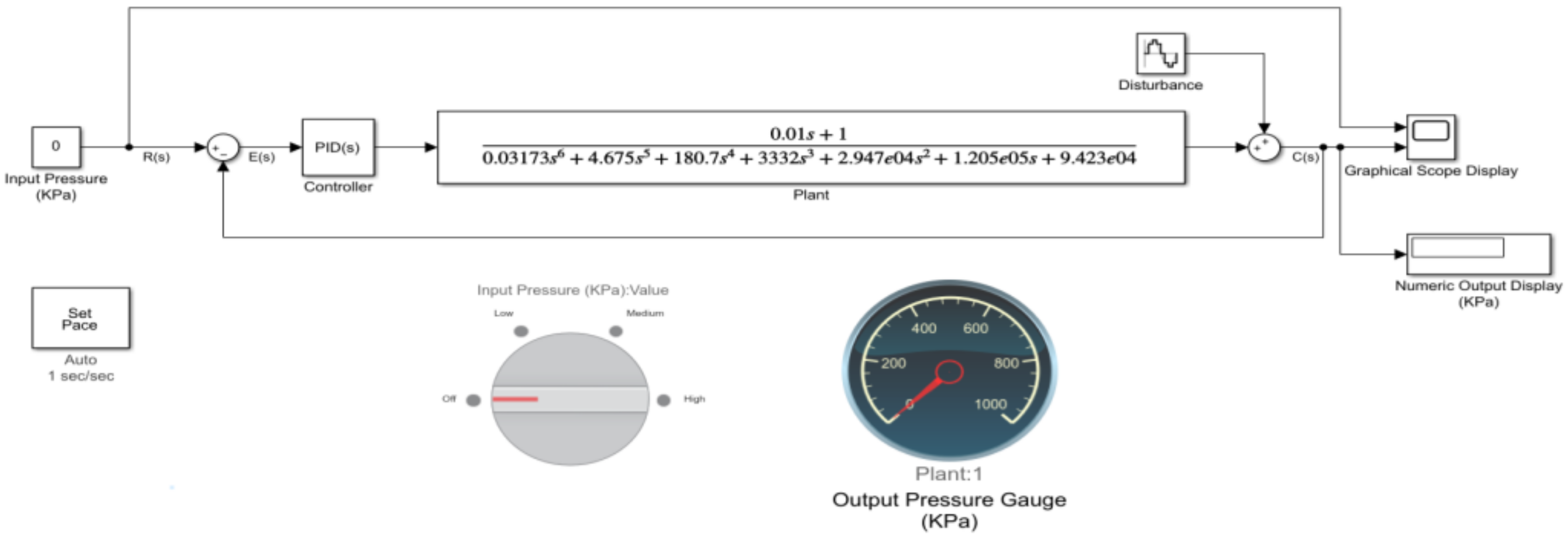
Figure 34.
Disturbance correction configured system.
Figure 34.
Disturbance correction configured system.
Figure 35.
Normal disturbance plot.
Figure 35.
Normal disturbance plot.
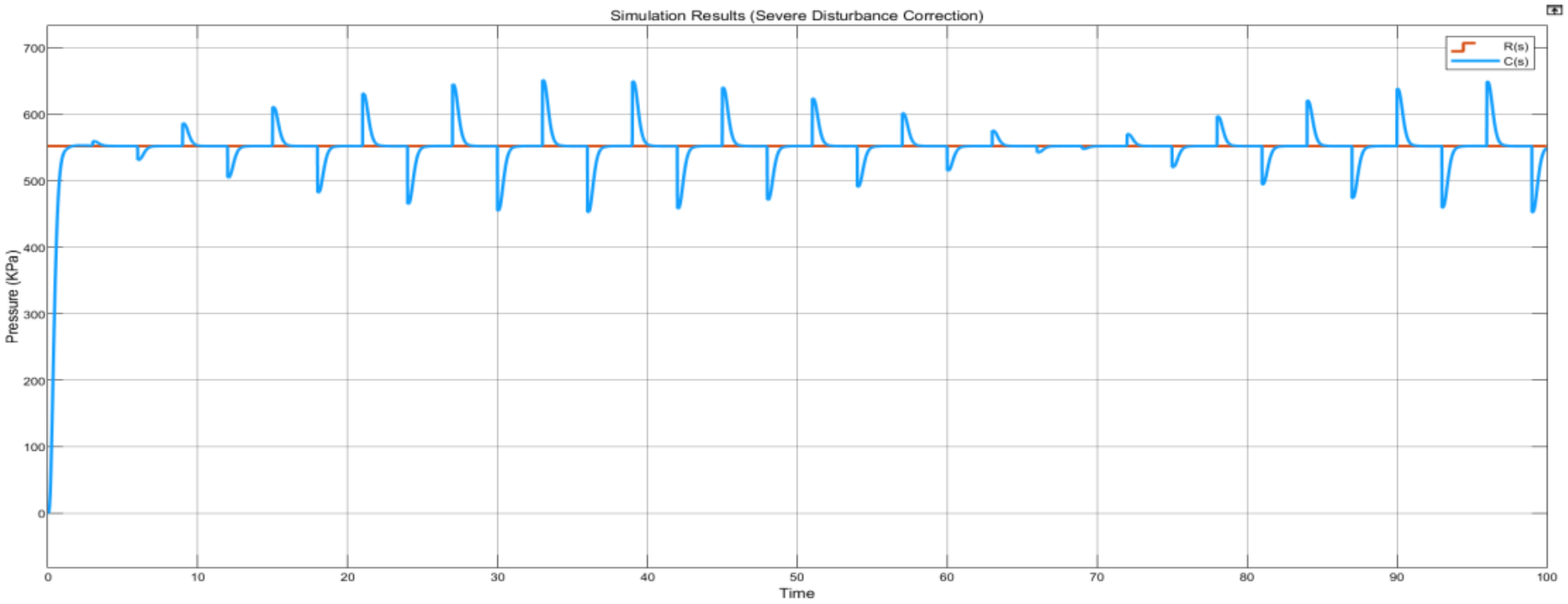
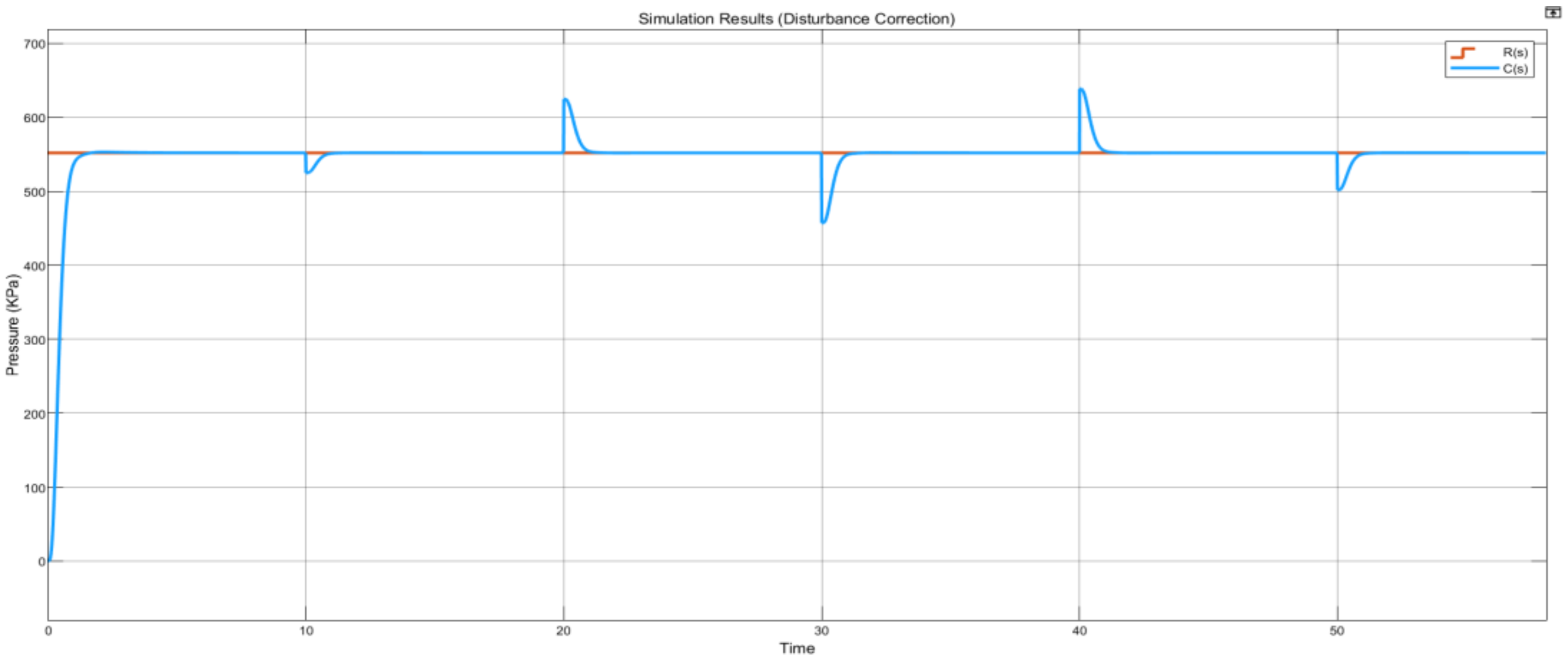
Figure 36.
Severe disturbance plot.
Figure 36.
Severe disturbance plot.
Table 1.
Second DOF mass spring damper variables properties.
Table 1.
Second DOF mass spring damper variables properties.
| Variables | Parameter |
|---|
| m1 | Valve diaphragm mass |
| m2 | Acoustic horn diaphragm mass |
| k1 | Valve spring constant |
| k2 | Force multiplier |
| k3 | Acoustic horn spring constant |
| c1 | Damping coefficient @m1 |
| c3 | Damping coefficient @m2 |
Table 2.
Silicon nitride diaphragm input parameters [
11].
Table 2.
Silicon nitride diaphragm input parameters [
11].
| Parameter | Value |
|---|
| Material | Silicon Nitride |
| Thickness (mm) | 30 |
| Diameter (mm) | 297 |
| Requested accuracy level | Very high |
Table 3.
Physical properties of a silicon nitride diaphragm.
Table 3.
Physical properties of a silicon nitride diaphragm.
| General Properties | Value |
|---|
| Material | Silicon Nitride |
| Density | 3.180 g/cm3 |
| Mass | 6.609 kg (Relative Error = 0.000000%) |
| Area | 166,549.964 mm2 (Relative Error = 0.000000%) |
| Volume | 2,078,375.598 mm3 (Relative Error = 0.000000%) |
Table 4.
Titanium diaphragm input parameters [
12].
Table 4.
Titanium diaphragm input parameters [
12].
| Parameter | Value |
|---|
| Material | Titanium |
| Thickness (mm) | 1 |
| Diameter (mm) | 367 |
| Requested accuracy level | Very high |
Table 5.
Physical properties of a titanium diaphragm.
Table 5.
Physical properties of a titanium diaphragm.
| General Properties | Value |
|---|
| Material | Titanium |
| Density | 4.510 g/cm3 |
| Mass | 0.477 kg (Relative Error = 0.000000%) |
| Area | 212,721.951 mm2 (Relative Error = 0.000000%) |
| Volume | 105,784.493 mm3 (Relative Error = 0.000000%) |
Table 6.
Acoustic horn spring constant input parameters.
Table 6.
Acoustic horn spring constant input parameters.
| Design Inputs |
|---|
| Installed length type | Custom |
| Coil length (mm) | 40 |
| Coil direction | Right Direction |
| Spring start | Closed end coils (µL) | 1.5 |
| Transition coils (µL) | 1 |
| Ground coils (µL) | 0.75 |
| Spring end | Closed end coils (µL) | 1 |
| Transition coils (µL) | 0.75 |
| Ground coils (µL) | 0.5 |
| Calculation Inputs |
| Minimum load length (mm) | 45 |
| Maximum load length (mm) | 39.270 |
| Working stroke (mm) | 5.730 |
| Spring material predetermined values | Ultimate tensile stress (MPa) | 1860 |
| Allowable torsional stress (MPa) | 930 |
| Modulus of elasticity in shear (MPa) | 68,500 |
| Density (kg/m3) | 7850 |
| Utilization factor of material (µL) | 0.9 |
Table 7.
Acoustic horn’s spring properties.
Table 7.
Acoustic horn’s spring properties.
| General Properties | Value |
|---|
| ) | 3.172 mm |
| ) | 3802 mm |
| ) | 1 µL |
| ) | 0.175 N/mm |
| ) | 29,649 mm |
| ) | 34,379 mm |
| ) | 60,262 mm |
| ) | 16,872 mm |
| ) | 13,388 mm |
| ) | 10,517 N |
| ) | 377,287 MPa |
| ) | 452,744 MPa |
| ) | 793,600 MPa |
| ) | 10,394 mps |
| ) | 200,787 Hz |
| ) | 0.103 J |
| ) | 509,767 mm |
| ) | 0.001 kg |
Table 8.
Multiple subsystem parameters summary.
Table 8.
Multiple subsystem parameters summary.
| Electrical Systems |
|---|
| 1 Ω |
| 1 F |
| 0.01 Ω |
| 1 Ns/m |
| Mechanical Systems |
| 6.61 kg |
| 0.48 kg |
| 538.47 N/m |
| 1 N/m |
| 175 N/m |
| 98.55 Ns/m |
| 15.09 Ns/m |
Table 9.
Controller design requirements.
Table 9.
Controller design requirements.
| Parameter | Value |
|---|
| ) | 0.5 s |
| ) | 1.5 s |
| % Overshoot | 0–0.9% |
| Closed-loop stability | Stable |
| Aggressive/Robust | Robust |
Table 10.
Control system operating requirements.
Table 10.
Control system operating requirements.
| Parameter | Value |
|---|
| ) | 0.5 s |
| ) | 1.5 s |
| % Overshoot | 0–0.9 |
| Closed-loop stability | Stable |
Table 11.
PID tuning settings.
Table 11.
PID tuning settings.
| Parameter | Value |
|---|
| Controller | PID |
| Time domain | Continuous-time |
| Form | Parallel |
| Source | Internal |
| Tuning method | Transfer function based |
| Zero-crossing detection | Enabled |
| Compensator formula | |
Table 12.
Tuned controller parameters.
Table 12.
Tuned controller parameters.
| Parameter | Tuned | Block |
|---|
| P | 183,706.2513 | 1 |
| I | 232,966.3411 | 1 |
| D | 30,144.1142 | 1 |
| N | 206.9837 | 100 |
Table 13.
Tuned system performance and robustness.
Table 13.
Tuned system performance and robustness.
| Parameter | Tuned | Block |
|---|
| Rise time | 0.752 s | 2.07 × 10⁵ s |
| Settling time | 3.13 s | 3.69 × 10⁵ s |
| Overshoot | 5.98% | 0% |
| Peak | 1.06 | 1 |
| Gain margin | 15.7 dB @ 10.3 rad/s | 109 dB @ 12.4 rad/s |
| Phase margin | 69 deg @ 1.81 rad/s | 90 deg @ 1.06 × 10⁻⁵ rad/s |
| Compensator formula | Stable | Stable |
Table 14.
Fine-tuned controller parameters.
Table 14.
Fine-tuned controller parameters.
| Parameter | Tuned | Block |
|---|
| P | 225,775.49 | 225,775.49 |
| I | 208,064.1457 | 208,064.1457 |
| D | 21,780.4129 | 21,780.4129 |
| N | 248.1711 | 248.1711 |
Table 15.
Fine-tuned system performance and robustness.
Table 15.
Fine-tuned system performance and robustness.
| Parameter | Tuned | Block |
|---|
| Rise time | 0.562 s | 0.562 s |
| Settling time | 1.05 s | 1.05 s |
| Overshoot | 0.201% | 0.201% |
| Peak | 1 | 1 |
| Gain margin | 14.2 dB @ 8.81 rad/s | 14.2 dB @ 8.81 rad/s |
| Phase margin | 69 deg @ 2.17 rad/s | 69 deg @ 2.17 rad/s |
| Compensator formula | Stable | Stable |
Table 16.
Design summary of results.
Table 16.
Design summary of results.
| Parameter | Requirement | Actual Controller Design | Actual Control System Design |
|---|
| ) | 0.6 s | 0.562 s | 0.562 s |
| ) | 1.5 s | 1.05 s | 1.05 s |
| % Overshoot | 0–0.9% | 0.201% | 0.201% |
| Closed-loop stability | Stable | Stable | Stable |
| Aggressive/Robust | Robust (0.69) | Robust (0.6) | Robust (0.6) |
Table 17.
Input pressure scenarios.
Table 17.
Input pressure scenarios.
| Set-Point | Pressure |
|---|
| Off | 0 kPa |
| Low | 350 kPa |
| Mid | 750 kPa |
| High | 1000 kPa |
Table 18.
Acoustic system components [
24].
Table 18.
Acoustic system components [
24].
| Component | Recommendation |
|---|
| Solenoid valves | 1 per horn, 1 per system |
| Manual isolation valve | 1 per horn, 1 per system |
| Flow regulator | Air type based regulator |
| Flex | Stainless steel material |
Table 19.
Research novelty subsystem comparison.
Table 19.
Research novelty subsystem comparison.
| Industry Standard Configuration | Research System Components |
|---|
| Solid-state electronic timer | I-P transducer |
| Solenoid valve | Spring and diaphragm valve |
| No feedback transducer | Piezoresistive pressure sensor |
| Industry Standard Configuration | Research System Components |


