Simulations and Subjective Rating of Acoustic Conditions in a Symphony Orchestra—A Case Study


Abstract
:1. Introduction
1.1. Literature Review and Previous Research in Stage Acoustics
1.2. Case Background
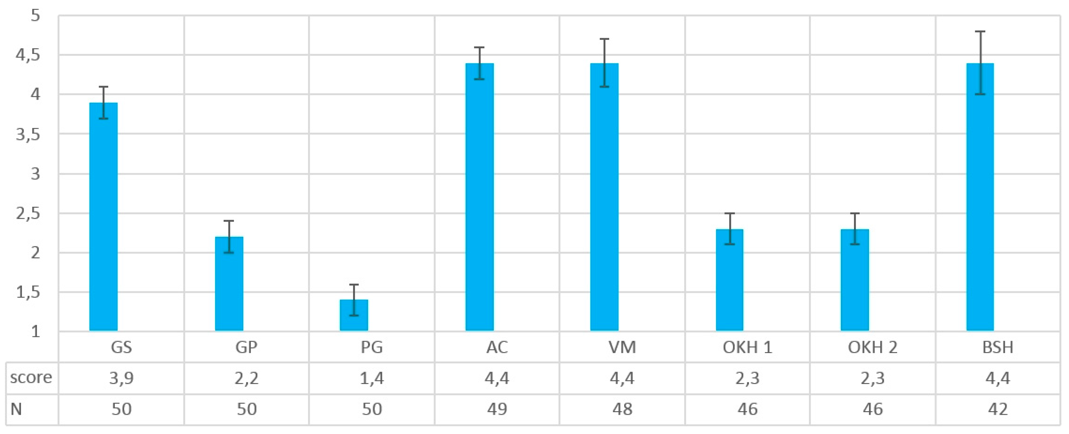
1.3. Subjective Data
1.4. Objective Data—Compact Definitions of Metrics (Parameters)
| G | (dB) | Sound Strength, in decibels, sound pressure level at arbitrary distance from omni-directional source, relative to level of direct sound at 10-m distance from the same source |
| Gd | (dB) | G from the direct sound component only, i.e., G in anechoic condition |
| Gr | (dB) | Strength of reflected, i.e., reverberant, sound |
| Glate | (dB) | Strength of reflected sound arriving 80 ms or later after direct sound |
| T30 | (s) | Reverberation time of a room, calculated from the slope of the decaying sound tail, in the 30-dB interval between −5 and −35 dB |
| STearly | (dB) | Stage support, level of reflected sound energy in the 20–100 ms interval, related to energy in the 10–20 ms interval, from an omni-directional source at 1-m distance, average of octave bands 250 through 1000 Hz |
| STlate | (dB) | Stage support, level of reflected sound energy in the 100–1000 ms interval, related to energy in the 10–20 ms interval, from an omni-directional source at 1-m distance, average of octave bands 250 through 1000 Hz |
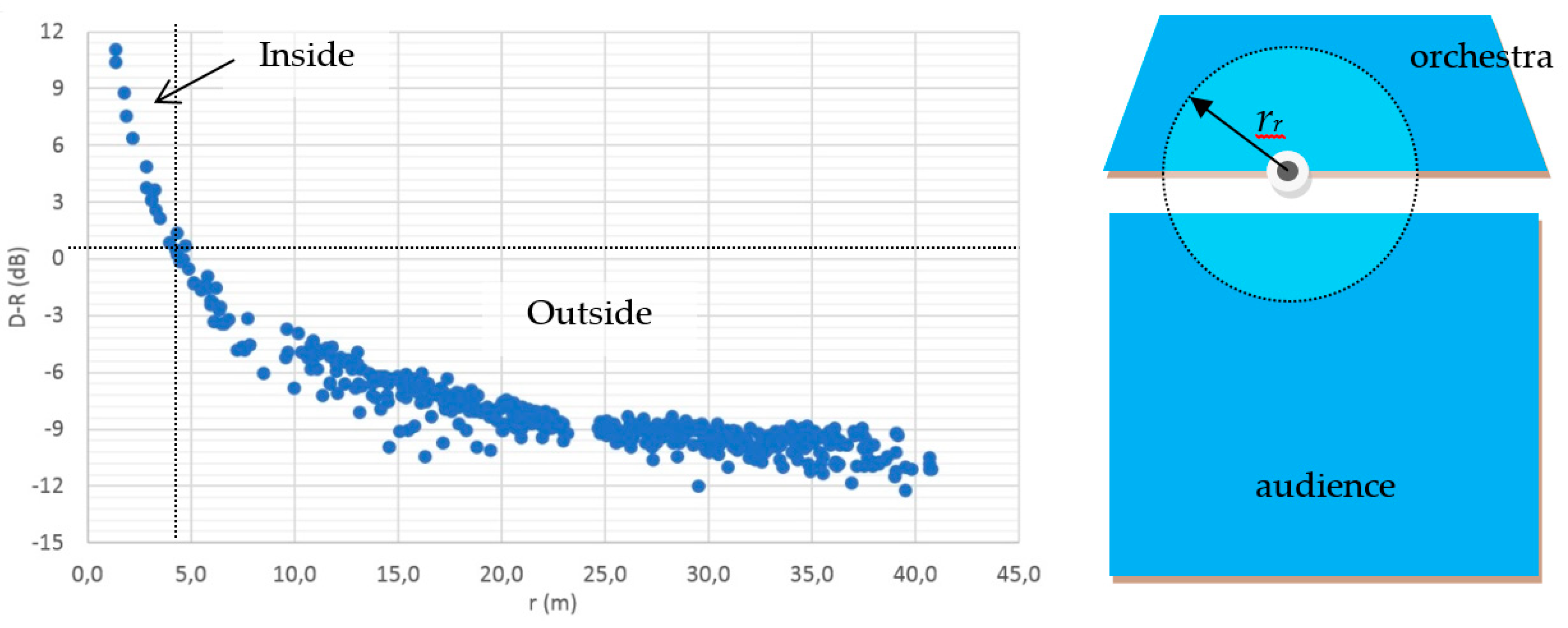
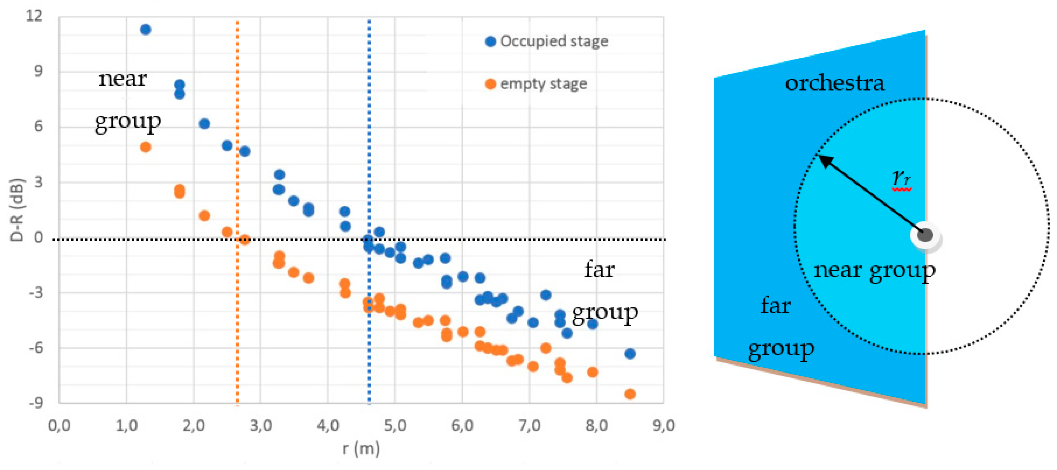
| D-R | (dB) | Direct-to-reverberant sound level balance, D-R = Gd-Gr, i.e., 10 × lg(d/r) where d/r is the ratio between direct and reverberant sound energy |
2. Method
2.1. 3-D Models for Simulation
2.2. Source, Receivers, and Parameters in the Simulations
3. Result
3.1. Predicted Data—Simulated Room Acoustical Parameters
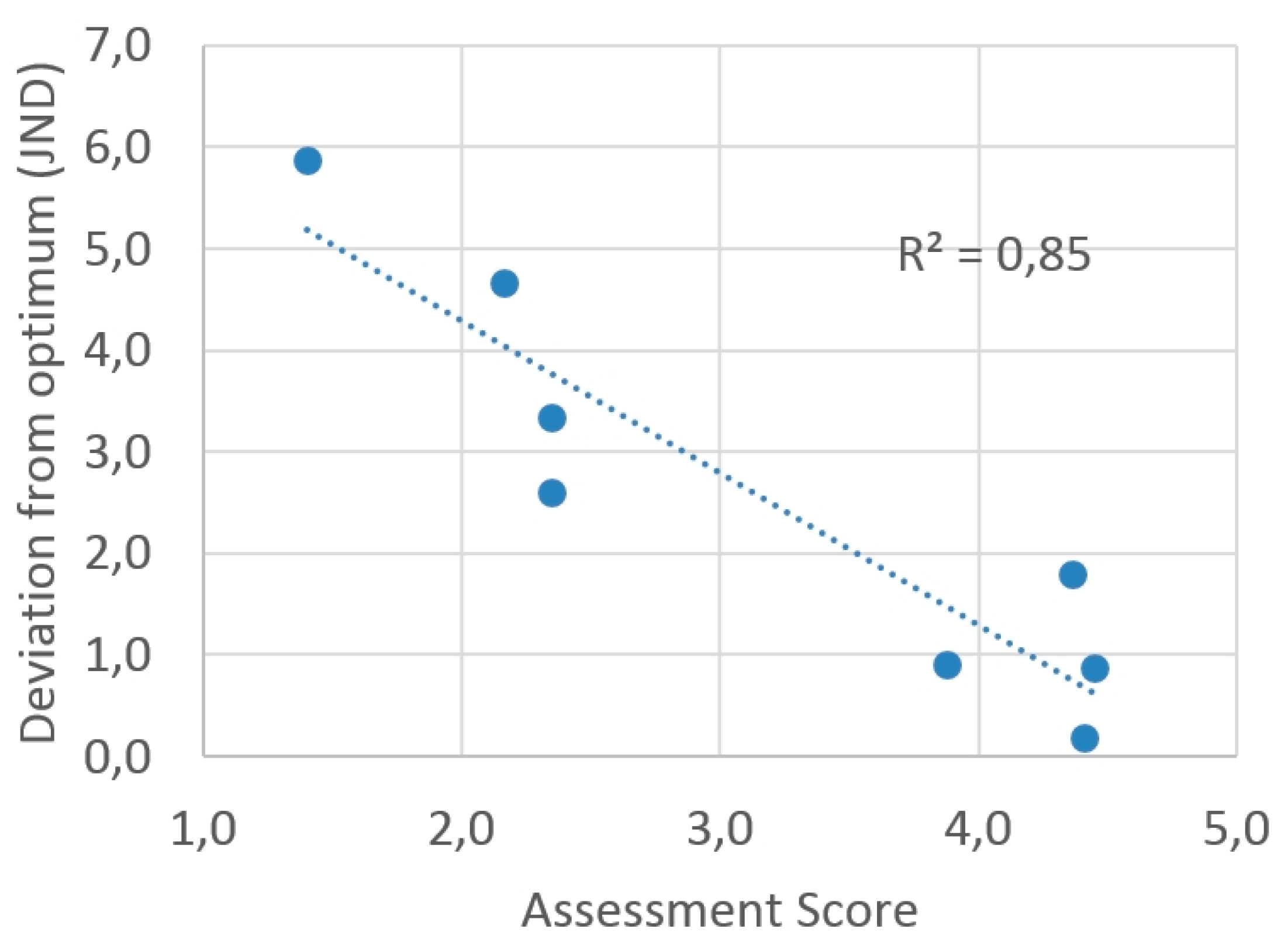
3.2. Correlation Between Subjective and Predicted Data
3.3. First Sight Comments to Correlation Results
4. Discussion
4.1. Direct-to-Reverberant Ratio and Balance
4.2. Interpretation of BPO’s Preference
5. Outlooking
5.1. Two Sides of the Same Coin
5.2. Understanding Self-Reinforcing Effects and the Escalating Levels Problem
5.3. Further Work
6. Conclusions
Supplementary Materials
Conflicts of Interest
References
- Gade, A.C. Acoustics for Symphony Orchestras; Status After Three Decades of Experimental Research. In Proceedings of the International Symposium on Room Acoustics (ISRA 2010), Melbourne, Australia, 29–31 August 2010; Available online: http://www.akutek.info/Papers/AG_Stage_Acoustics.pdf (accessed on 31 August 2010).
- International Standard. ISO-3382 Acoustics—Measurement of Room Acoustic Parameters—Part 1, Performance Spaces, 1st ed.; International Organization for Standardization, Chemin de Blandonnet 8, CP 401 - 1214 Vernier: Geneva, Switzerland, 2009. [Google Scholar]
- Krokstad, A.; Vindspoll, J.; Sæther, R. Orkesterpodium, Samspill og Solo (Orchestra Platform, Ensemble and Solo); Technical Report; The Laboratory of Acoustics, The Technical University of Trondheim: Trondheim, Norway, 1980. [Google Scholar]
- Halmrast, T. Acoustical Society of America, Chicago 4th June 2001, Session: “The First 80 Milliseconds in Auditoria”. Available online: http://www.akutek.info/Papers/TH_Coloration2001.pdf (accessed on 13 March 2007).
- Skålevik, M. Sound Transmission between Musicians in a Symphony Orchestra on a Concert Hall Stage. 2007. Available online: http://www.akutek.info/Papers/MS_Sound_Transmission.pdf (accessed on 17 May 2007).
- Dammerud, J.J. Stage Acoustics for Symphony Orchestras in Concert Halls. Chapter 4. Available online: http://www.akutek.info/Papers/JJD_Stage_acoustics_PhDthesis_96dpi.pdf (accessed on 20 May 2010).
- Wenmaekers, R.H.C.; Hak, C.C.J.M. Noise Exposure of Musicians: The Own Instrument’s Sound Compared to the Sound from Others (Euronoise, Maastricht 2015). Available online: http://www.akutek.info/Papers/RW_Own_Instrument_reOthers.pdf (accessed on 8 June 2015).
- Skålevik, M. Level Balance between Self, Others and Reverb, and Its Significance to Noise Exposure as Well as Mutual Hearing in Orchestra Musicians, (Euronoise, Maastricht 2015). Available online: http://www.akutek.info/Papers/MS_Self_Others_Reverb.pdf (accessed on 5 June 2015).
- Gade, A.C. Sound levels in rehearsal and medium sized concert halls; are they too loud for the musicians? In Proceedings of the Meetings on Acoustics, Hong Kong, China, 13–18 May 2012. [Google Scholar]
- Directivity of Musical Instruments. Available online: http://www.akutek.info/articles_files/dynamic_directivity.htm (accessed on 9 December 2011).
- Jeffress, L.A. A place theory of sound localization. J. Comp. Physiol. Psychol. 1948, 41, 35–39. [Google Scholar] [CrossRef]


| Venue | Gr-Gd (dB) | Gr (dB) | T30 (s) | Glate (dB) | STlate (dB) | G (dB) | STearly (dB) | Gd (dB) |
|---|---|---|---|---|---|---|---|---|
| GS | 1 | 8 | 1.7 | 2 | −18 | 11 | −15 | 7 |
| GP | 5 | 10 | 1.0 | −4 | −25 | 12 | −14 | 5 |
| PG | 6 | 13 | 1.4 | 9 | −13 | 14 | −12 | 7 |
| AC | −2 | 5 | 2.1 | 1 | −20 | 9 | −19 | 6 |
| VM | 0 | 7 | 2.0 | 2 | −18 | 10 | −12 | 7 |
| OKH 1 | −3 | 4 | 1.5 | 0 | −21 | 9 | −16 | 7 |
| OKH 2 | −3 | 3 | 1.6 | 0 | −21 | 9 | −18 | 7 |
| BS | −1 | 5 | 2.2 | 0 | −22 | 9 | −19 | 6 |
| X | 0 | 7 | 2.2 | 2 | −19 | 10 | −20 | 6 |
| Venue | Gr-Gd (JND) | Gr (JND) | T30 (JND) | Glate (JND) | STlate (JND) | G (JND) | STearly (JND) | Gd (JND) | Score |
|---|---|---|---|---|---|---|---|---|---|
| GS | 1 | 1 | 4 | 0 | 1 | 1 | 5 | 1 | 3.9 |
| GP | 5 | 3 | 11 | 6 | 6 | 2 | 6 | 1 | 2.2 |
| PG | 6 | 6 | 7 | 7 | 6 | 4 | 8 | 1 | 1.4 |
| AC | 2 | 2 | 1 | 1 | 1 | 1 | 1 | 0 | 4.4 |
| VM | 0 | 0 | 2 | 0 | 1 | 0 | 8 | 1 | 4.4 |
| OKH 1 | 3 | 3 | 6 | 2 | 2 | 1 | 5 | 1 | 2.3 |
| OKH 2 | 3 | 3 | 5 | 2 | 2 | 1 | 2 | 1 | 2.3 |
| BSH | 1 | 1 | 0 | 2 | 3 | 1 | 1 | 0 | 4.4 |
| r2 | 0.85 | 0.74 | 0.71 | 0.64 | 0.51 | 0.49 | 0.22 | 0.09 | 1.0 |
| r | −0.92 | −0.86 | −0.84 | −0.8 | −0.71 | −0.7 | −0.47 | −0.29 | −1.0 |
© 2019 by the author. Licensee MDPI, Basel, Switzerland. This article is an open access article distributed under the terms and conditions of the Creative Commons Attribution (CC BY) license (http://creativecommons.org/licenses/by/4.0/).
Share and Cite
Skålevik, M. Simulations and Subjective Rating of Acoustic Conditions in a Symphony Orchestra—A Case Study. Acoustics 2019, 1, 570-581. https://doi.org/10.3390/acoustics1030033
Skålevik M. Simulations and Subjective Rating of Acoustic Conditions in a Symphony Orchestra—A Case Study. Acoustics. 2019; 1(3):570-581. https://doi.org/10.3390/acoustics1030033
Chicago/Turabian StyleSkålevik, Magne. 2019. "Simulations and Subjective Rating of Acoustic Conditions in a Symphony Orchestra—A Case Study" Acoustics 1, no. 3: 570-581. https://doi.org/10.3390/acoustics1030033
APA StyleSkålevik, M. (2019). Simulations and Subjective Rating of Acoustic Conditions in a Symphony Orchestra—A Case Study. Acoustics, 1(3), 570-581. https://doi.org/10.3390/acoustics1030033