
Localized Corrosion of Mooring Chain Steel in Seawater


Abstract
:1. Introduction
2. Experimental
2.1. Materials
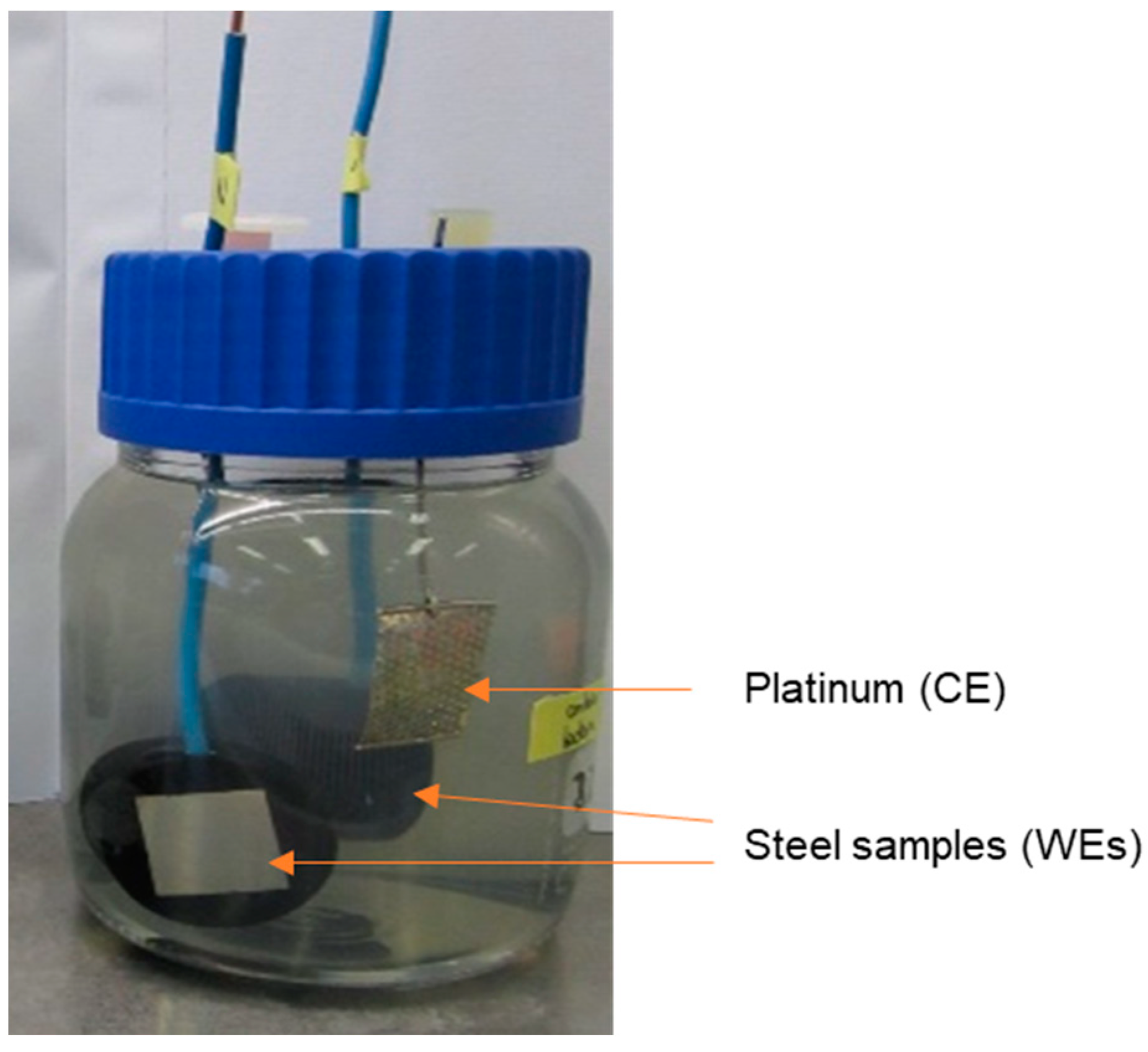
2.2. Experimental Set-Up
2.3. Electrolytes
2.4. Inoculation of Microorganisms
2.5. Electrochemical Measurements
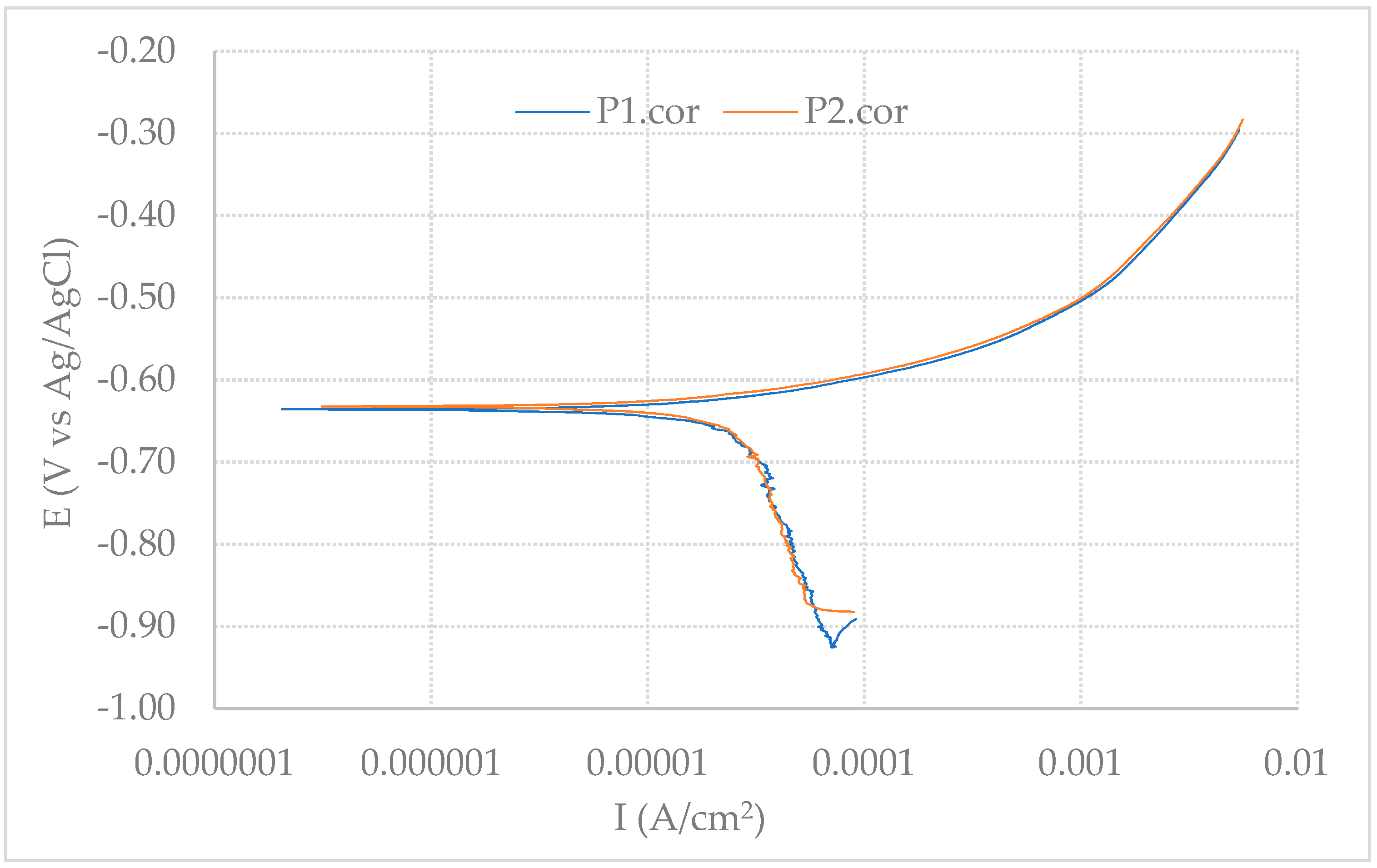
2.5.1. Potentiodynamic Polarization (PDP) Curve Measurements
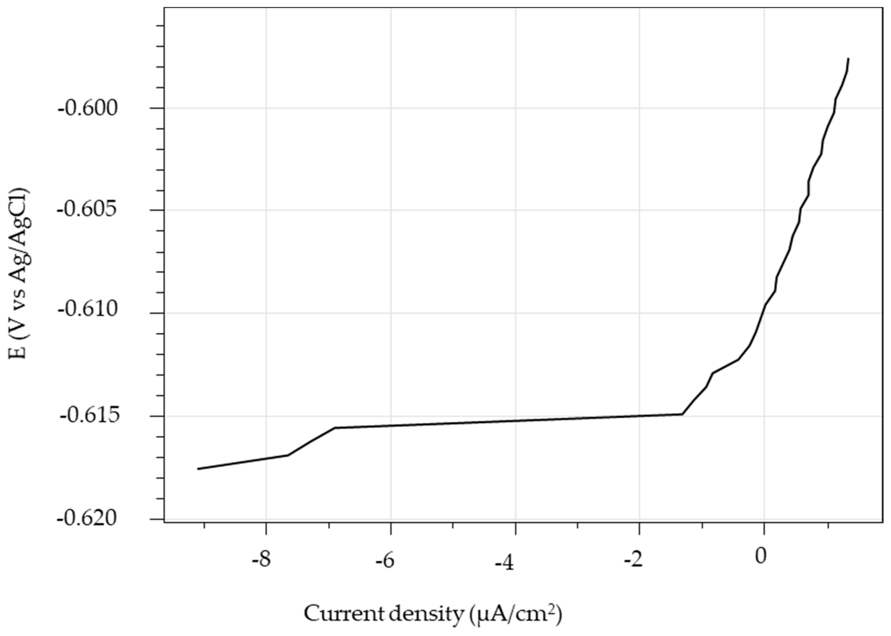
2.5.2. Linear Polarization Resistance (LPR) and Electrochemical Impedance Spectroscopy (EIS) Measurements
2.6. Surface Analysis
2.6.1. Epi-Fluorescence Microscopy
2.6.2. Photo-Microscopy
2.6.3. Scanning Electron Microscopy (SEM)
3. Results
3.1. Electrochemical Measurements
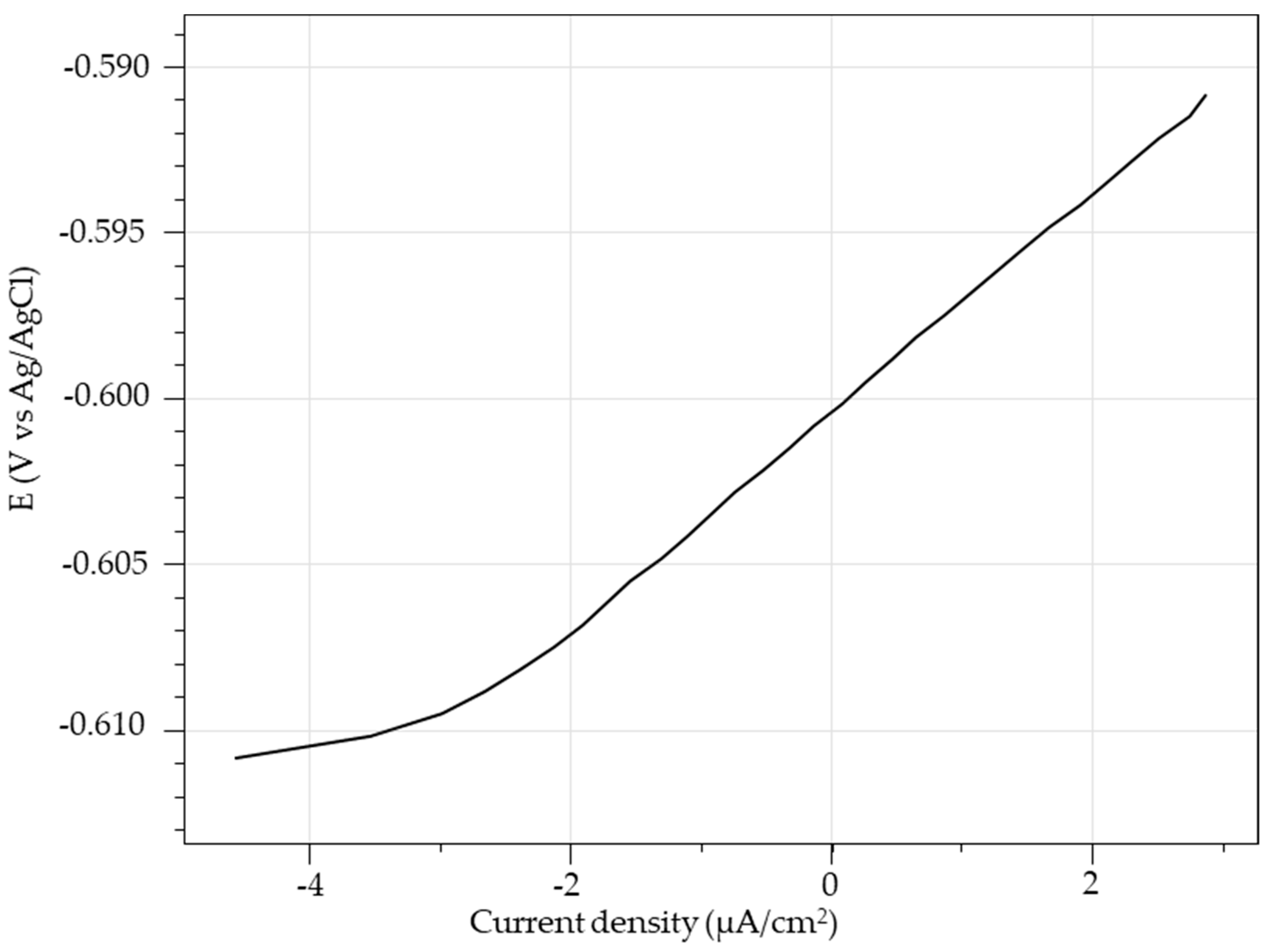
3.1.1. PDP Curve Measurements
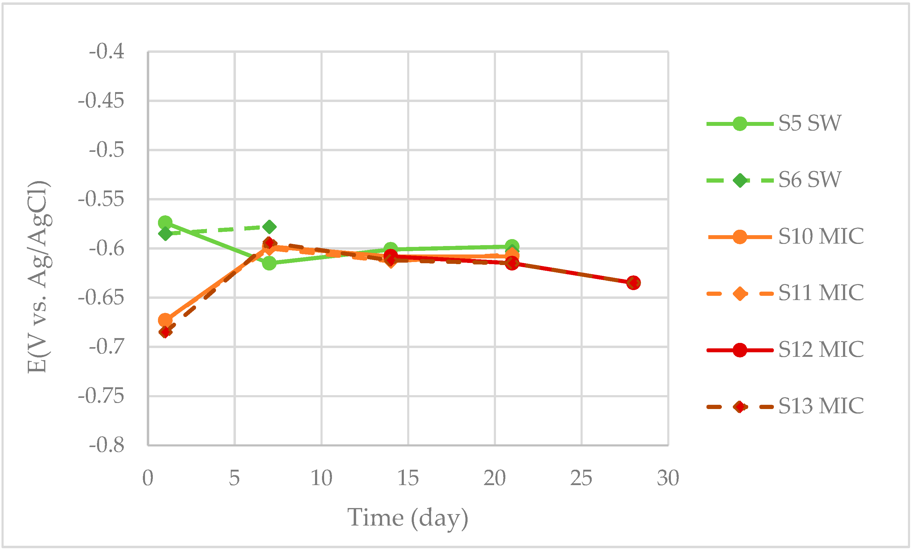
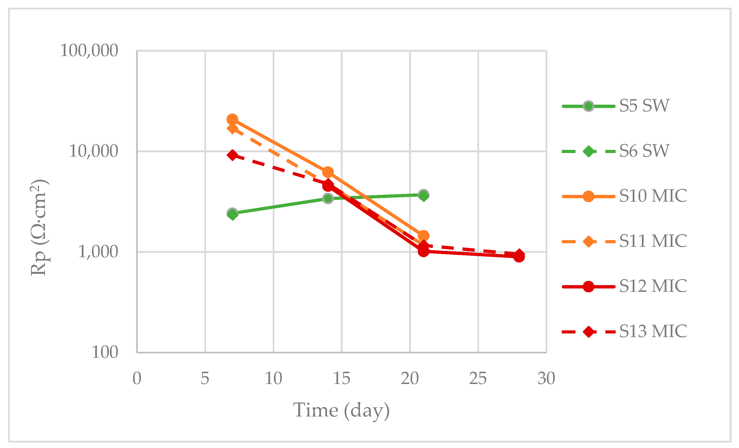
3.1.2. LPR Measurements
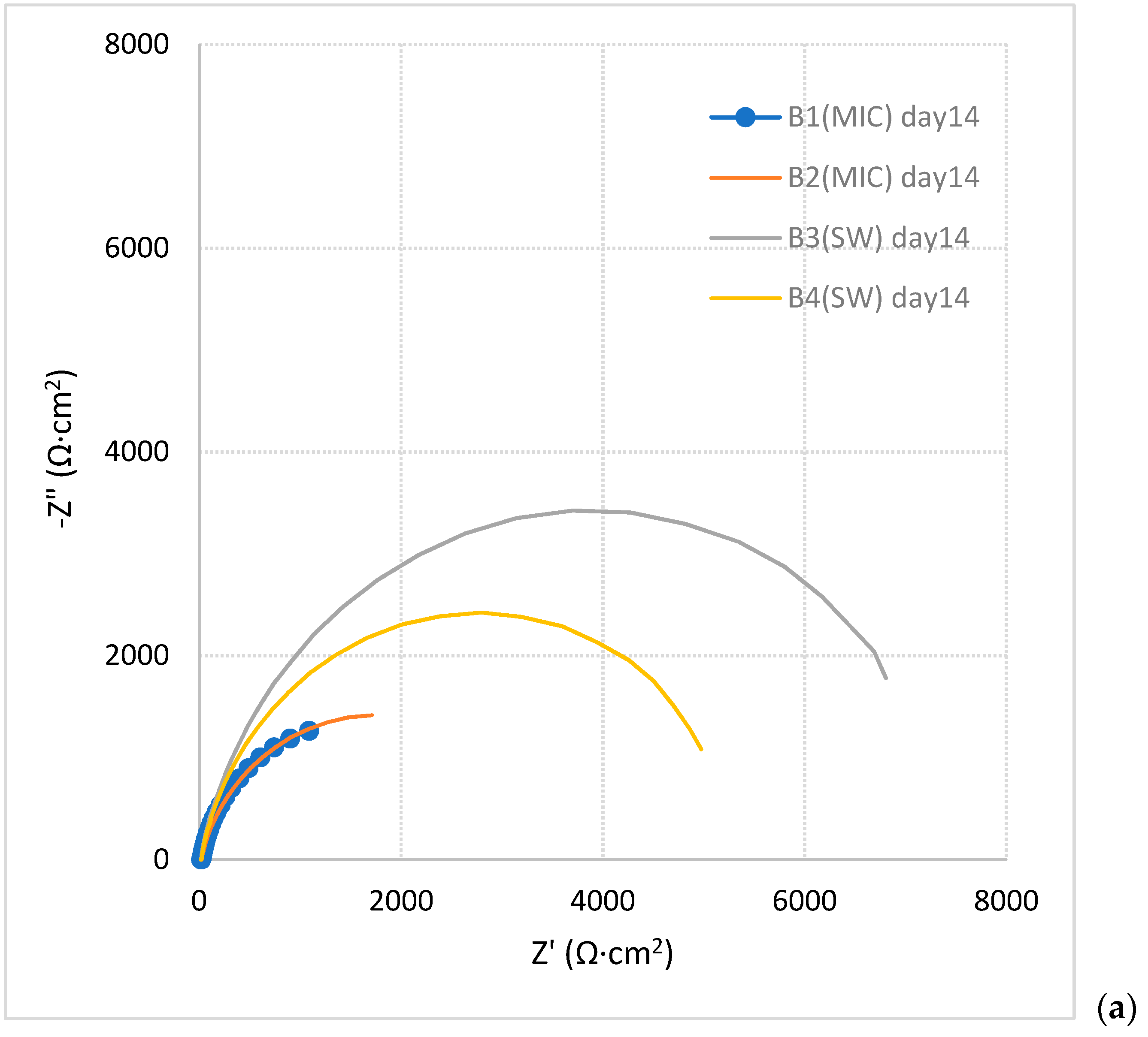
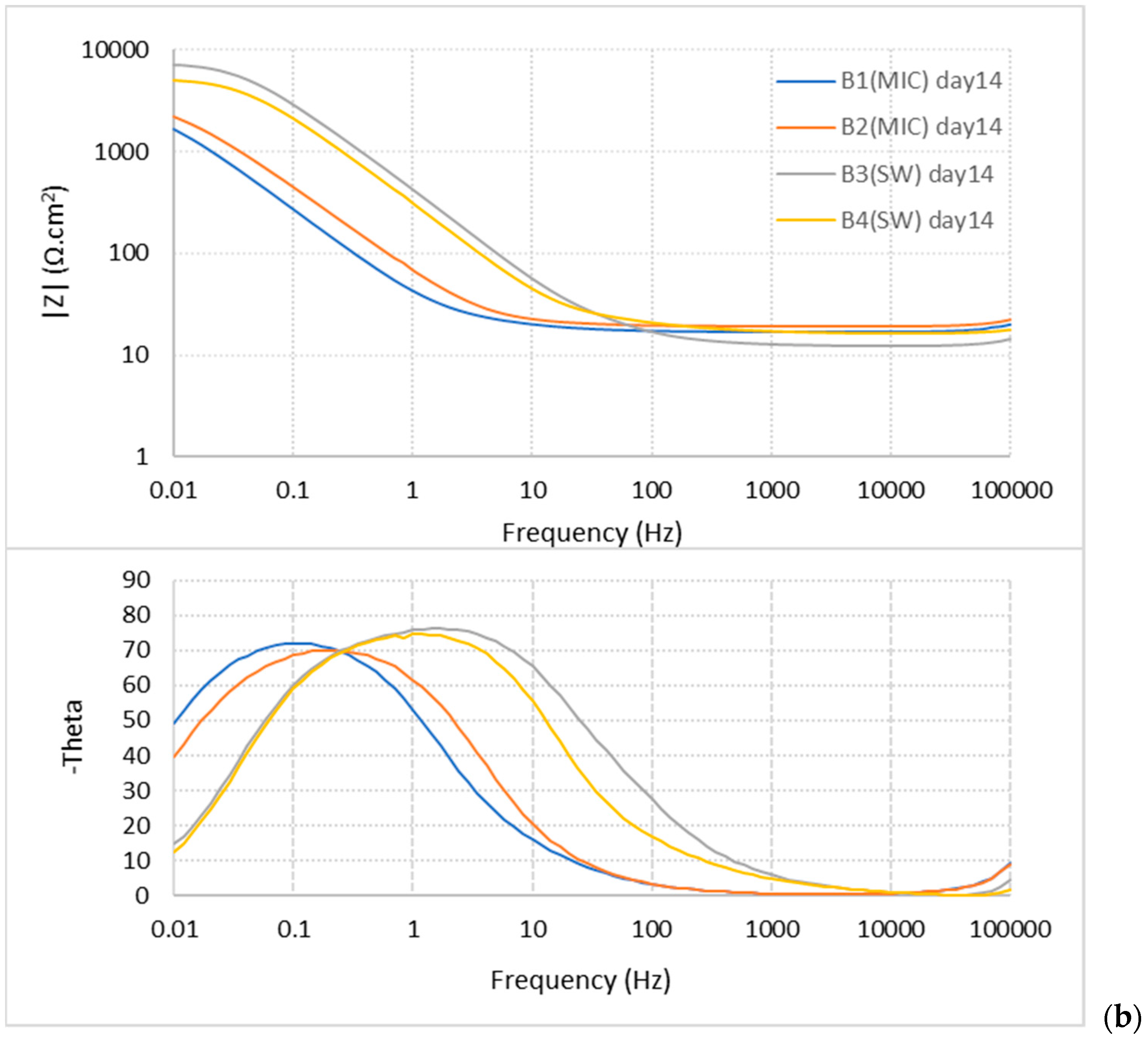
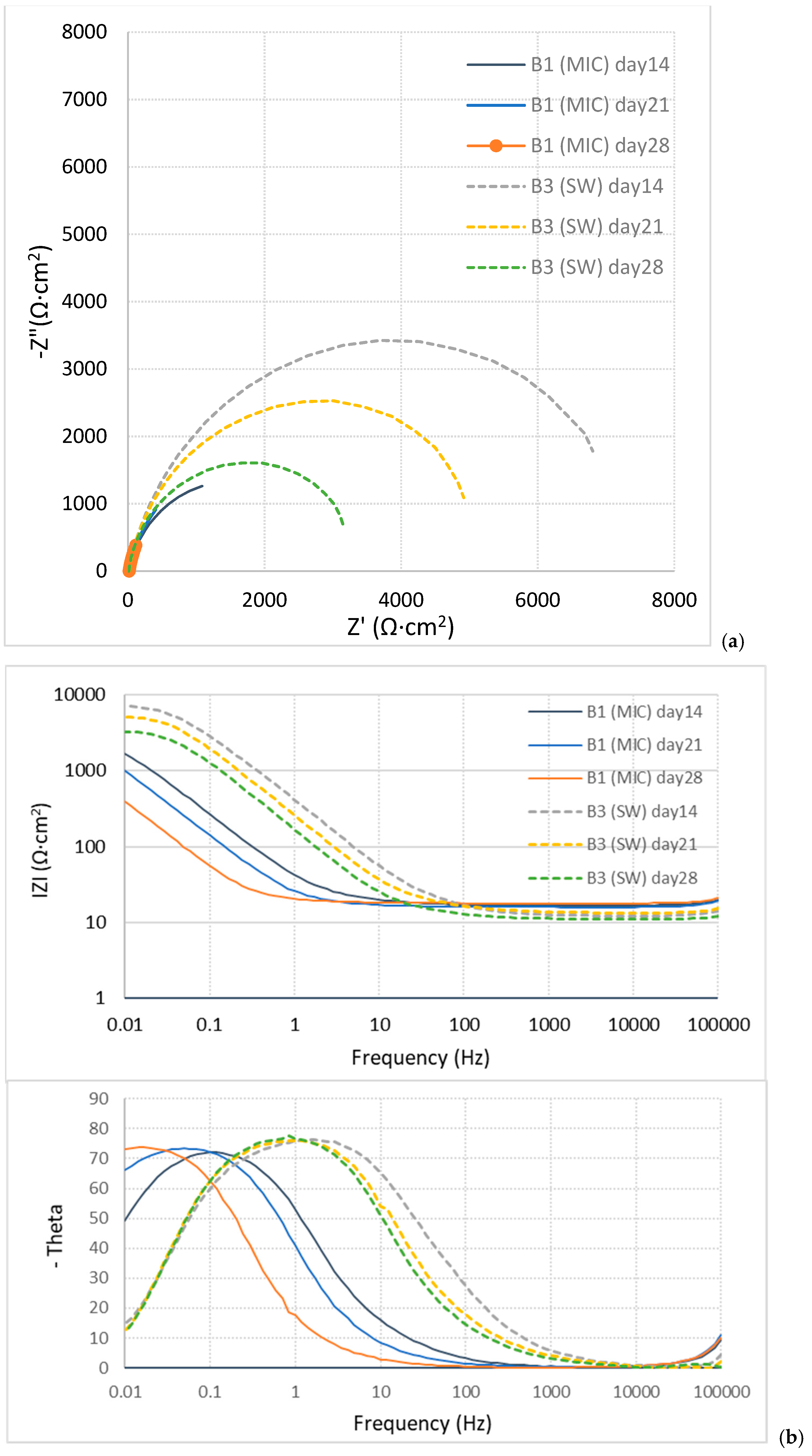
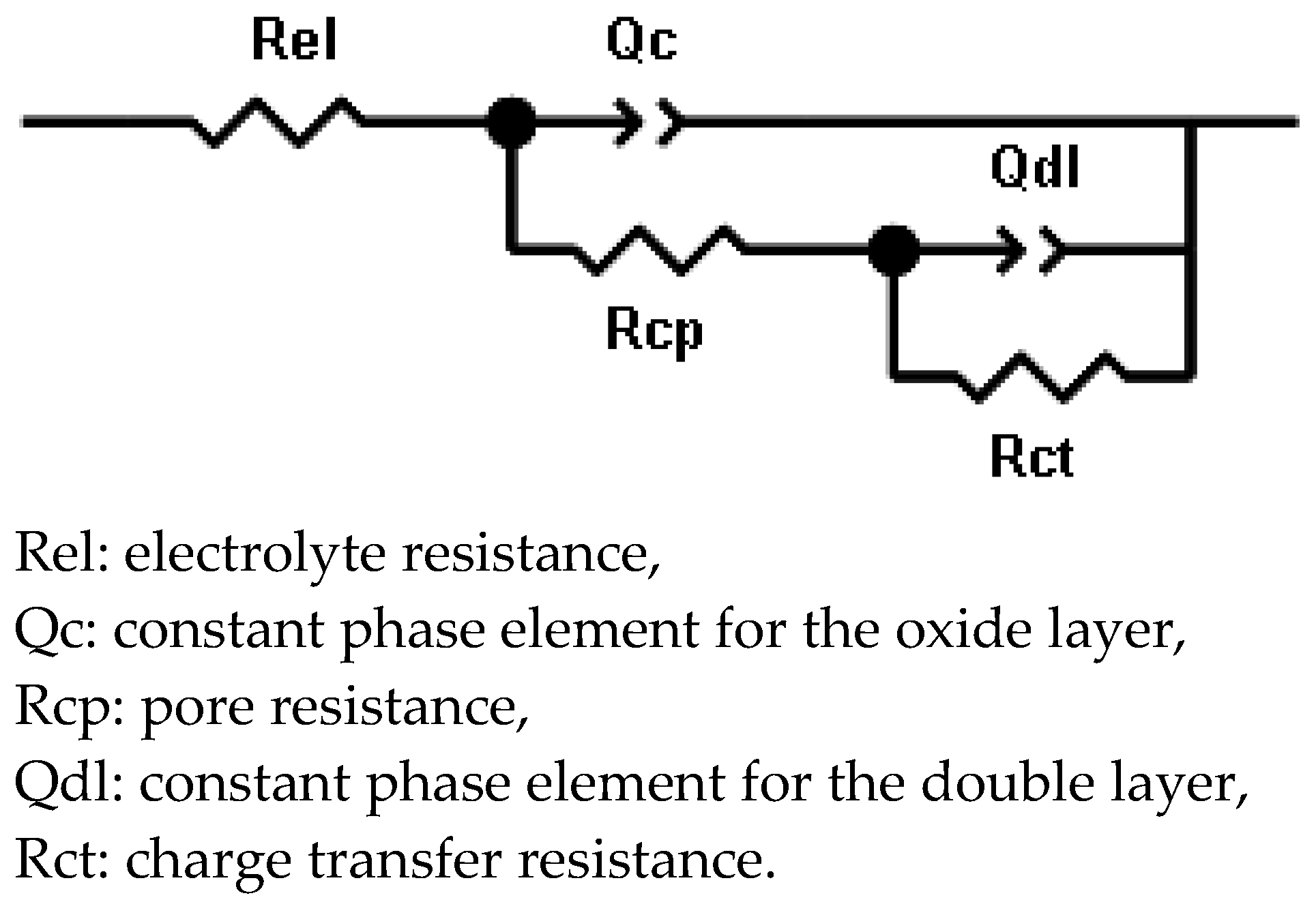
3.1.3. EIS Measurements
3.2. Surface Analysis
3.2.1. Epifluorescence Microscopy
3.2.2. Corrosion Morphology
Steel in Seawater without Bacteria
Steel in Seawater with Bacteria
3.2.3. Microstructure and Inclusions in the Steel
4. Discussion
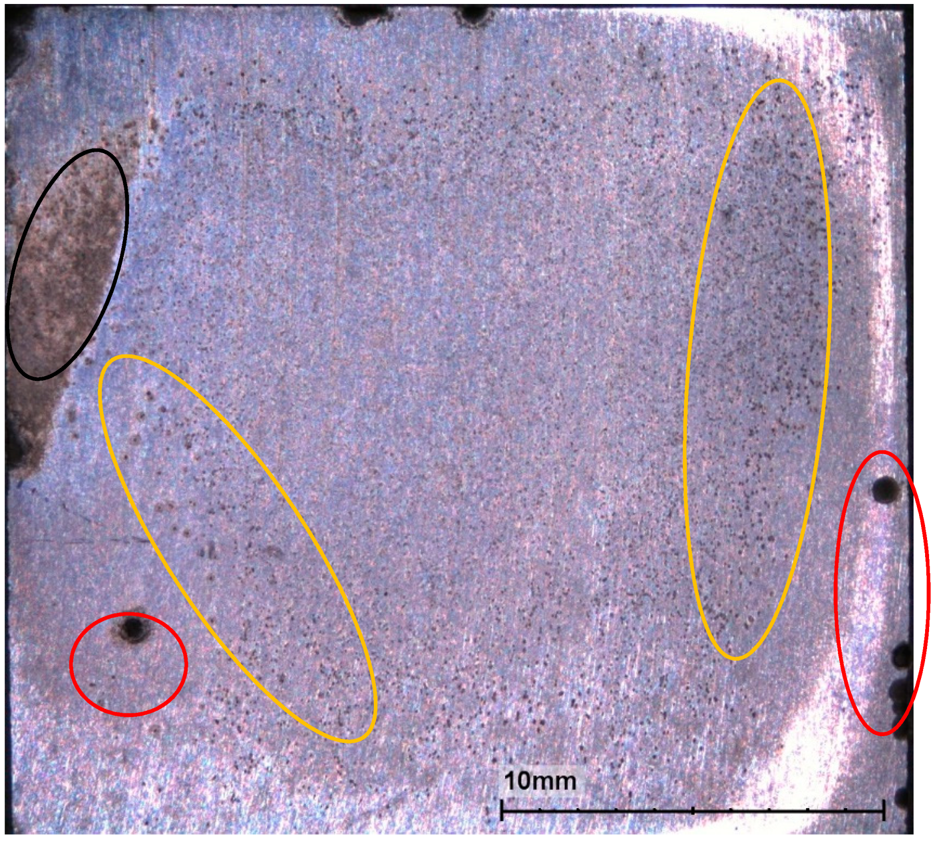
- (a)
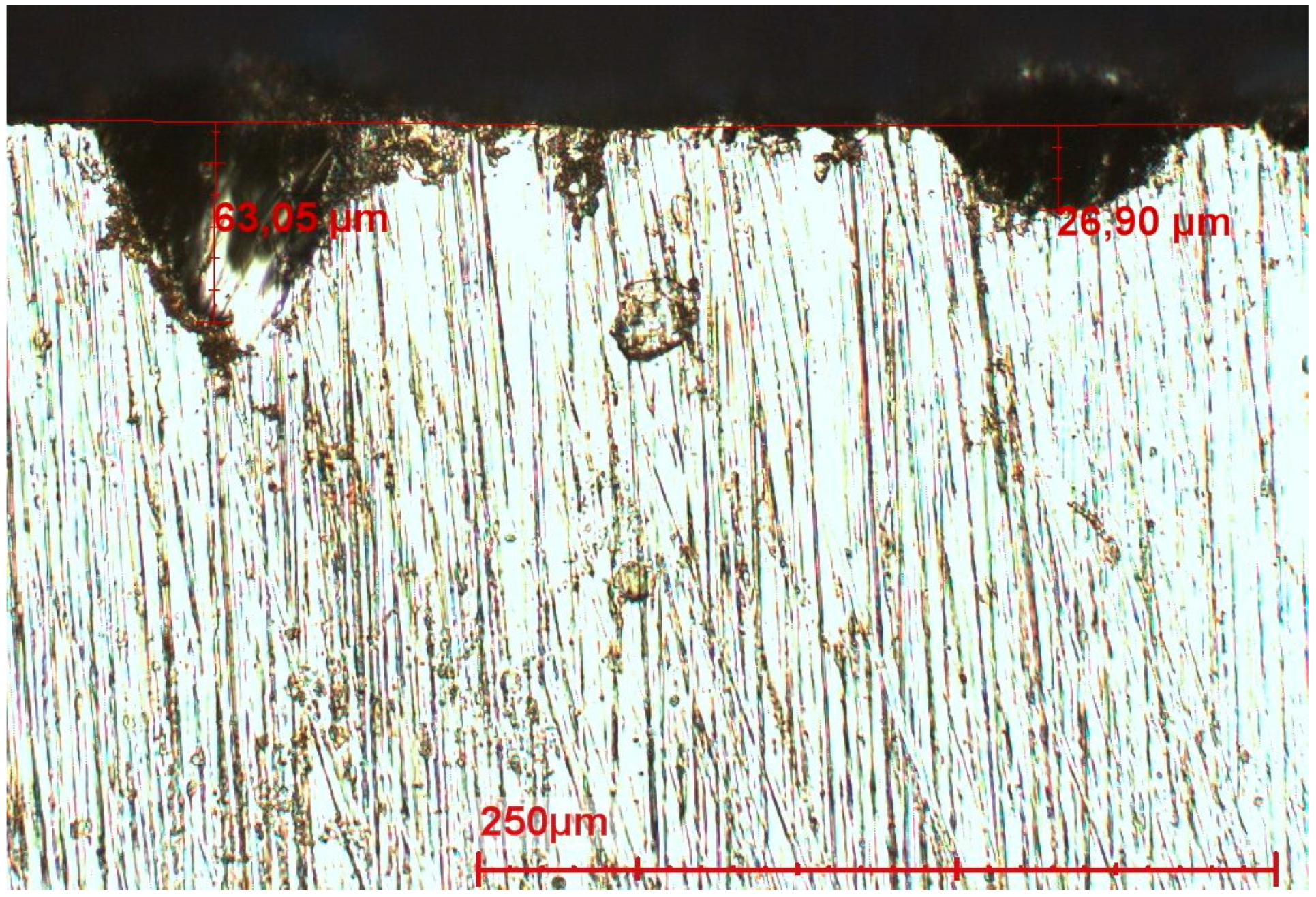
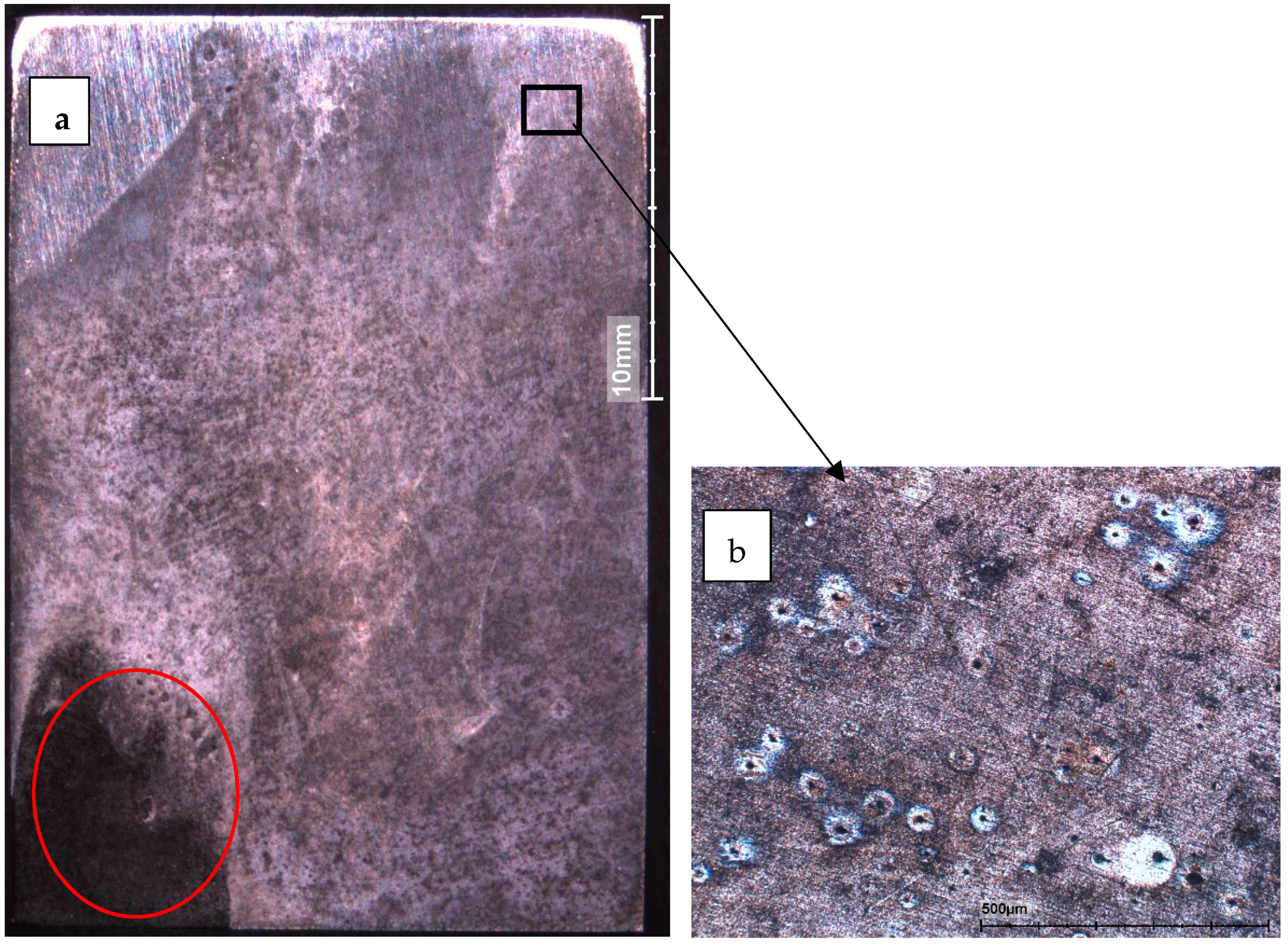
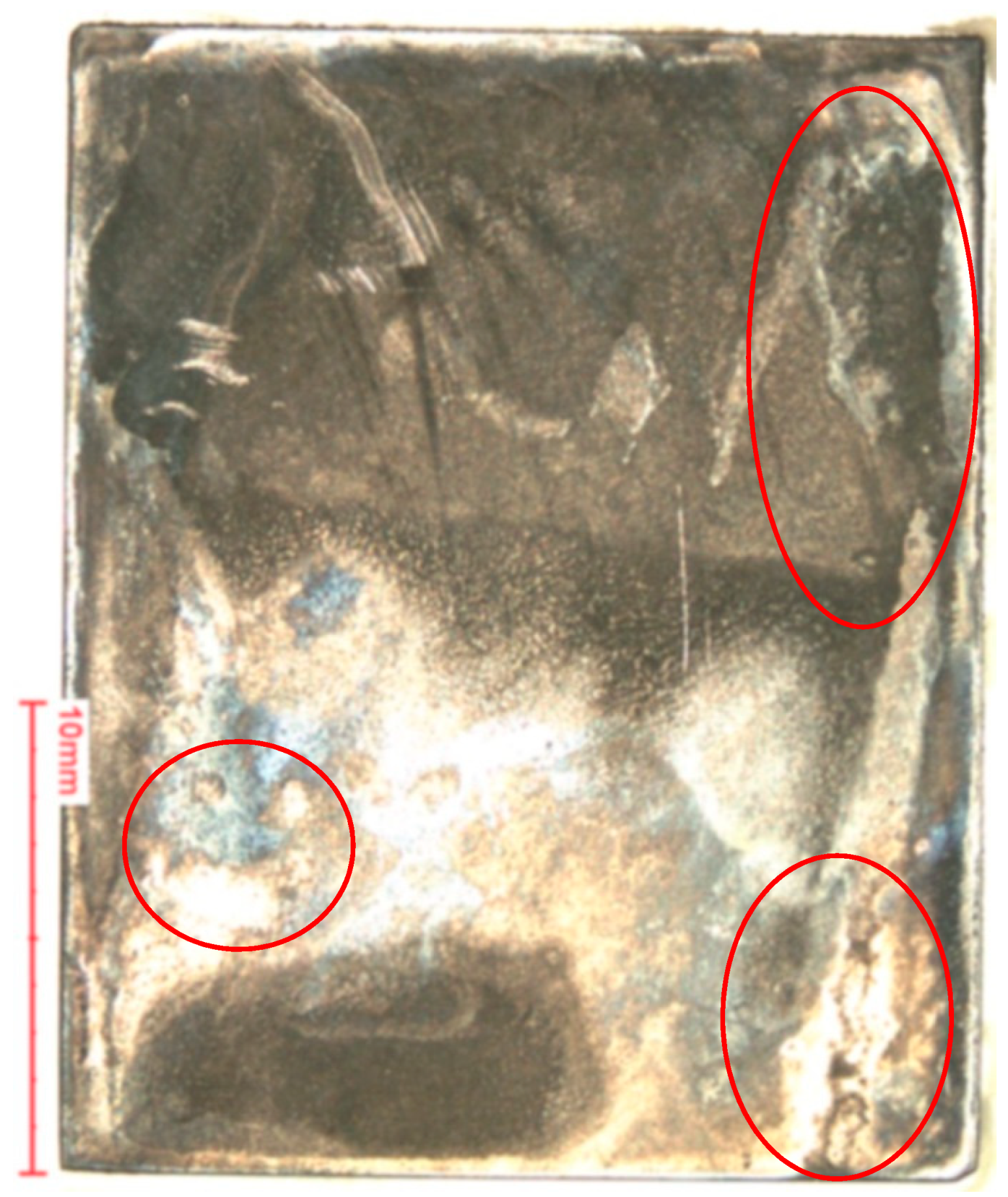
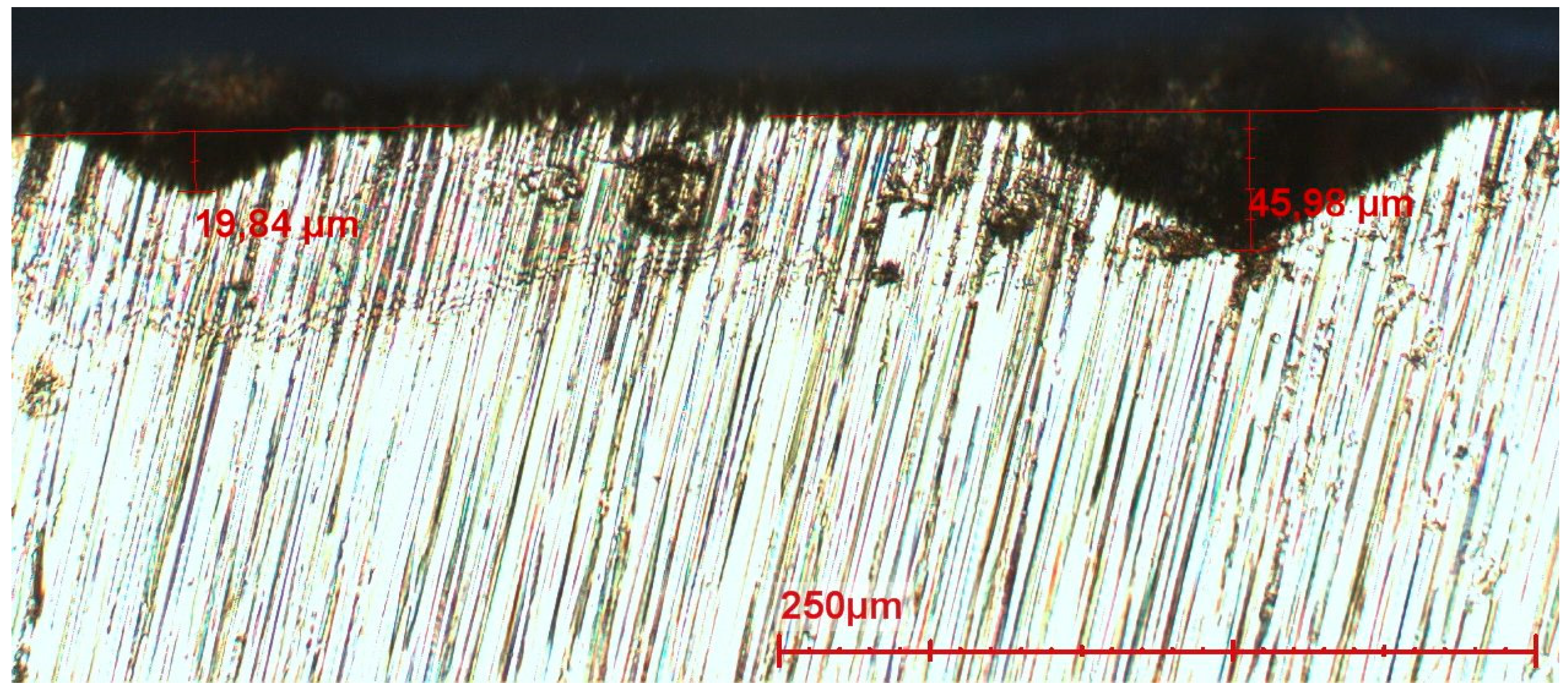
- Relatively small pits which occur in large areas of the steel. Local corrosion attacks initiate at defects such as the grain boundaries or inclusions. According to literature these “micro” pits are formed very quickly after immersion. Most of these pits reach the depth of 100–200 µm and then stop propagating [20,30]. Pits can continue their growth only under a layer of corrosion products or biofilms. The observed pits are the locations where anodic reactions occur, the rest of the surface being the cathodic part. Sometimes after the start of exposure, corrosion products are formed in the pits increasing the electrical resistance and inhibiting the access of oxidizing agents. Then the reactions stop and start elsewhere, but with lower driving forces.
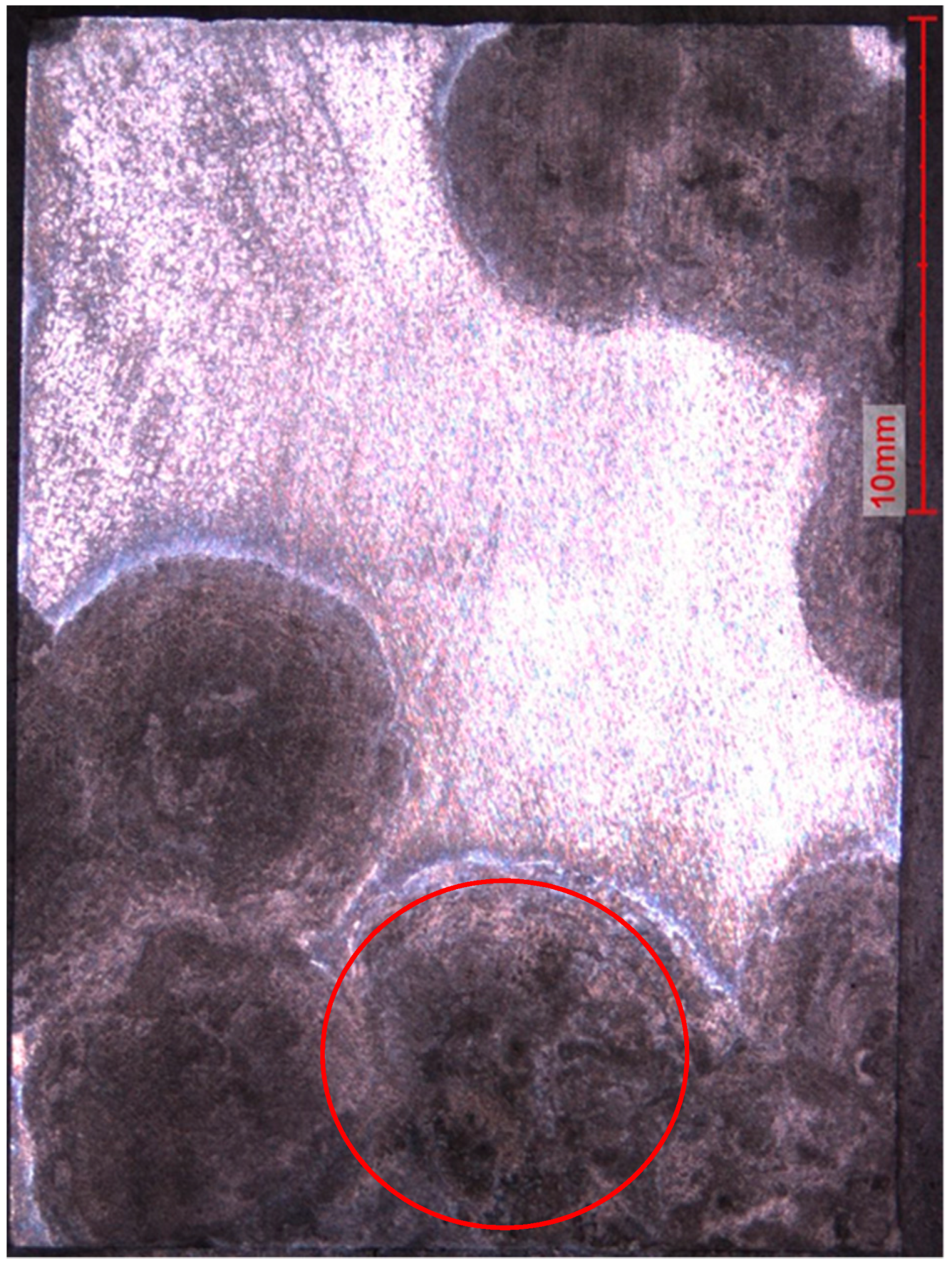
- (b)
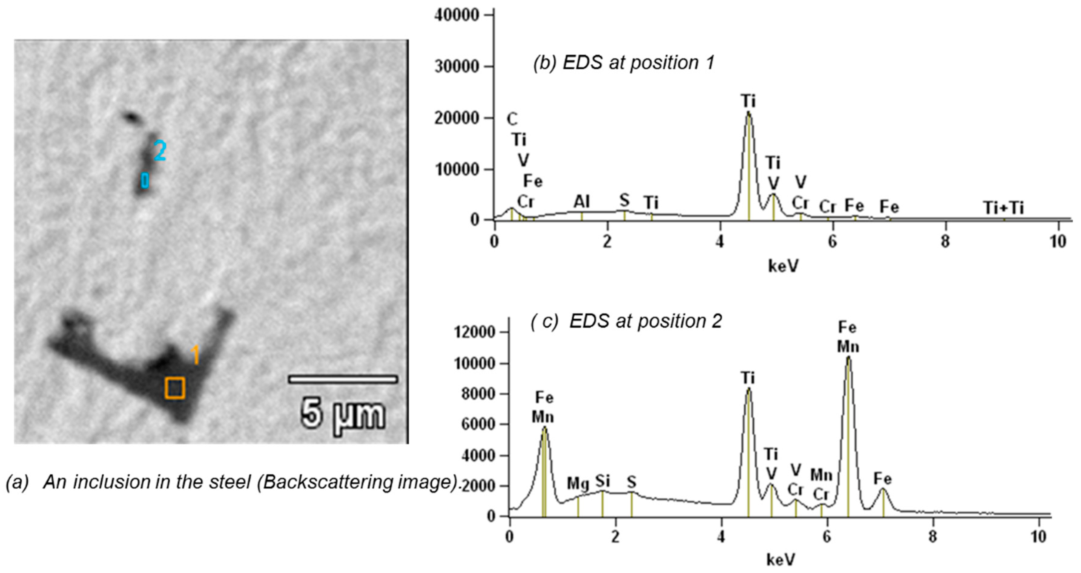
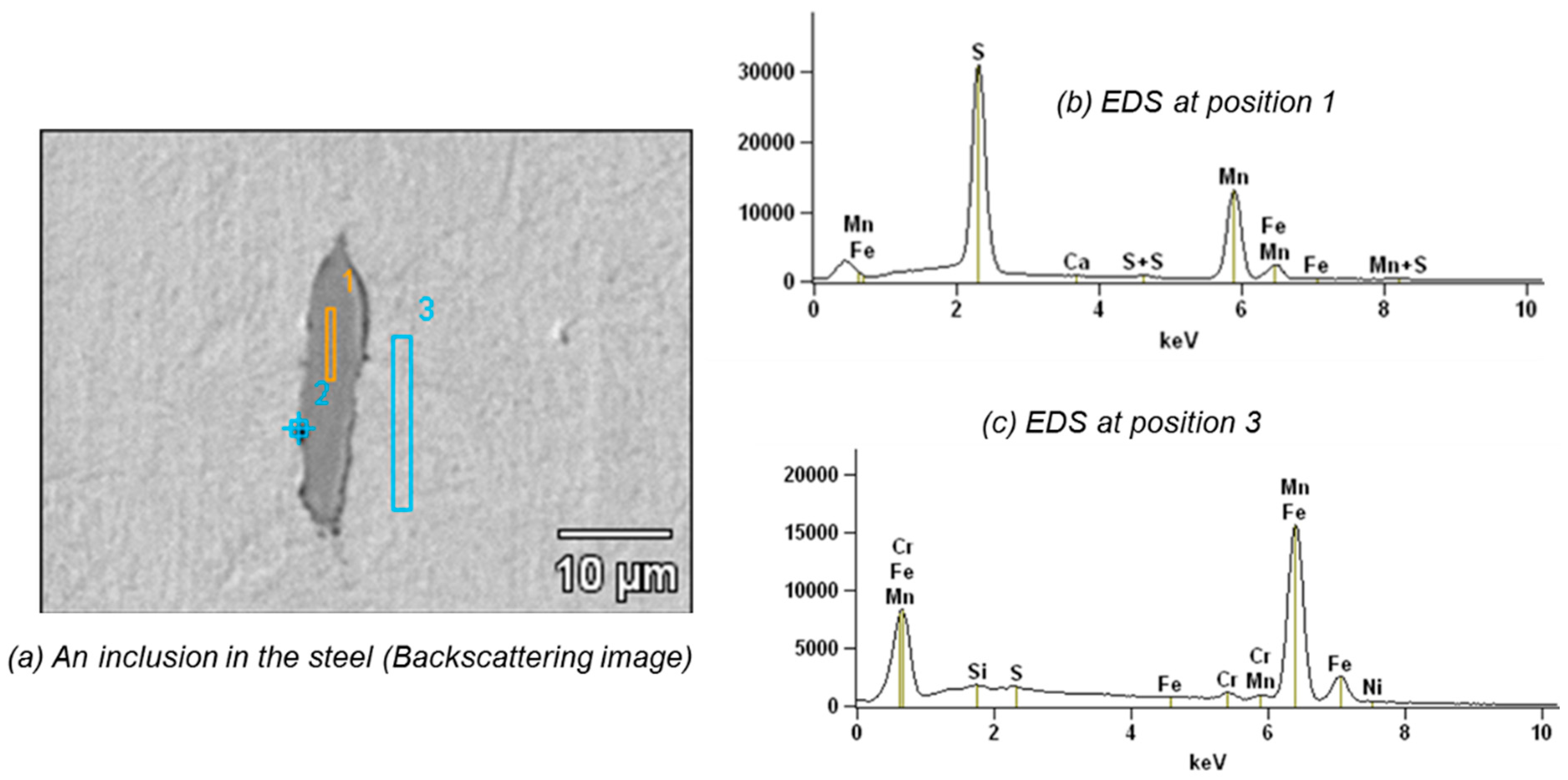
- A limited number of clearly larger pits is found on the surface of all samples. In contrast to the small pits described above, these pits are found in limited locations. These relatively large corrosion spots initiate from small pits and grow in depth and laterally due to high local driving forces such as local metallic inclusions. Relatively large inclusions are found in the steel (MnS and TiVCr, 5–20 µm, see Figure 18 and Figure 19); inclusions are known to have different potentials with regard to the matrix and cause local galvanic corrosion. Therefore, it is obvious that a link exists between the inclusions found and the large pits.
5. Conclusions
- (a)
- Localized corrosion has been found in the absence as well as in the presence of microorganisms, and occurs from the start of the exposure.
- (b)
- Inclusions of MnS and TiVCr have been detected in the R4 steel. These inclusions formed during the manufacture of the chain steel have a critical influence on the local corrosion attack.
- (c)
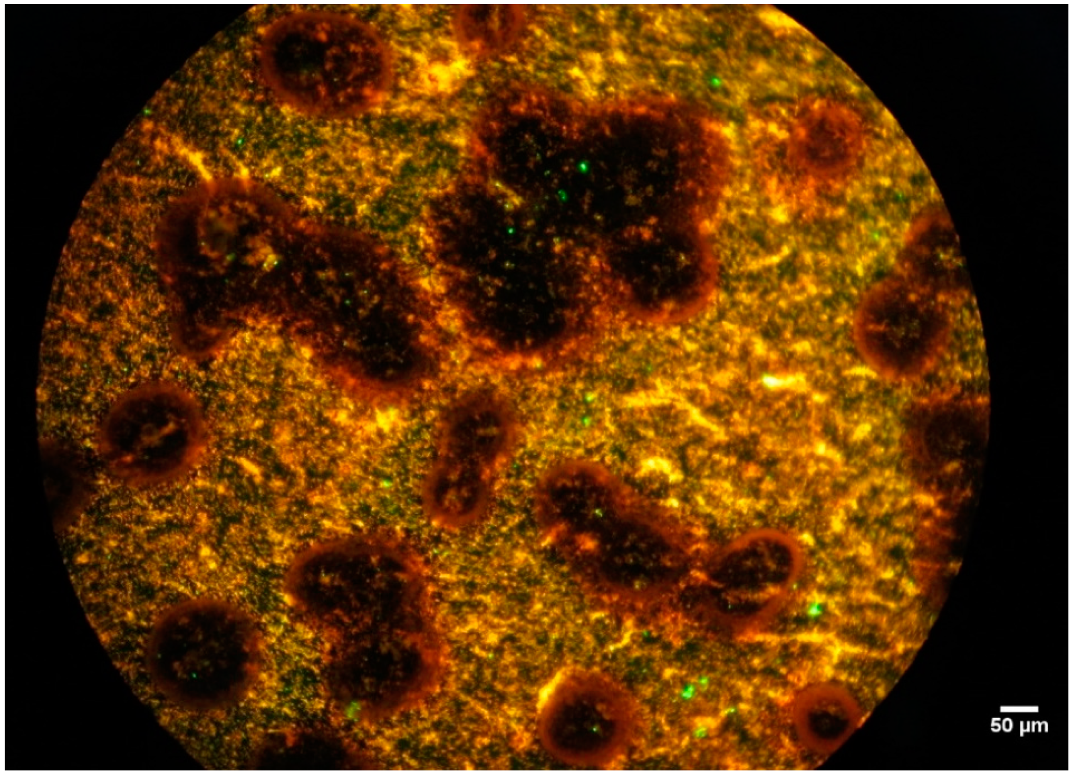
- With the addition of bacteria, already after 7 days of incubation an active biofilm was detected on the surface of the coupons with favoured locations in and around the pits.
- (d)
- The localized corrosion rate was as high as 0.82 mm/y in the SW in the presence of bacteria. In the case of local corrosion, applying uniform corrosion measurement techniques and formulas are not considered representative. This paper shows that representative areas have to be introduced to match physical results with the measurements.
Author Contributions
Funding
Institutional Review Board Statement
Informed Consent Statement
Data Availability Statement
Acknowledgments
Conflicts of Interest
References
- Ma, K.T.; Shu, H.; Smedley, P.; L’Hostis, D.; Duggal, A. A Historical Review on Integrity Issues of Permanent Mooring Systems; OnePetro: Houston, TX, USA, 2013. [Google Scholar]
- Fontaine, E.; Kilner, A.; Carra, C.; Washington, D.; Ma, K.T.; Phadke, A.; Laskowski, D.; Kusinski, G. Industry Survey of Past Failure, Pre-Emptive Replacements and Reported Degradations for Mooring Systems of Floating Production Units; OnePetro: Houston, TX, USA, 2014; p. 14. [Google Scholar]
- Zhang, X.; Hoogeland, M. Influence of deformation on corrosion of mooring chain steel in seawater. Mater. Corros. 2019, 70, 962–972. [Google Scholar] [CrossRef]
- Melchers, R.E.; Jeffrey, R.; Fontaine, E. Corrosion and the structural safety of FPSO mooring systems in Tropical waters. In Australasian Structural Engineering Conference 2012: The Past, Present and Future of Structural Engineering; Engineers Australia: Barton, Australian, 2012; p. 748. [Google Scholar]
- Fontaine, E.; Rosen, J.; Potts, A.; Ma, K.T.; Melchers, R. SCORCH JIP-Feedback on MIC and Pitting Corrosion from Field Recovered Mooring Chain Links. In Proceedings of the Offshore Technology Conference, Houston, TX, USA, 8 May 2014. [Google Scholar]
- Little, B.J.; Ray, R.I.; Lee, J.S. Microbiologically influenced corrosion of pilings. VTS Navig. Mooring Berthing 2013, 60, 69–71. [Google Scholar]
- GL Noble Denton. Microbiologically Influenced Corrosion of Mooring Systems for Floating Offshore Installations; HSE: London, UK, 2017.
- Veritas, D.N. Offshore Mooring Chain; Offshore Standard DNV-OS-E302; DNV: Bærum, Norway, 2013. [Google Scholar]
- ABS. Guide for the Certification of Offshore Mooring Chain. 2009. Available online: https://ww2.eagle.org/content/dam/eagle/rules-and-guides/current/survey_and_inspection/39_certificationoffshoremooringchain_2017/Mooring_Chain_Guide_e-May17.pdf (accessed on 11 October 2021).
- Vicinay. Haewene Brim Chain Accessment, Report. 2013. Available online: https://vicinayinnovacion.com/case-studies/ (accessed on 11 October 2021).
- Fontaine, E.; Potts, A.; Ma, K.T.; Arredondo, A.; Melchers, R.E. SCORCH JIP: Examination and Testing of Severely-Corroded Mooring Chains from West Africa. In Proceedings of the Offshore Technology Conference, Houston, TX, USA, 30 April 2012. [Google Scholar]
- DNVGL. Position Mooring, Offshore Standards. 2018. Available online: https://rules.dnv.com/docs/pdf/DNV/os/2018-07/dnvgl-os-e301.pdf (accessed on 11 October 2021).
- Shu, H.; Yao, A.; Ma, K.T.; Ma, W.; Miller, J. API RP 2SK 4th Edition-An Updated Stationkeeping Standard for the Global Offshore Environment. In Proceedings of the Offshore Technology Conference, Houston, TX, USA, 30 April 2018. [Google Scholar]
- Melchers, R.E.; Chaves, I.A.; Jeffrey, R. A Conceptual Model for the Interaction between Carbon Content and Manganese Sulphide Inclusions in the Short-Term Seawater Corrosion of Low Carbon Steel. Metals 2016, 6, 132. [Google Scholar] [CrossRef] [Green Version]
- Man, C.; Dong, C.; Xiao, K.; Yu, Q.; Li, X. The Combined Effect of Chemical and Structural Factors on Pitting Corrosion Induced by MnS-(Cr, Mn, Al)O Duplex Inclusions. Corrosion 2017, 74, 312–325. [Google Scholar] [CrossRef]
- Li, T.; Wu, J.; Frankel, G. Localized corrosion: Passive film breakdown vs. Pit growth stability, Part VI: Pit dissolution kinetics of different alloys and a model for pitting and repassivation potentials. Corros. Sci. 2021, 182, 109277. [Google Scholar] [CrossRef]
- Avci, R.; Davis, B.; Wolfenden, M.; Beech, I.; Lucas, K.; Paul, D. Mechanism of MnS-mediated pit initiation and propagation in carbon steel in an anaerobic sulfidogenic media. Corros. Sci. 2013, 76, 267–274. [Google Scholar] [CrossRef]
- Jeffrey, R.J.; Melchers, R.E. The effect of microbiological involvement on the topography of corroding mild steel in coastal seawater. In Proceedings of the CORROSION 2010, San Antorio, TX, USA, 14 March 2010. [Google Scholar]
- Melchers, R.E.; Moan, T.; Gao, Z. Corrosion of working chains continuously immersed in seawater. J. Mar. Sci. Technol. 2007, 12, 102–110. [Google Scholar] [CrossRef]
- Melchers, R.E. Pitting corrosion of mild steel in marine immersion environment-Part 1: Maximum pit depth. Corrosion 2014, 60, 824–836. [Google Scholar] [CrossRef]
- López-Ortega, A.; Bayón, R.; Pagano, F.; Igartua, A.; Arredondo, A.; Arana, J.; Gonzalez, J.J. Tribocorrosion behaviour of mooring high strength low alloy steels in synthetic seawater. Wear 2015, 338-339, 1–10. [Google Scholar] [CrossRef]
- Mansfeld, F.; Little, B. A technical review of electrochemical techniques applied to microbiologically influenced corrosion. Corros. Sci. 1991, 32, 247–272. [Google Scholar] [CrossRef]
- Webb, D.J.; Brown, C.M. Epi-Fluorescence Microscopy. In Cell Imaging Techniques; Taatjes, D.J., Roth, J., Eds.; Humana Press: Totowa, NJ, USA, 2012; pp. 29–59. [Google Scholar]
- Heyer, A. Microbiological Influenced Corrosion in Ship Ballast Tanks; Haveka Holding, B.V.: Alblasserdam, Zuid-Holland, The Netherlands, 2013; ISBN 978-90-820590-0-7. [Google Scholar]
- Uhlig, H.H. Corrosion and Corrosion Control, 2nd ed.; John Wiley & Sons Inc.: Hoboken, NJ, USA, 1971. [Google Scholar]
- Stern, M.; Geary, A.L. Electrochemical Polarization 1. Theoretical analysis of the shape and polarization curves. J. Electrochem. Soc. 1957, 104, 56–63. [Google Scholar] [CrossRef]
- van Westing, E.P.M.; Ferrari, G.M.; De Wit, J.H.W. The determination of coating performance with impedance measurements -I. Coating polymer properties. Corros. Sci. 1993, 34, 1511–1530. [Google Scholar] [CrossRef]
- Buchheit, R.G.; Cunningham, M.; Jensen, H.; Kendig, M.W. A Correlation between Salt Spray and Electrochemical Impedance Spectroscopy Test Results for Conversion-Coated Aluminum Alloys. Corrosion 1998, 54, 61–69. [Google Scholar] [CrossRef]
- Gu, T.; Jia, R.; Unsal, T.; Xu, D. Toward a better understanding of microbiologically influenced corrosion caused by sulfate reducing bacteria. J. Mater. Sci. Technol. 2018, 35, 631–636. [Google Scholar] [CrossRef]
- Butler, G.; Stretton, P.; Beynon, J.G. Initiation and growth of pits on high-purity iron and its alloys with chromium and copper in neutral chloride solutions. Br. Corros. J. 1972, 7, 168–173. [Google Scholar] [CrossRef]
- Khan, M.A.A.; Hussain, M.; Djavanroodi, F. Microbiologically influenced corrosion in oil and gas industries: A review. Int. J. Corros. Scale Inhib. 2021, 10, 80–106. [Google Scholar] [CrossRef]
- Blackwood, D.J. An Electrochemist Perspective of Microbiologically Influenced Corrosion. Corros. Mater. Degrad. 2018, 1, 5. [Google Scholar] [CrossRef] [Green Version]
- Little, B.; Blackwood, D.; Hinks, J.; Lauro, F.; Marsili, E.; Okamoto, A.; Rice, S.; Wade, S.; Flemming, H.-C. Microbially influenced corrosion—Any progress? Corros. Sci. 2020, 170, 108641. [Google Scholar] [CrossRef]


| QR4 | C | Mn | Si | P | S | Ni | Mo | Cr | Al | Cu | Sn | V | Ti | As |
|---|---|---|---|---|---|---|---|---|---|---|---|---|---|---|
| min. | 0.18 | 0.85 | 0.15 | 0.50 | 0.20 | 0.90 | 0.015 | 0.04 | ||||||
| max. | 0.24 | 1.20 | 0.35 | 0.020 | 0.015 | 0.80 | 0.40 | 1.25 | 0.040 | 0.25 | 0.030 | 0.10 | 0.015 | 0.025 |
| Samples | SW | SW + Bacteria (MIC) | Test Duration (Day) |
|---|---|---|---|
| P1, P2 | PDP | ||
| B1, B2 | LPR + EIS | 28 | |
| B3, B4 | LPR + EIS | 28 | |
| S5, S6 | LPR | 21 | |
| S8, S9 | LPR | 7 | |
| S10, S11 | LPR | 21 | |
| S12, S13 | LPR | 28 | |
| S14, S15 | LPR | 7 |
| NaCl | MgCl2 | CaCl2 | Na2SO4 | KCl | NaHCO3 | KBr | H3BO3 | NaF | SrCl2 | Yeast | Lactate |
|---|---|---|---|---|---|---|---|---|---|---|---|
| 23.93 | 5.07 | 1.15 | 4.01 | 0.68 | 0.197 | 0.099 | 0. 03 | 0.01 | 0.14 | 0.01 | 4.2 mL |
| Steel | Ec (V) | icorr (µA/cm2) | ba (mV/dec) | bc (mV/dec) | CR (mm/y) |
|---|---|---|---|---|---|
| P1 | −0.64 | 26 | 68 | 618 | 0.30 |
| P2 | −0.63 | 25 | 65 | 676 | 0.29 |
| Sample | Solution | Time (Day) | |Z| (Ω·cm2) | Theta |
|---|---|---|---|---|
| B1 | SW + bacteria | 14 | 1629 | −49 |
| 21 | 980 | −66 | ||
| 28 | 392 | −73.2 | ||
| B2 | SW + bacteria | 14 | 2268 | −40 |
| 21 | 478 | −74.6 | ||
| 28 | 460 | −73 | ||
| B3 | SW | 14 | 7036 | −14.7 |
| 21 | 5038 | −12.5 | ||
| 28 | 3227 | −14.9 | ||
| B4 | SW | 14 | 5093 | −12.3 |
| 21 | 3880 | −13 | ||
| 28 | 3275 | −16 |
| Sample | Time (Day) | Cc | n1 | Rcp | Cdl | n2 | Rct | χ2 (×10−4) |
|---|---|---|---|---|---|---|---|---|
| B1 (MIC) | 14 | 0.00227 | 0.893 | 15 | 0.00125 | 0.899 | 3210.8 | 0.6 |
| 21 | 0.00673 | 0.869 | 17 | 0.00211 | 0.9998 | 4328.6 | 1.2 | |
| 28 | 0.01239 | 1 | 3 | 0.01007 | 0.868 | 3624.8 | 3 | |
| B2 (MIC) | 14 | 0.00104 | 1 | 3 | 0.00052 | 0.808 | 3654 | 0.9 |
| 21 | 0.00754 | 0.931 | 4 | 0.01378 | 0.932 | 4216.5 | 8 | |
| 28 | 0.01590 | 0.997 | 7 | 0.00410 | 0.814 | 4477.5 | 1.8 | |
| B3 (SW) | 14 | 0.00020 | 0.88 | 39 | 0.00007 | 0.965 | 7825.5 | 4.5 |
| 21 | 0.00023 | 0.932 | 14 | 0.00018 | 0.922 | 5494.3 | 8 | |
| 28 | 0.00038 | 0.94 | 10 | 0.00030 | 0.93 | 3487.4 | 5.9 | |
| B4 (SW) | 14 | 0.00015 | 0.872 | 12 | 0.00019 | 0.943 | 5512.6 | 5.2 |
| 21 | 0.00021 | 0.922 | 12 | 0.00031 | 0.931 | 4222.6 | 4.4 | |
| 28 | 0.00043 | 0.931 | 11 | 0.00038 | 0.93 | 3569 | 3.6 |
| Sample | Condition | Time (Day) | Uniform Corrosion | Macro-Pits | Micro-Pits | Corrosion Products Affected Area | Intact Area | Maximum Pit Depth (µm) |
|---|---|---|---|---|---|---|---|---|
| B1 | MIC | 28 | - | 30 | 70 | - | - | 42 |
| B2 | MIC | 28 | - | 20 | 70 | - | 10 | 63 |
| B3 | SW | 28 | 30 | 10 | 50 | 10 | - | 46 |
| B4 | SW | 28 | 40 | 10 | 50 | - | - | 39 |
| Element | Si | S | Ca | Cr | Mn | Fe | Ni |
|---|---|---|---|---|---|---|---|
| Position 1 | 6.2 | 38.0 | 0.2 | 53.2 | 2.4 | ||
| Position 3 | 0.5 | 0.4 | 2.0 | 1.2 | 95.3 | 0.6 |
| Element | C | Mg | Al | Si | S | Ti | V | Cr | Mn | Fe |
|---|---|---|---|---|---|---|---|---|---|---|
| Point 1 | 9.1 | 0.1 | 1.0 | 75.0 | 8.6 | 3.5 | 2.7 | |||
| Point 2 | 0.2 | 0.3 | 0.5 | 24.6 | 1.7 | 1.8 | 1.2 | 69.7 |
Publisher’s Note: MDPI stays neutral with regard to jurisdictional claims in published maps and institutional affiliations. |
© 2022 by the authors. Licensee MDPI, Basel, Switzerland. This article is an open access article distributed under the terms and conditions of the Creative Commons Attribution (CC BY) license (https://creativecommons.org/licenses/by/4.0/).
Share and Cite
Zhang, X.; Noël-Hermes, N.; Ferrari, G.; Hoogeland, M. Localized Corrosion of Mooring Chain Steel in Seawater. Corros. Mater. Degrad. 2022, 3, 53-74. https://doi.org/10.3390/cmd3010004
Zhang X, Noël-Hermes N, Ferrari G, Hoogeland M. Localized Corrosion of Mooring Chain Steel in Seawater. Corrosion and Materials Degradation. 2022; 3(1):53-74. https://doi.org/10.3390/cmd3010004
Chicago/Turabian StyleZhang, Xiaolong, Nanni Noël-Hermes, Gabriele Ferrari, and Martijn Hoogeland. 2022. "Localized Corrosion of Mooring Chain Steel in Seawater" Corrosion and Materials Degradation 3, no. 1: 53-74. https://doi.org/10.3390/cmd3010004
APA StyleZhang, X., Noël-Hermes, N., Ferrari, G., & Hoogeland, M. (2022). Localized Corrosion of Mooring Chain Steel in Seawater. Corrosion and Materials Degradation, 3(1), 53-74. https://doi.org/10.3390/cmd3010004