Article

Interactions Between Business Cycles, Financial Cycles and Monetary Policy in South Africa

by
Malibongwe Cyprian Nyati
1,*,
Paul-Francois Muzindutsi
2 and
Christian Tipoy
2
1
Faculty of Economics and Finance, Tshwane University of Technology, Tshwane 0208, South Africa
2
School of Accounting, Economics and Finance, University of KwaZulu-Natal, Durban 4000, South Africa
*
Author to whom correspondence should be addressed.
Forecasting 2026, 8(3), 51; https://doi.org/10.3390/forecast8030051
Submission received: 22 February 2026 / Revised: 8 June 2026 / Accepted: 9 June 2026 / Published: 16 June 2026

Highlights

What are the main findings?
  • The financial cycle has become the main driver of fluctuations in the real economy.
  • The SARB can adopt financial stability as a secondary objective of monetary policy.
What are the implications of the main findings?
  • In stabilising the real economy, the SARB should also consider developments in the financial system. In stabilising the financial system, the SARB needs to consider fluctuations in the real economy.
  • A finance-augmented Taylor rule is more effective at stabilising both the real economy and the financial system than the traditional Taylor rule.

Abstract

This study set out to investigate the interactions between business cycles, financial cycles and monetary policy in South Africa. Explicitly, the study aims to examine the role of financial factors in business cycle models and the possibility of a unified macroeconomic framework in South Africa. Further, the study assesses the effects of demand shocks, supply shocks, interest rate shocks, and financial shocks on macroeconomic fluctuations. The study applied an analytical approach integrating the Generalised Method of Moments and System Generalised Method of Moments with a Structural New Keynesian Dynamic Stochastic General Equilibrium framework. Accordingly, it was concluded that the financial cycle plays a significant role in business cycle models and is a main driver of macroeconomic fluctuations in South Africa. Further, a unified macroeconomic framework for monetary policy analysis that links the financial system to the real economy in South Africa possibly exists. This study contributes to the South African Reserve Bank’s efforts by deepening understanding of the interactions between the financial system and the real economy and their implications for monetary policy in South Africa. By comparing the standard Taylor rule with a finance-augmented Taylor rule in a DSGE framework, the study helps answer the question of whether financial stability should be adopted as a second objective of monetary policy.

1. Introduction

Business cycle (BC) studies have been based on models that disregarded financial factors, mainly before the 2007–2009 global financial crisis (GFC). These models include the New Keynesian models (NKM) and the real business cycle (RBC) models [1,2]. Among others, the ever-changing nature of real indicators such as employment and unemployment rates, consumption expenditure, output, and prices, has been a principal focus in such studies. The dynamics of significant financial variables, viz., credit, house prices, equity, and spreads, were ignored in these studies [3]. Presently, however, several studies [4,5,6,7,8,9,10] have expressed interest in understanding the dynamic interactions and incorporation of financial factors in BC models. This, therefore, serves as proof that macroeconomists have not discarded financial factors in shaping their macroeconomic thought.
While an enormous number of studies have examined the interconnectedness of the financial and real sectors of the economy before the GFC, less attention was paid to financial shocks and financial factors as sources of BC fluctuations. Following the RBC literature, technological shocks have been at the forefront of views on the sources of business cycle fluctuations, particularly in developed countries. To an extent, financial factors were found to play little or no role in these fluctuations [3]. In developing countries like South Africa, factors such as low levels of human capital, the stance of structural policies and macroeconomic frameworks, and the lack of resource endowment, among others, have been at the forefront in shaping views on the sources of business cycle fluctuations [11,12,13].
After the GFC, however, macroeconomic activity thoughts expanded to consider the role of financial factors in BC fluctuations. This is revealed by the extant literature analysing business cycle models that feature financial factors [14,15]. For instance, in estimating a model with equity financing and debt, ref. [16] found that financial shocks played a substantial role in the observed dynamics of real and financial variables. Further, ref. [17] found that financial shocks affecting leverage sectors accounted for a larger share of the output collapse during the Great Depression. Recently, financial shocks have been found to be the main cause of recurrent oscillations and to have substantial negative effects on economic outcomes [see [17]]. Similar contributions are also found in [9,14,15,18], among others.
Due to the robust arguments about the nexus between the financial system and the real economy found in both empirical and theoretical studies, especially in the aftermath of the GFC. Presently, there is a near consensus that financial cycles and financial factors are a principal source of BC oscillations [3,19]. As a result, scholars need to incorporate the impact of financial cycles and financial factors when configuring business cycle models. As imperative as this is, and as it partly informs the South African Reserve Bank (SARB) research agenda. According to the authors’ knowledge, few, if any, studies have adopted a composite index to measure the financial cycle and its association with the BC and MP within an amalgamated macroeconomic framework for South Africa. This study, therefore, addresses an important avenue of research. The findings of this study are intended to provide a directional understanding of the interactions among BC, FC, and monetary policy. They will further respond to the question of what informs BC fluctuations and whether the SARB can adopt financial stability as a secondary objective.
The literature on BC studies before the GFC focused only on macroeconomic models that did not consider the impact of financial factors [1,2]. The common view among these studies was that technological shocks were the only known basis of BC oscillations, to the extent that they were found to explain a considerable degree of variation in BCs [20]. Another common feature of these studies was that they were all based on general equilibrium models. However, when structural vector autoregressive analyses were conducted, they indicated other disturbances as sources of BC fluctuations. Little to no evidence was found in support of technological shocks as drivers of output fluctuations [21,22,23,24].
In line with the structural VAR literature, studies in developing countries have identified other disturbances as the main drivers of BC oscillations. For example, in the empirical analysis of macroeconomic fluctuations reported in [11], it was concluded that factors such as low levels of human capital, structural policies, and the stance of the macroeconomic framework, among others, play a pivotal role as sources of BCs in South Africa. The authors also noted that the world interest rate and the money supply accounted for 18% and 30% of output fluctuations, respectively, and that exchange rates fluctuated mostly in response to changes in monetary policy. Therefore, several studies [21,22] on BC fluctuations, especially those conducted before the GFC, have pointed to other factors as the main drivers of BC oscillations; however, little or no evidence was provided on the role of financial factors in shaping these oscillations.
However, the aftermath of the GFC and the costs imposed on different countries’ economies led to an expansion of views on the sources of BC oscillations to account for the effects of financial factors. It has also led to amplified interest in studying the financial aspects of the BC [23,24,25,26,27,28,29,30,31,32]. For instance, in ref. [33], financial factors were utilised to augment the standard monetary DSGE model. Using euro area and United States data, it was concluded that a new financial-sector shock explained a large portion of BC oscillations. Correspondingly, ref. [34] utilised bank production functions to augment the standard BGG model. It was shown that macroeconomic fluctuations were intensified by financial shocks coming from both the demand and supply sides.
Further, a model was developed in which equity financing and debt played explicit roles in examining the effects of financial shocks on the observed oscillations of financial and real variables. The evidence obtained showed that such financial shocks contributed significantly to fluctuations in real and financial variables [16]. Furthermore, a DSGE model was estimated by [17], in which bank losses triggered a recession. The results showed that two of the three components of the output breakdown during the Great Depression were due to other financial shocks affecting leveraged sectors, as well as redistribution. Similar findings are also reported in other studies, such as [18,30,35,36]. These authors also considered disturbances originating in the financial sector and proposed that they constitute a substantial portion of the factors driving BC oscillations.
Recently, ref. [37] utilised a penalty approach within a Structural VAR framework to study interactions between real and financial variables. The empirical evidence indicated that adverse macroeconomic outcomes arise from various financial shocks. Further, these shocks are not new; they have an important cyclical source dating back to the 1980s. Most recently, ref. [9] developed a monetary DSGE model to study which financial shocks drive the BC. The authors found that sentiment shocks generated plausible BC responses and accounted for 20% of fluctuations in investment and employment. In general, while an enormous amount of work has been conducted on this topic, this is mainly biased towards developed nations. In developing countries such as South Africa, this topic remains largely unexplored, and the literature has yet to discover its importance.
The extant literature reviewed above has strongly debated the importance of financial factors as sources of BC fluctuations and the need to incorporate financial factors and financial shocks into BC models (Ajello, Goldberg et al. 2018) [9]. To date, there is increasing consensus that financial factors and financial shocks possess significant information content regarding BC fluctuations. Therefore, in the configuration of BC models, scholars, academics, central bankers, and the public must ensure that the impact of these financial shocks and/or factors is incorporated. Failure to do so might lead to inconclusive results, hinder proper policy initiations and threaten the credibility of the central bank [see [3,9,14,15,17,18,23,34,37,38]]. To date, the South African Reserve Bank’s research agenda has expanded to include analyses of interactions between financial and real indicators, with the aim of understanding the multilateral interactions between macroprudential and monetary policies.
The literature on South Africa remains scant in response to the SARB’s agenda of understanding the interactions between macroprudential and monetary policies. The present study contributes to and responds to this initiative by investigating the interactions among BCs, FCs, and monetary policy in South Africa within a unified macroeconomic framework. The aim is to ascertain the direction of the relationship, assess the possibility of a unified macroeconomic framework, and determine whether the Reserve Bank can take on a second objective. This is achieved by analysing the model’s stability when the FC variable is embedded as a monetary policy target.
The rest of the paper is organised as follows. Section 2 presents a variant of the four-equation New Keynesian macroeconomic framework and the results of the interactions among the variables of interest derived from the framework, estimated using the Generalised Method of Moments and a Multiple-Equation Generalised Method of Moments. Section 3 presents a Dynamic Stochastic General Equilibrium (DSGE) model, its parameter calibration, simulations, and model inferences. Section 4 concludes the paper with a summary and conclusion.

2. Interactions of Business Cycles, Financial Cycles and Monetary Policy

2.1. Theoretical Framework on the Interactions Among BCs, FCs, and MP

Our conceptual framework encompasses the traditional three-equation New Keynesian framework, which is extended with a financial cycle equation. As a result, instead of estimating a three-equation model, the present article estimates a four-equation model featuring a New Keynesian IS curve, a New Keynesian Phillips curve, an augmented Taylor rule, and a financial cycle equation capturing the behaviour of the financial system.

2.1.1. The Extended Hybrid IS Curve

As an initial step, we build on the analyses of [39] and extend the traditional IS curve equation by incorporating the composite financial cycle index variable (CFCI) into the aggregate demand function. The estimated IS curve, featuring both forward- and backward-looking components of aggregate demand as well as a financial cycle, is given as follows:
y t = μ E t y t + 1 + α 1 y t 1 + α 2 y t 2 + β 1 ( r t E t π t + 1 ) + β 2 C F C I t + ε t y
where   y t is the output gap (measured as the deviation of real GDP from potential output), r t E t π t + 1 shows the real interest rate, C F C I t shows the composite financial cycle index, which is an improved version of the South African financial cycle (FC) and ε t y ~ i i d .   N ( 0 ,   σ y 2 ) is a demand shock [39]. The same IS curve is incorporated into the four-equation model to analyse the possibility of a unified macroeconomic framework.

2.1.2. The Phillips Curve

The Phillips Curve considered in this analysis features both forward- and backward-looking components of inflation, in addition to the standard explanatory variable, the output gap. The following equation illustrates this:
π t = β 1 E π t + 1 + ( 1 β 1 ) π t 1 + β 2 y t + ε t π
where the coefficient values of β 1 and ( 1 β 1 ) are used to capture the extent of forward and backwards-looking elements of inflation, respectively; y t is the output gap and ε t π   ~ i i d .   N ( 0 ,   σ π 2 ) is a supply shock [40].

2.1.3. The Financial Cycle

The equation used to capture the evolution of the financial cycle, as motivated by the stylised facts of the financial system, is given as follows:
C F C I t = θ 1 C F C I t 1 + θ 2 y t + θ 3 r t + ε t C F C I
where the coefficient θ 1 captures the persistent nature of the financial cycle, θ 2 capture the procyclical nature of the CFCI, θ 3 captures the effect of monetary policy on the CFCI and ε t C F C I   ~ i i d .   N ( 0 ,   σ c f c i 2 ) is the CFCI shock. As the financial cycle typically exhibits considerable persistence and co-movement with the BC, the coefficients θ 1 and θ 2 are expected to have positive signs. The sign of the coefficient θ 3 is expected to be negative because an increase in the interest rate is associated with a downturn in the financial cycle [3].

2.1.4. The Monetary Policy Rule

As prevalent in the literature, it is assumed that the central bank sets the nominal interest rate in accordance with a forward-looking conventional Taylor rule. This includes interest rate smoothing and systematic responses to inflation and the output gap, as given by the following equation:
r t = 0 + 1 π t + k + 2 y t + p + i = 1 p ρ i r t i + ε t r
where ρ 1 is the interest rate smoothing parameter, 1 and 2 show the preferences of the central bank with respect to inflation and output gap stabilisation, ε t r ~ i i d .   N ( 0 ,   σ r 2 ) is an exogenous monetary policy shock [3,41,42].

2.2. Methodology on the Interactions Among BCs, FCs, and MP

The analysis proceeds in four stages. First, a two-step Markov Switching Dynamic Factor Model in state-space form is used to construct the CFCI from 13 financial time series, thereby capturing the latent financial cycle. Second, the constructed CFCI is treated as an observable variable and incorporated into a four-equation New Keynesian framework estimated by MEGMM. Third, the estimated parameters of the financial cycle equation, specifically: κ c f c i = 1.092 and ρ c f c i = 0.924 , are imported into a calibrated DSGE model, preserving the empirical discipline from stage two. Fourth, the DSGE model is used for policy counterfactual analysis, comparing a standard Taylor rule with an augmented Taylor rule.
The hypotheses we intend to evaluate here are such that: 1. financial factors and financial shocks play a significant role in shaping BC oscillations; 2. there exists a possible unified macroeconomic framework in South Africa that features both the financial system and the real economy; and 3. can the SARB adopt financial stability as a fully-fledged objective while still delivering price stability? This section tests the abovementioned hypotheses using a four-equation New Keynesian framework detailed above.
An extensive database was constructed using monthly time series of financial and economic variables for South Africa spanning the period 2000M01 to 2018M12. This period is informed by the availability of FC data and the desire to focus on the periods before, during and after the 2007–2009 GFC. While the literature has not yet reached a consensus on the time series indicators to be utilised in measuring FCs, this article follows the footsteps of [3,43,44] among others, in measuring the CFCI. Accordingly, this article adopted thirteen (13) monthly financial time series variables to measure the CFCI. The specific CFCI variables adopted include real broad effective exchange rate, house prices, All Share Price Index, long-term government bond yields, 10-year government bond yields, 5-year government bond yields, total credit to the private non-financial sector, the nominal effective exchange rate, and the Treasury bill rate.
All CFCI variables were converted to a single unit of measure using the Min–Max normalisation technique, as per the norm for constructing indices. The Min–Max normalisation procedure helps convert the variables to a common range of 0 to 1. This allows us to interpret our composite index with ease: an increase indicates improved financial conditions, while a decrease indicates deteriorating financial conditions [3]. Since our index lies between 0 and 1, it will be interpreted here as a unit increase or decrease. The Min–Max method is as follows:
V i t = V i t M i n ( V i ) M a x ( V i ) M i n ( V i )  
where V i t is the value of variable i during period t ; M i n ( V i ) and M a x ( V i ) denotes the minimum and maximum values observed during the sample period, respectively; and V i t shows the normalised values of the variable. A major downside of this procedure is that it does not handle outliers very well. As a result, the authors manually normalised each variable, ensuring that all variables were within the required ranges and that no outliers existed. Once all variables are in a single unit of measure, the methodology outlined below is used to measure both the FC proxy index and the CFCI.
This article proposes a two-step Markov Switching Dynamic Factor Model in state-space form, first proposed by [45], as a suitable model for studying the South African financial cycle. The analysis follows the same specification of [46] and assumes that the growth rate cycle has two states, viz., a downturn and an upturn. Financial sector activity, in this case, is represented by an unobservable factor extracted from an amalgamation of several observable variables.
The model is divided into two equations: the first defines a factor model, and the second defines a Markov Switching Dynamic Regression model for the common factor. Precisely, the first equation shows each series in the information set decomposed into the sum of a common component and an idiosyncratic component as follows:
y t = γ f t + z t
where y t is an N × 1 vector of economic indicators, f t is a univariate common factor, z t is an N × 1 a vector of idiosyncratic components that is uncorrelated with f t at all leads and lags, and γ is an N × 1 vector. The requirement of this equation is that all variables be stationary, i.e., all individual indicators be detrended, and only their cyclical components are used for the analysis at hand [47].
The second equation defines the Markov Switching model of [48]. This model can mark time. In terms of this model, a latent random variable s t governs the state or regime, with s t = 0 indicating low or negative growth and s t * = 1 indicating high or positive growth. Two states indicating positive and negative average growth rates are sufficient to mark turning points, since y t < 0 indicate a downturn and y t > 0 an upturn (Bosch and Ruch, 2013) [49].
Markov switching regression models allow parameters to vary across unobserved states. In the simplest case, this model can be expressed as a Markov Switching Dynamic Regression model (MSDR) with a state-dependent intercept term as follows:
y t = μ s t + ε t
where μ s t is the parameter of interest, μ s t = μ 1 when s t = 1 , and μ s t = μ 2 when s t = 2 . MSDR models allow quick adjustment after the process changes state. These models are often used to model monthly or higher-frequency data. The MS-DFM model can be estimated in either a one- or two-step process [47]. The main limitation of the one-step estimation procedure is that it can only be estimated with a smaller set of variables. This approach was found to be too constrained for this analysis. As a result, this article resorted to using a two-step estimation approach as follows:
The first step involves extracting a common factor f t from an amalgamation of a large set of financial variables according to Equation 6 above, without considering its Markov switching dynamics. To this end, this article utilises both a Dynamic Factor Model and Principal Component Analysis (PCA), considering that the first factor or principal component, f ^ t , provides a good approximation of the common factor. In this context, the article estimated the following Equation (9) to develop a CFCI for South Africa:
( f t f t 1 ) = ( θ 1 θ 2 1 0 ) ( f t 1 f t 2 ) + ( V t 0 )
(   R B E E R t H P t A S P t G B 10 Y t G B 5 Y t T C P F S t L T G B Y t N E E R t M 1 t M 2 t M 3 t T B I L L t I L R t   ) = ( γ 1 γ 2 γ 3 γ 4 γ 5 γ 6 γ 7 γ 8 γ 9 γ 10 γ 11 γ 12 γ 13     ) f t + ( ε 1 t ε 2 t ε 3 t ε 4 t ε 5 t ε 6 t ε 7 t ε 8 t ε 9 t ε 10 t ε 11 t ε 12 t ε 13 t   )
The second step estimates the parameters of an MSDR using maximum likelihood. This was aimed at fitting a univariate model (as seen in Hamilton, 1989) [48] to the estimated factor   f ^ t , which is treated as an observed variable. To identify the CFCI peaks and troughs, the article follows [50] Krznar (2011). A CFCI peak is identified in period t if financial sector activity was in an upturn during period t 1 and the filtered probability P r ( s t + 1 = 1 | t 1 , p , q , μ 1 , μ 2 σ 2 ) 0.5 . A trough is defined in period t if financial sector activity was on a downturn in period t 1, and the filtered probability P r ( s t + 1 = 1 | t 1 , p , q , μ 1 , μ 2 σ 2 ) 0.5 . Since the MS-DFM-SS is a model-based approach, it can select appropriate variables to construct the final composite index.
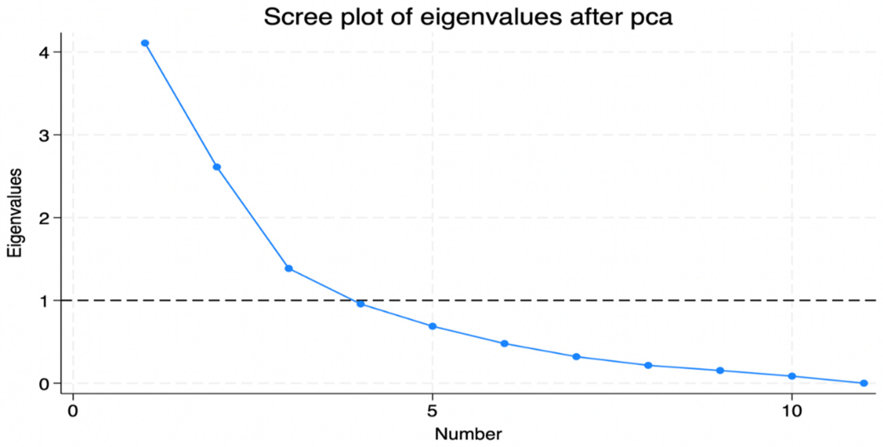
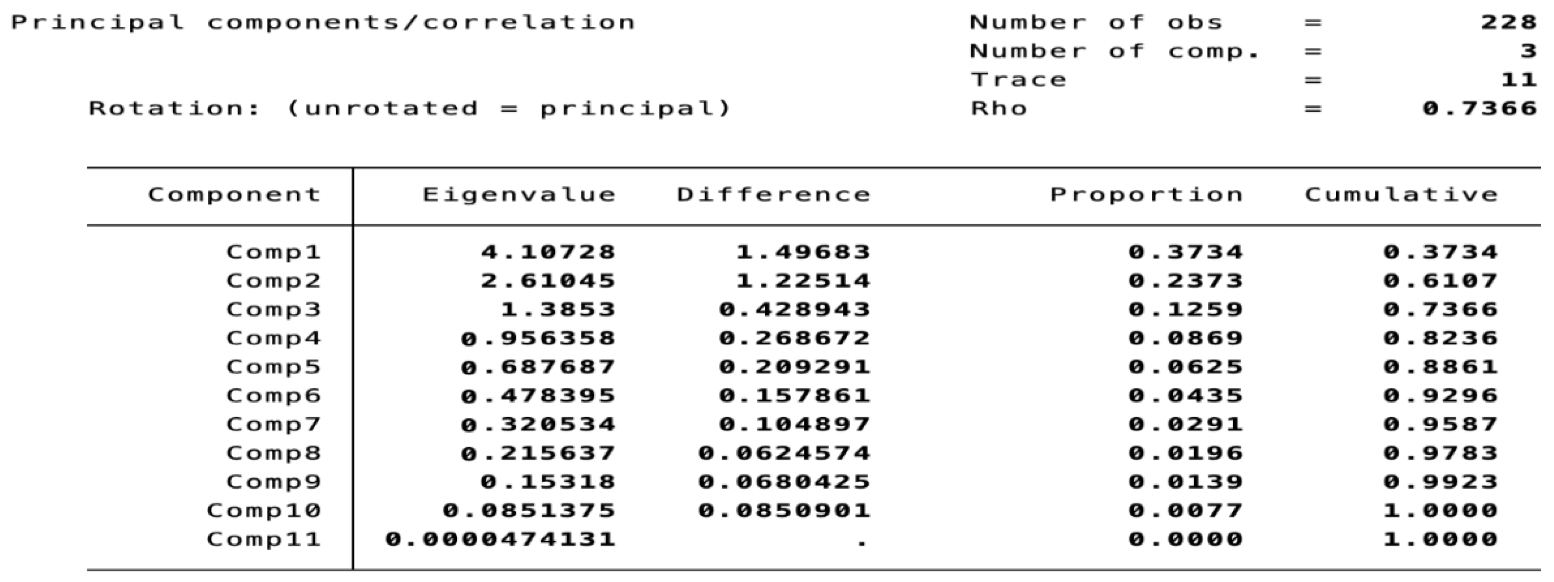
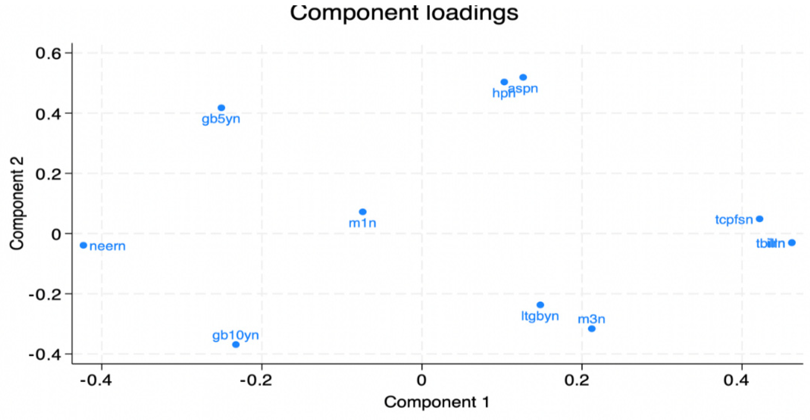
Accordingly, after estimation, 11 of the 13 variables initially suggested were retained for constructing the financial composite index. The first factor, or principal component, was selected because it explained about 37% of the total variance (see Figure A2, Figure A3 and Figure A4 in Appendix A). The constructed CFCI, using the methodology defined above, is shown in Figure 1.
Figure 1 shows the CFCI relative to the ±1.5 standard deviation boundaries. The CFCI accurately captures both periods of instability and imbalance. The main events, such as the 2001 rand crises and the 2007–2009 GFC, appear to be well captured by the index. Further, the index indicates that both upward (potential build-up of imbalances) and downward (manifestation of instabilities) phases are meaningful signals of financial instability. Subsequently, Table 1 presents the turning points of the CFCI obtained from the filtered probabilities of the MSDR model. Based on the rule for turning point identification in view of filtered probabilities, two peaks of the CFCI were identified: one in May 2003 and another in September 2008. These are the highest points that mark the end of expansion and the beginning of contraction periods in financial activity.
We further identified two troughs of the CFCI: one in January 2006 and another in June 2011. Again, these points mark the end of the deterioration in financial activity and the transition to expansion. Accordingly, the average length of the upturn phases exceeds that of the average length of the downturn phases. Further, the overall length of the CFCI (7.2 years) exceeds that of the business cycle (7.0 years). These results are in line with those of [51], who posited that the financial cycle is usually longer than the business cycle.
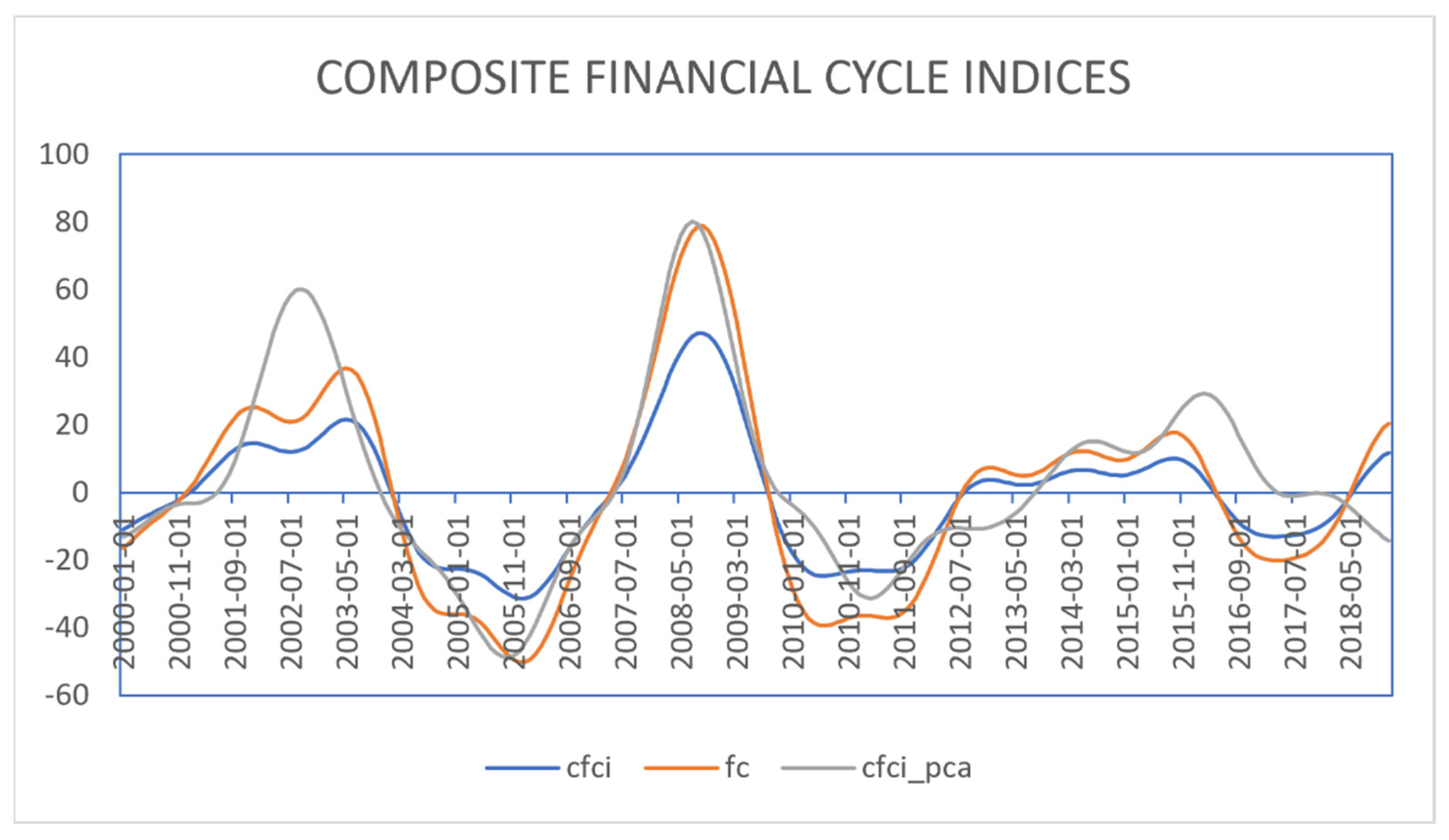
For robustness-checking purposes, the article further constructed two additional financial cycle indices. The first follows the procedure adopted by the SARB to construct a financial cycle index using three variables: credit, house prices, and equity. The second one used 13 financial time series variables and the Principal Component Analysis methodology to construct another robustness-check financial cycle index. All these indices are plotted in Figure A1 in Appendix A. All three indices are shown to follow the same path over time, accurately capturing the main events. What is worth noting is that both the SARB proxy index and the CFCI from PCA appear to be more sensitive to the 2007–2009 global financial crisis. This is shown by the wider swings during this period, while the CFCI swings are relatively moderate, displaying the superiority of the MS-DFM.
For the model, important variables include the output gap, which measures deviations of Real Gross Domestic Product (RGDP) from its potential level. This was achieved by adopting the Christiano–Fitzgerald filter. Short-term interest rates (STIR) show short-term borrowing rates between financial institutions. Inflation (INF) shows changes in the prices of a basket of goods and services. Expected inflation (EINF) represents the survey-based inflation forecasts. Long-term interest rates (LTIR) refer to government bonds maturing in ten years. All these variables were extracted from various sources, including the South African Reserve Bank, the Reserve Bank of St. Louis, and the Bank for International Settlements, among others.
These variables were then tested for stationarity using both the Augmented Dickey–Fuller and Phillips–Perron tests. Once the stationarity properties of these variables were confirmed, various analytical methods were utilised to achieve the set objectives. As an initial step, the article examines the role of financial cycles in business cycle models, specifically analysing whether the financial cycle, as represented by the CFCI, is significant in determining aggregate demand. To achieve this, the article follows in the footsteps of [39] and extends the traditional IS curve equation by incorporating the CFCI variable into the AD function (see Equation (1)). To attain robust results, a Generalised Method of Moments (GMM) is utilised in the regression analysis.
GMM remains predominant in the literature compared to traditional estimation methods such as Ordinary Least Squares (OLS), Two-Stage Ordinary Least Squares (2SLS), and Generalised Least Squares (GLS). Compared with these traditional estimation methods, GMM requires no comprehensive understanding of the underlying data distribution. It can also address endogeneity in explanatory variables, thereby helping to avoid bias due to model misspecification [3]. Although the authors did not conduct tests comparing these methods, we follow the literature’s recommendations in selecting the model adopted in this article.
The GMM estimator, inferred by A which is linear in Y , is given as follows:
β ^ = ( X Z A Z X ) 1 X Z A Z Y
The GMM estimator is said to be consistent, meaning that it converges in probability to β as the sample size approaches infinity [52,53]. However, it is not unbiased, as discussed above. This is mainly because, in finite samples, the instruments are perfectly uncorrelated with the endogenous constituents of the instrumented regressors. We use the above estimator to estimate the reduced form of the hybrid IS curve, which features a link between the financial and business cycles. It imposes the following orthogonality condition:
E t { r G D P t [ μ r G D P t + 1 + α 1 r G D P t 1 + β 1 r r t + β 2 C F C I t ] | v t } = 0
where r r t = ( r t E t π t + 1 ) denotes the real interest rate; v t is a vector of instrument variables at period t ; and it is orthogonal to ε t . The list of selected instruments includes lagged values of all endogenous variables. These instruments are uncorrelated with the disturbance terms and correlated with the explanatory variables.
As a second step, we adopted a Multiple-Equation Generalised Method of Moments (MEGMM) for the regression analysis of the four-equation New Keynesian model. This method allows us to handle a system of multiple equations by specifying the matrices and vectors that comprise a Single-Equation Generalised Method of Moments (SEGMM) [52]. In the presence of heteroscedasticity, the multiple-equation GMM reduces to a Full-Information Instrumental Variable Efficient (FIVE) estimator. It further reduces to a Three-Stage Least Squares model when the set of instrumental variables is common across all equations [52,53,54,55]. Assuming that all regressors are predetermined, the 3SLS diminishes to the Seemingly Unrelated Regressors (SUR) model, which further reduces to the Multivariate Regression (MR) model when all the equations have the same regressors.
An MEGMM can be represented as a system of equations, with coefficients constrained to be equal across equations. Several assumptions are made to derive an MEGMM estimator. These include linearity, ergodic stationarity, orthogonality conditions, and the assumptions that g i is a martingale difference sequence. The definition of the MEGMM estimator is the same as that of the case of an SEGMM, except that the weighing matrix W ^ is now m K m   ×   m K m . Thus, given the above features and assumptions, the multiple-equation GMM estimator is given by:
δ ~ ( W ^ ) = ( S x z W ^ S x z ) 1 S x z W ^ S x y
where S x y is a stacked vector, S x z is a block diagonal matrix, m K m   ×   m K m is the size of the weighting matrix, and g ¯ is the sample mean of g i . The present article utilises this method to obtain unbiased estimates of the four-equation New Keynesian model. Accordingly, assume that v 1 , v 2 , v 3 , and v 4 denotes the instruments for all the four equations in the model, respectively. The set of moment conditions can be illustrated mathematically as follows:
E t { r G D P t [ α 0 + μ r G D P t + 1 + α 1 r G D P t 1 + β 1 r r t + β 2 C F C I t ] | v 1 I N F t [ γ 0 + γ 1 I N F t + 1 + ( 1 γ 1 ) I N F t 1 + γ 2 r G D P t ] | v 2 C F C I t [ [ θ 0 + θ 1 C F C I t 1 + θ 2 r G D P t + θ 3 r t ] | v 3 I N T t [ 0 + 1 I N F t + k + 2 r G D P t + p ] | v 4 } = 0
The chosen instruments are orthogonal to the error terms and differ across equations. Various tests are conducted to validate the model’s output, including the overidentifying restrictions test (J-statistic), the endogeneity test, and the weak-instrument diagnostic test (see Appendix B and Appendix C sections of this article).

2.3. Estimation Results: The Interactions Among BCs, FCs, and MP

The estimation results of Equation one (hybrid IS curve), estimated via the GMM method, are shown in Table 2. Explicitly, we want to ascertain whether the CFCI plays a significant role in determining aggregate demand (AD) in South Africa. We tested the null hypothesis that the CFCI plays no significant role against the alternative hypothesis that it does.
The estimated output in Table 2 above shows that the J-test of overidentifying restrictions yields a p-value of 0.0873. Accordingly, the J-statistic in the model output tests the validity of overidentifying restrictions, which checks whether the instruments are valid, i.e., uncorrelated with the error terms. The null hypothesis is that the instruments are valid, whereas the alternative is that they are invalid. While this value exceeds the conventional 5% rejection threshold, it is nevertheless marginally significant. We therefore interpret this as borderline evidence in favour of instrument validity rather than definitive confirmation.
The test of endogeneity indicated that some of our endogenous variables can be treated as exogenous in the model. Explicitly, the Wu–Hausman tests reported in Appendix B fail to reject the exogeneity null for the financial cycle and interest rate variables in the IS curve (p > 0.10). This finding suggests that, for this specific dataset and instrument set, the endogeneity concerns that typically motivate GMM may be quantitatively mild. However, given the well-established theoretical priors regarding bidirectional feedback between output, interest rates, and financial conditions (e.g., the financial accelerator), and to maintain comparability with the extant literature [3,39], we retain the GMM framework. The Wu–Hausman results are therefore interpreted not as proof of general exogeneity, but as evidence that our chosen instruments adequately satisfy the orthogonality conditions, rendering any finite-sample endogeneity bias empirically negligible. This is a structural property of the South African data during this sample period.
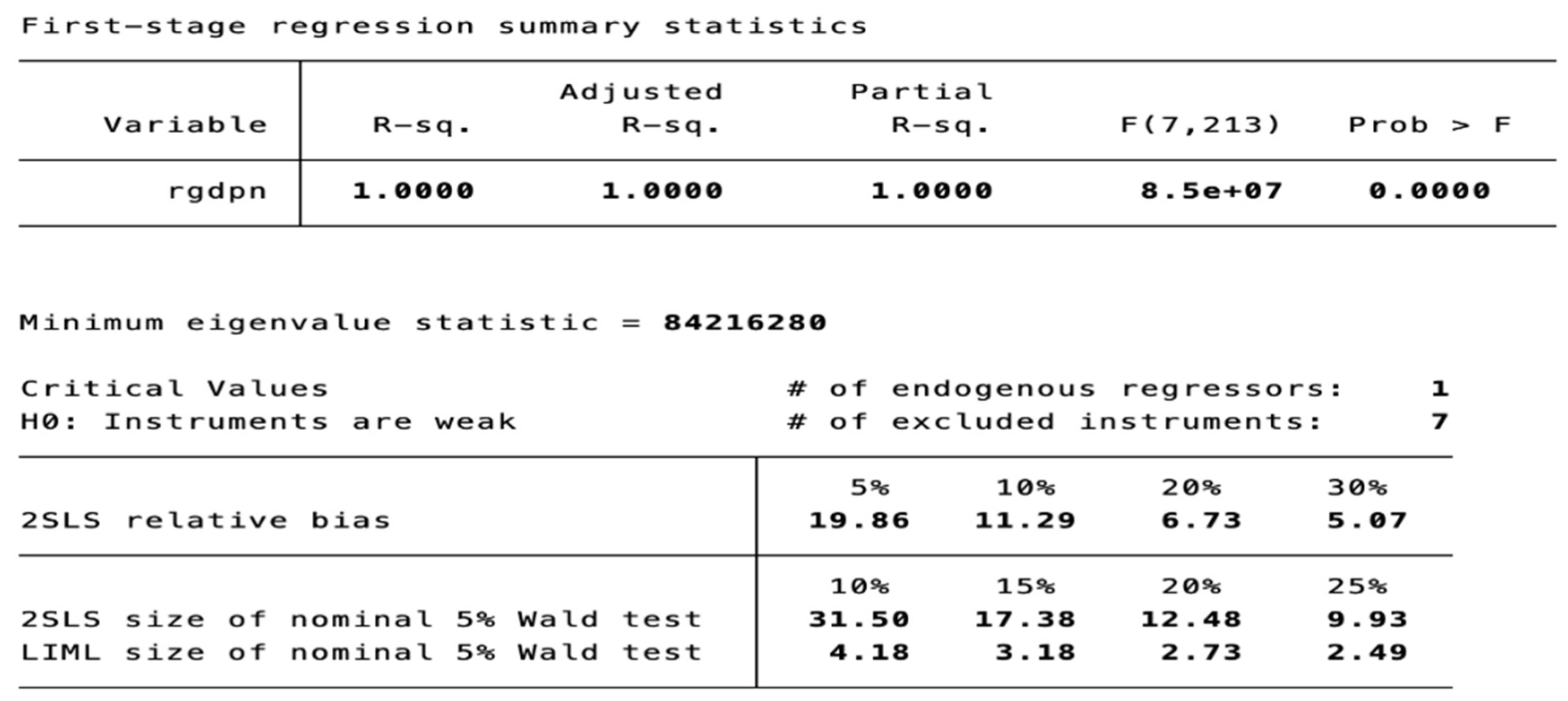
Lastly, the weak-instrument diagnostic tests based on Stock and Yogo’s minimum eigenvalue statistics, the Wald test, and Shea’s adjusted partial R-squared indicated that our instruments are not weak (see Figure A5 in Appendix C). Further, all estimated coefficients attain statistical significance and exhibit the expected signs predicted by macroeconomic theory. Explicitly, the estimates on the coefficients of the backward- and forward-looking elements of the output gap are positive and statistically significant at the 5% level of significance. This indicates that both lag and lead elements of the output gap are important in determining aggregate demand in South Africa.
Further, the coefficient on the rate of interest (real) is, as expected, negative and significant at the 5% significance level. This is also in line with macroeconomic theory, which predicts that an increase in the real rate of interest will lead to a deterioration in investment, thus decreasing aggregate demand and the output gap. Furthermore, in line with the aforementioned rule regarding the IS puzzle, the article finds a significant negative effect of the interest rate on output and therefore concludes that there is no evidence of the IS puzzle in South Africa during the period under examination.
Importantly, the relationship between the output gap and CFCI is such that a one-unit increase in CFCI leads to a 0.007 percentage point increase in the output gap. This value is positive and significant at the 5% level, indicating a positive relationship between the output gap and the CFCI. Therefore, the null hypothesis that the CFCI plays no role in determining AD in South Africa is rejected at the conventional 5% significance level. It is concluded that the CFCI plays a significant role in determining AD in South Africa. This indicates that incorporating the CFCI into business cycle models is vital to modern economics and subsequent policy analyses. Therefore, to stabilise output in South Africa, the SARB needs to consider developments and the effects of the CFCI in accordance with the procyclicality theory of the relationship between financial stability and the real economy. For robustness-checking purposes, the same IS curve was estimated, this time including the SARB proxy financial cycle index. The results, shown in Table A2 in Appendix A, are consistent with the conclusions drawn above.
Consistent with the second objective of this article, the estimation results for the four-equation New Keynesian framework, obtained using a multiple-equation GMM approach, are shown in Table 3. Specifically, it is asked whether there exists a unified macroeconomic framework in South Africa that links the macroeconomy and the financial system. Harmonised with the literature [3,56,57], all dependent variables are treated as endogenous, while lagged endogenous variables are treated as exogenous. First, the test of overidentifying restrictions is examined, as shown in Table 3.
In the simultaneous model, the overidentifying restrictions test tests two different things simultaneously. As a rule of thumb, a significant test statistic could represent either invalid instruments or incorrectly specified structural equations. For the model, the J-test of overidentifying restrictions yields a p-value of 0.0665. While this value exceeds the conventional 5% rejection threshold, it is again marginally significant. This will therefore again be interpreted as borderline evidence in favour of instrument validity rather than definitive confirmation. In policy-oriented DSGE modelling, such marginal p-values warrant caution and motivate the subsequent sensitivity analysis conducted in Section 3.7.
We further tested for exogeneity in our endogenous variables on an equation-by-equation basis. The results indicated that some of our endogenous variables can be treated as exogenous in the model. Specifically, the Wu–Hausman tests presented in Appendix B do not reject the null hypothesis of exogeneity for the financial cycle and interest rate variables in the IS curve (p > 0.10), nor for the output gap in the Phillips Curve. This indicates that, within this dataset and instrument specification, the endogeneity issues that typically justify the use of GMM appear to be relatively limited in magnitude. Nonetheless, given the strong theoretical expectations of bidirectional relationships among output, interest rates, and financial conditions, such as those described by the financial accelerator, and to ensure consistency with existing literature [3,39], the Multiple GMM approach is retained. The Wu–Hausman results are therefore not interpreted as confirming general exogeneity, but rather as suggesting that the selected instruments satisfy the orthogonality conditions effectively, making any finite-sample endogeneity bias empirically insignificant. This outcome reflects a structural characteristic of the South African data during the period under study (see Table A6, Table A7, Table A8 and Table A9 in Appendix B).
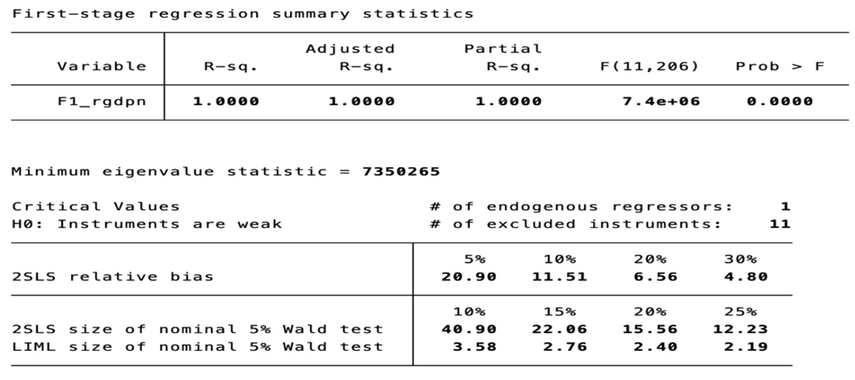
Lastly, we conducted a weak-instrument equation-by-equation analysis. Using the Craigg–Donald F-test, Shea’s adjusted R-squared, the Wald test and Stock and Yogo’s minimum eigenvalue statistics, it was confirmed across all equations that our instruments are not weak (see Figure A5, Figure A6, Figure A7 and Figure A8 in Appendix C).
Looking at the jointly estimated output of the model presented in the table, and following the scrutiny in the preceding subsection, the hybrid IS curve in the model system shows that all calculated coefficients have the anticipated signs and are statistically significant, consistent with economic theory. Notably, there is no significant difference in the coefficient estimates from the joint model and the single-equation estimation presented above. The interpretation of these results, therefore, remains the same as above.
The estimation results for the Phillips Curve indicate that all estimated coefficients have the anticipated signs and are statistically significant. Overtly, the estimation results indicate that both lagged and expected inflation rates have a positive and statistically significant effect on the current level of inflation, with lead inflation exerting a larger effect than lag inflation. Further, the output gap factor is shown to be positive and highly statistically significant, consistent with prior and theoretical expectations.
A major novelty of this article is the inclusion of the equation that captures the evolution of the financial cycle in the New Keynesian model. The estimation results for this equation are consistent with the stylised features of financial cycles found in the literature [58]. Specifically, the coefficients on the lagged CFCI and the output gap are statistically significant at all levels and are positive. This shows substantial persistence and co-movement between the CFCI and the business cycle. The coefficient on the nominal interest rate is statistically significant at all levels of significance and is negative. This shows an inverse association between interest rates and CFCI, as theory predicts that interest rates are correlated with a downward phase of the financial cycle.
Lastly, the estimation of the forward-looking monetary policy rule indicates that we attain the desired results, with estimated coefficients that are statistically significant and have the anticipated signs over the full sample period. These results indicate that the SARB has been aggressive towards interest rate smoothing and output gap stabilisation rather than inflation, consistent with Taylor’s principle. However, the SARB has also been more focused on the output gap than on anticipated inflation, even though sluggishly, which helps confirm the SARB’s mandate of price stability. These results also suggest a strong preference for gradualism in the SARB’s interest rate setting. For robustness-checking purposes, we re-estimated the four-equation model using a different specification of the financial cycle, namely the SARB proxy index. The results, shown in Table A3 in Appendix A, are within the theoretical expectations; however, they show relative sensitivity to different specifications of the CFCI.
Overall, while the estimated results above provide insights into the nature and importance of the relationships among business cycles, financial cycles, and monetary policy in South Africa, we cannot generalise their applicability beyond the sample period. Accordingly, it is rather naïve to predict the effects of economic policy changes based on semi-structural relationships derived mainly from highly aggregated historical data (Lucas Critique). The models estimated above are not built on micro foundations. This indicates that the model parameters are not structural and therefore may not be policy-variant. As a result, they may not change whenever there is a policy change. To understand how the collective decisions of rational individuals, coordinated across a range of variables, relate to both present and future outcomes, as well as the wider effects of the financial–real trade-off and the dynamic effects of policy responses by the monetary authorities, a Dynamic Stochastic General Equilibrium model calibrated using South African data is formulated.

3. General Equilibrium Framework

3.1. Model Overview

We develop a small open-economy New Keynesian Dynamic Stochastic General Equilibrium (DSGE) model that captures the interactions among business cycles, financial cycles, and monetary policy in South Africa. The model is designed to study monetary policy responses to macroeconomic and financial disturbances in South Africa. The model amalgamates a forward-looking IS relationship, a forward-looking New Keynesian Phillips curve, a persistence-driven financial cycle, a standard Taylor-type monetary policy rule, and a small open-economy foreign sector. Investment and capital accumulation are represented in a simple linearised form. Shocks to demand, inflation, the policy rate, the composite financial cycle index, technology, foreign output, foreign inflation and investment drive the dynamic interactions [59].
The model aggregates the economy into six sectors: households, final goods firms, the financial sector, the monetary authority, capital accumulation, and the foreign sector. The representative household supplies differentiated labour and chooses consumption and investment, subject to standard intertemporal trade-offs, which are represented here by a reduced-form IS curve and an investment rule. Final goods firms produce output under monopolistic competition and Calvo price-setting frictions. The New Keynesian Phillips curve (NKPC) arises from price adjustment costs and mark-up behaviour, and marginal cost maps into inflation dynamics. The financial sector is captured by an aggregate financial cycle variable, C F C I , with persistence and an influence on both demand and monetary conditions. The variable stands in for broadly defined financial amplification and enters the IS curve and the financial cycle equation as a persistent, partially inertial process [59,60] (Steinbach, Mathuloe et al. 2009, Gupta, Hollander et al. 2020).
The monetary authority sets the nominal policy rate according to a forward-looking Taylor-type rule that responds to inflation and the output gap and may include smoothing. The central bank is modelled as a reduced-form policymaker that may or may not respond directly to the financial cycle. Capital accumulates via a standard law of motion with depreciation. Investment is expressed in a linearised reduced form that links investment to the output gap and an investment shock. Finally, the foreign sector is captured by exogenous autoregressive processes for foreign output and foreign inflation, both of which are persistent. These capture external demand and price pressures that feed into the domestic economy through the open-economy channel. The model equations are provided below.

3.2. Model Setup Equations (Level Form)

The present section provides a set of micro-founded Dynamic Stochastic General Equilibrium (DSGE) equations together with the first-order, or optimality, conditions for all agents. These agents include households, firms, capital/investment, the monetary policy, and the financial sector. The equations are given in both level form and log-linearised form [61,62].

3.2.1. Households

We assume a representative household that maximises lifetime utility according to the following utility function:
E 0 t = 0 β t [ U ( C t b C t 1 , N t ) ]
with period utility given as:
U ( C t b C t 1 , N t ) = ( C t b C t 1 ) 1 σ 1 1 σ χ N t 1 + φ 1 + φ
where b is the external habit formation variable, σ captures the inverse intertemporal elasticity, φ is the inverse Frisch elasticity, and χ is the weight of labour disutility. The subject budget constraint faced by the representative household is given as follows:
P t C t + P t I t + B t + 1 = W t N t + ( 1 δ ) P t K t + R t 1 B t + Π t
where B t captures nominal bond holding, R t 1 captures the gross nominal rate of return, Π t measures firms’ profit, I t denotes investment, and K t is capital accumulation. We assume that capital accumulates in accordance with the usual law of motion of capital, given as follows:
K t + 1 = ( 1 δ ) K t + I t

3.2.2. Firms or Production

We assume that aggregate final goods are produced under monopolistic competition by a continuum of firms i , with Calvo pricing. Accordingly, a typical firm faces demand given as follows:
Y i , t = ( P i , t P t ) ε Y t
Production follows the usual Cobb–Douglas production function, with technology showing total factor productivity (TFP), as follows:
Y i , t = A t K i , t α L i , t 1 α
where A t is a technological factor that captures total factor productivity, while α and 1 α measure the contributions of capital and labour to total production, respectively. Real marginal cost m c t is derived from cost minimisation.

3.2.3. Financial Cycle (Reduced Form)

The equation that captures developments in the South African financial system is given as follows:
C F C I t = ρ F C F C I t 1 + α y y t + α r r t + ε t C F C I
with ρ F capturing the persistent nature of the financial system, α y capturing the procyclical nature of the financial system and the real economy, and α r capturing the relationship between the financial cycle and the real interest rate. Accordingly, the real interest rate is negatively associated with the financial cycle, as it typically coincides with its downturn. The financial cycle equation (Equation (20)) is specified in reduced form rather than derived from micro foundations, consistent with the approach adopted by [58,59]. This pragmatic choice reflects the complexity of modelling South Africa’s financial system structurally and is acknowledged as a limitation. The equation captures three well-established empirical regularities, viz., persistence, procyclicality, and the countercyclical effect of interest rates, without imposing a specific financial friction mechanism.

3.2.4. Monetary Authority

It is assumed that the monetary authority follows a Taylor rule-type monetary policy. The nominal interest rate rule is given as follows:
i t = ρ i i t 1 + ( 1 ρ t ) ( ϕ π π t + ϕ y y t + ϕ C F C I C F C I t ) + ε t m
The central bank sets the nominal interest rate with an interest rate smoothing parameter of ρ i , while also responding to inflation and the stability of the output gap. ϕ C F C I captures the response of monetary policy to financial stability. In the baseline model, ϕ C F C I = 0 , showing no response to financial stability, while in the alternative or augmented case, ϕ C F C I > 0 , showing a monetary policy response to financial stability.

3.3. First-Order/Optimality Conditions

The present section provides the first-order conditions and optimality conditions derived from the level equations above. These include the Euler equation, the labour supply function, and the firm’s pricing first-order conditions. Also included are the investment and capital optimality conditions [62].

3.3.1. Household FOCs

Let c t = C t b C t 1 . The household FOCs are as follows:
Intertemporal Euler (Nominal/Real)
The real Euler equation for the real bonds is as follows:
1 = E t [ β U c ( c t + 1 , N t + 1 ) U c ( c t , N t ) R t + 1 r ]
where U c = U c . Using R t + 1 r 1 + i t 1 + π t + 1
Intertemporal Labour Supply
The intertemporal labour supply equation is derived as follows:
U n ( c t , N t ) + U c ( c t , N t ) . W t P t = 0

3.3.2. Firm Prising/Calvo Pricing and NKPC

With Calvo pricing, a profit-maximising firm will choose a price P t * and maximise expected discount profit as follows [61]:
m a x P t * E t k = 0 θ k Q t , t + k ( P t * Y t + k | t P t + k M C t + k Y t + k | t )
where Q t , t + k is a stochastic discount factor, and Y t + k | t is the demand for the price set at period t in period t + 1 . The log-linearised forward-looking New Keynesian Phillips curve equation is then given as follows:
π t =   β E t [ π t + 1 ] + ( 1 θ p ) ( 1 β θ p ) θ p m c t + e t π
where inflation is assumed to depend on expected future inflation (the forward-looking term from Calvo pricing) and real marginal cost, m c , with a slope determined by price stickiness θ p and the elasticity of substitution in goods ε p . e π is an inflation shock (Tovar, 2008) [61].

3.3.3. Market-Clearing Condition

The real aggregate resource constraint is as follows:
Y t = C t + I t + G t + ( N X ) t + ε t y
where Y t   is the aggregate output gap, C t is the aggregate consumption expenditure, I t is the aggregate investment expenditure, G t is the aggregate government expenditure and ( N X ) t denotes the difference between exports and imports, known as net exports.

3.3.4. Financial Cycle Equation

The basic structure of the financial system follows Equation (20) from above. The interpretation of the components remains the same; hence, we will not repeat the equation and its interpretation here.

3.4. Log-Linearised Equilibrium System

The basic structure of the model follows that of [59,60]. It is a two-country New Keynesian open-economy framework, with the foreign country as the rest of the world and the domestic country as South Africa, which is assumed to be a small open economy. The model assumes a staggered price- and wage-setting mechanism analogous to that used by [63]. Each equation used in the model implementation is shown below. The variables used are expressed log deviations from the steady state unless otherwise stated. The semi-structural rule in Equation (4) is forward-looking and serves the GMM estimation in Section 2. The DSGE rule in Equation (21) is backward-looking in the smoothing term, which is the standard formulation for Dynare implementation. The two are not identical by design; the DSGE version embeds the financial cycle term ϕ C F C I , which is absent from the reduced-form GMM, consistent with the policy experiment described in Section 3.6.
y g a p t = h y g a p t + 1 1 σ ( r t π t ) + κ c f c i c f c i t + e t y ( IS   curve ( Forward - looking ) )
π t = β E t [ π t + 1 ] + κ m c t + e t π ( New   Keynesian   Phillips   curve ( forward - looking ) )
c f c i t = ρ c f c i c f c i t 1 + κ c f c i y g a p t + θ c f c i ( r t π t ) + e t c f c i ( Financial   system )
r t = ρ r r t 1 + ( 1 ρ r ) ( ρ π π t + ρ y y g a p t + ρ c f c i c f c i t ) + e t r ( Monetary   policy )
m c t = σ 1 h ( y g a p t h y g a p t 1 ) + ϕ y g a p t ( 1 ϕ ) z t ( Real   marginal   cost )
z t = ρ z z t 1 + e t z ( Technology ( AR ( 1 ) ) )
y t f = ρ f y t 1 f + ε t f ( Foreign   sector   output )
π t f = ρ π f π t 1 f + ε t π f ( Foreign   sector   inflation )
k t + 1 = ( 1 δ ) k t + δ i t ( Capital   accumulation )
i t = ρ t i   i t 1 + γ y y t + e t i ( Investment )

3.5. Calibrations

The calibrated parameters of our model are borrowed from various sources in the literature, including [23,64,65,66,67,68].
Many of them are consistent with the findings of [69,70]. Table 4 presents a summary of the parameters, their descriptions and their respective sources. The discount rate indicates how consumers value present versus future consumption. The Calvo price stickiness value of 0.75 suggests that there is a 25% probability that firms will change their prices in each period. This is relevant to South Africa and is widely applicable in the South African Reserve Bank (SARB) studies. It acknowledges that not all firms will change their prices simultaneously, thereby accounting for possible price stickiness. The steady state inflation rate is 0.005, which is a midpoint well within the 3–6% range, as per the SARB mandate. Also worth mentioning is that the composite financial cycle amplification and persistence coefficients are 1.092 and 0.924, respectively. These values are extracted from the developed CFCI and are in accordance with the South African credit cycle estimates [23,24,68,71].

3.6. Simulation Results and Inferences

This section presents the simulated dynamics and impulse response analysis derived from the calibrated DSGE model. The purpose of the simulations is to examine how the South African economy responds to various structural shocks under a monetary policy framework that interacts with the financial cycle. Using the calibrations described in the previous section, the model is solved using a first-order perturbation method in Dynare, and impulse response functions (IRFs) are generated for key macroeconomic and financial variables, namely, the output gap, inflation, the policy interest rate, the financial cycle index, investment, and capital. These simulations allow us to trace the propagation mechanisms of real, nominal, and financial disturbances, as well as to assess the stabilising role of monetary policy. We begin by examining the variance decompositions of our key variables under both the base Taylor and the augmented Taylor rules.
According to Table 5, most of the variation in the output gap originates from shocks to the output gap itself, although shocks to the financial cycle and technology also play a role. At the same time, most of the variation in the financial cycle is seen to originate from technological shocks and shocks to the financial system itself. Most of the variation in capital originates from an investment shock. In contrast, most of the variation in investment originates from shocks to itself and to the output gap. The remaining variables are shown to fluctuate primarily due to technological shocks.
The results in Table 6 are not very different from those in Table 5. Most importantly, with regard to the interactions among the financial system, the real economy, and monetary policy, once the SARB begins responding to financial system dynamics, less variation in the output gap is driven by the financial system. This is proof that treating financial stability as a secondary objective of monetary policy can be rather stabilising for both the financial system and the real economy. This is also supported by the reduced variation in the financial cycle following a shock to the output gap. Again, the effect of a financial cycle shock on inflation and the interest rate remains relatively mild under both regimes, which also validates the adoption of financial stability within the functioning of the SARB.
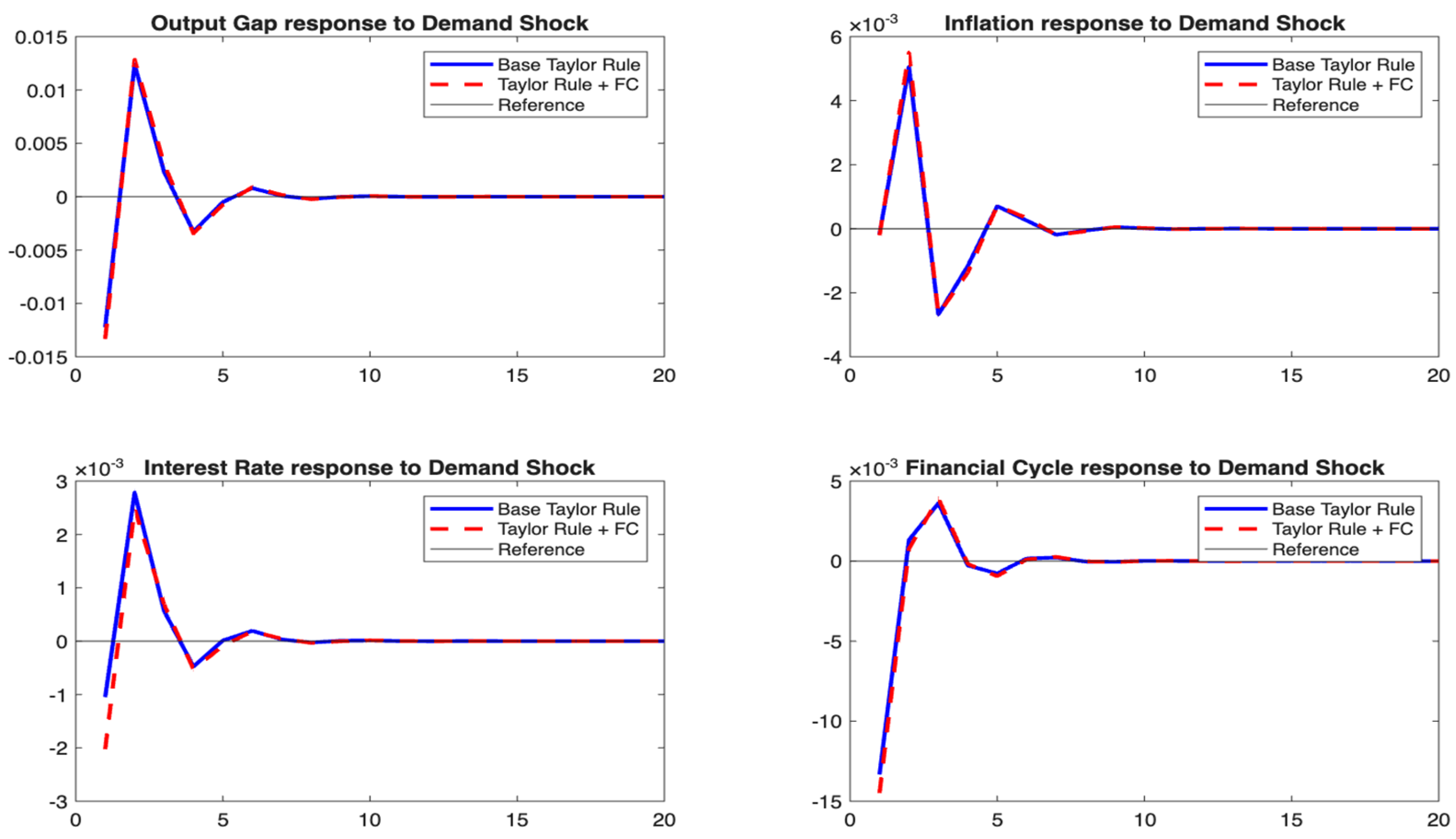
We further provide the impulse response functions following the variance decomposition analysis. As previously done, we compare alternative policy regimes: one in which the central bank responds only to inflation and output, and another that explicitly includes financial system considerations. The results should provide insights into the strength of financial–real linkages in South Africa and the policy trade-offs faced by the SARB in balancing price and financial stability objectives. Figure 2 below summarises the impulse response functions of all endogenous variables of the model in response to a positive demand shock.
Under both policy regimes, a positive demand shock temporarily increases output, inflation, interest rates, and the financial cycle, with all variables returning to equilibrium after about seven quarters. Crucially, adding a financial stability target to the central bank’s mandate (moving from responding only to inflation and output) does not cause significant deviations in outcomes. Instead, the dotted red line consistently lies below the blue line across all graphs, indicating that incorporating financial stability improves the stabilisation of both the real economy and the financial system.
Figure 2. Response of endogenous variables to a positive demand shock. Source: Authors’ depiction.
Forecasting 08 00051 g002
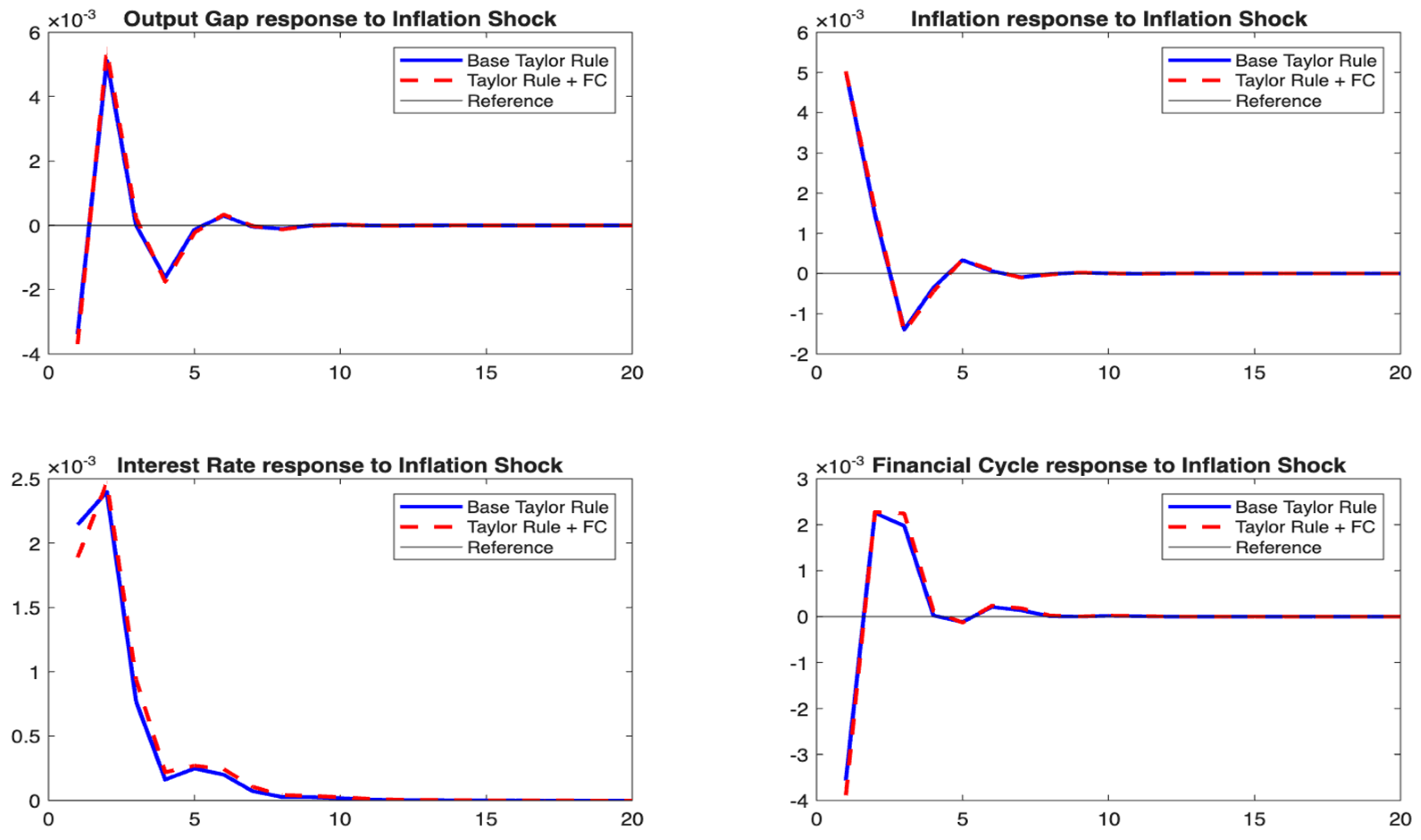
A positive inflation shock initially contracts output, which then rebounds and stabilises after about 10 quarters (see Figure 3). Adding a financial cycle term to the Taylor rule slightly dampens volatility in the output gap. Inflation rises immediately but returns to the steady state as interest rates rise, with nearly identical disinflation paths under both rules, showing that inflation targeting remains robust. The policy rate rises sharply, peaking within the first quarter. Under the financial-augmented rule, the rate increase is slightly more front-loaded, although inflation remains the main driver. The financial cycle initially moves upward and oscillates mildly; these oscillations are more muted under the augmented rule, indicating that leaning against the financial cycle smooths credit and asset dynamics without disrupting the real economy.
Figure 3. Response of endogenous variables to a positive inflation shock. Source: Authors’ depiction.
Forecasting 08 00051 g003
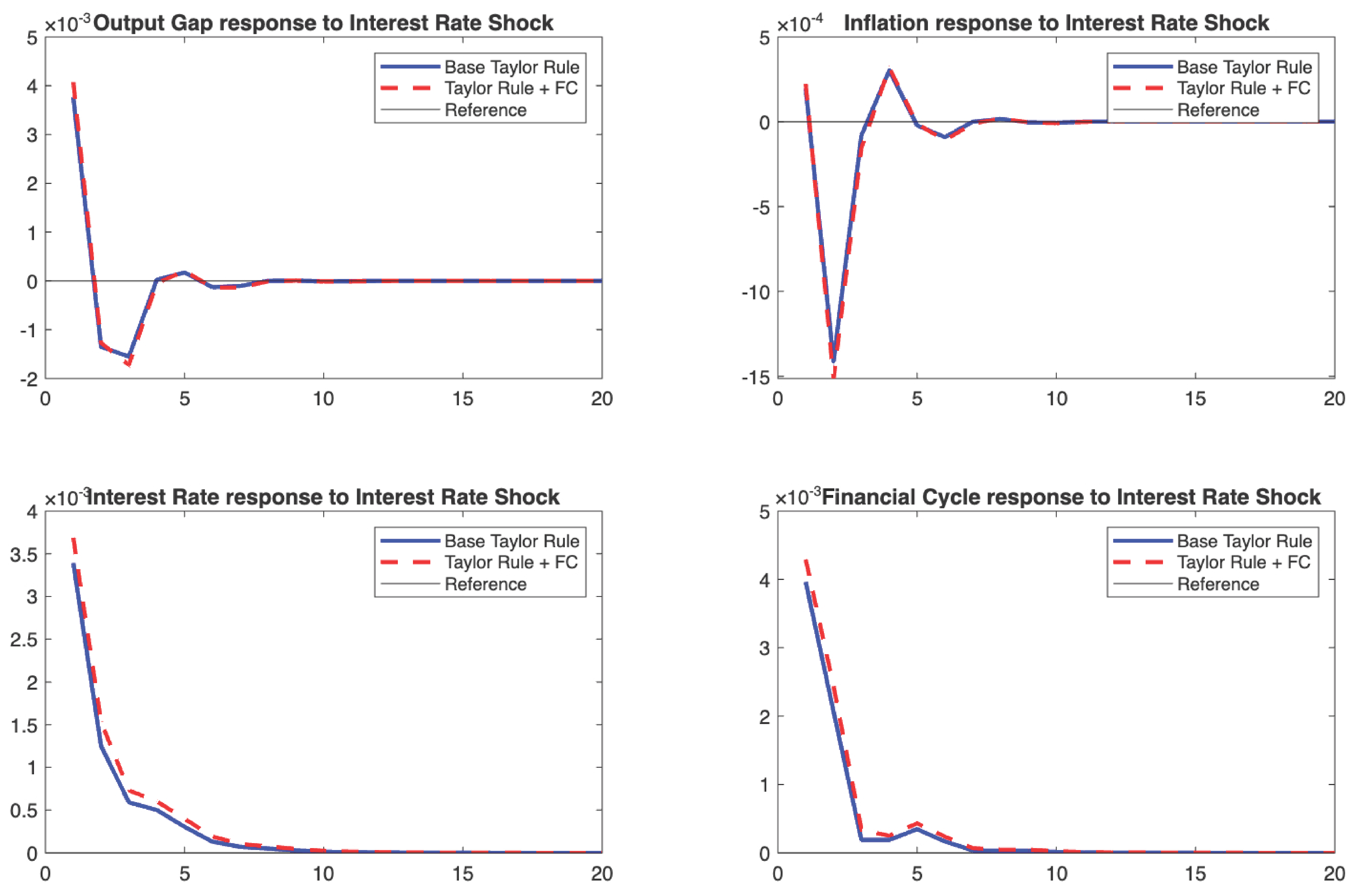
Inflation falls sharply after the interest rate hike, briefly rebounds, and then stabilises (see Figure 4). Both policy rules yield nearly identical inflation responses, showing that adding the financial cycle does not harm inflation stabilisation or the credibility of inflation targeting. The policy rate rises sharply on impact and decays gradually. Under the augmented rule, the adjustment is slightly more persistent, suggesting a stronger and more sustained policy response when financial stability is monitored. The financial cycle declines immediately after the tightening shock and then rebounds mildly. Under the augmented rule, this reaction is less volatile, confirming that responding to financial conditions helps mitigate procyclical financial swings and reduces the propagation of systemic risk.
Figure 4. Response of endogenous variables to a positive interest rate shock. Source: Authors’ depiction.
Forecasting 08 00051 g004
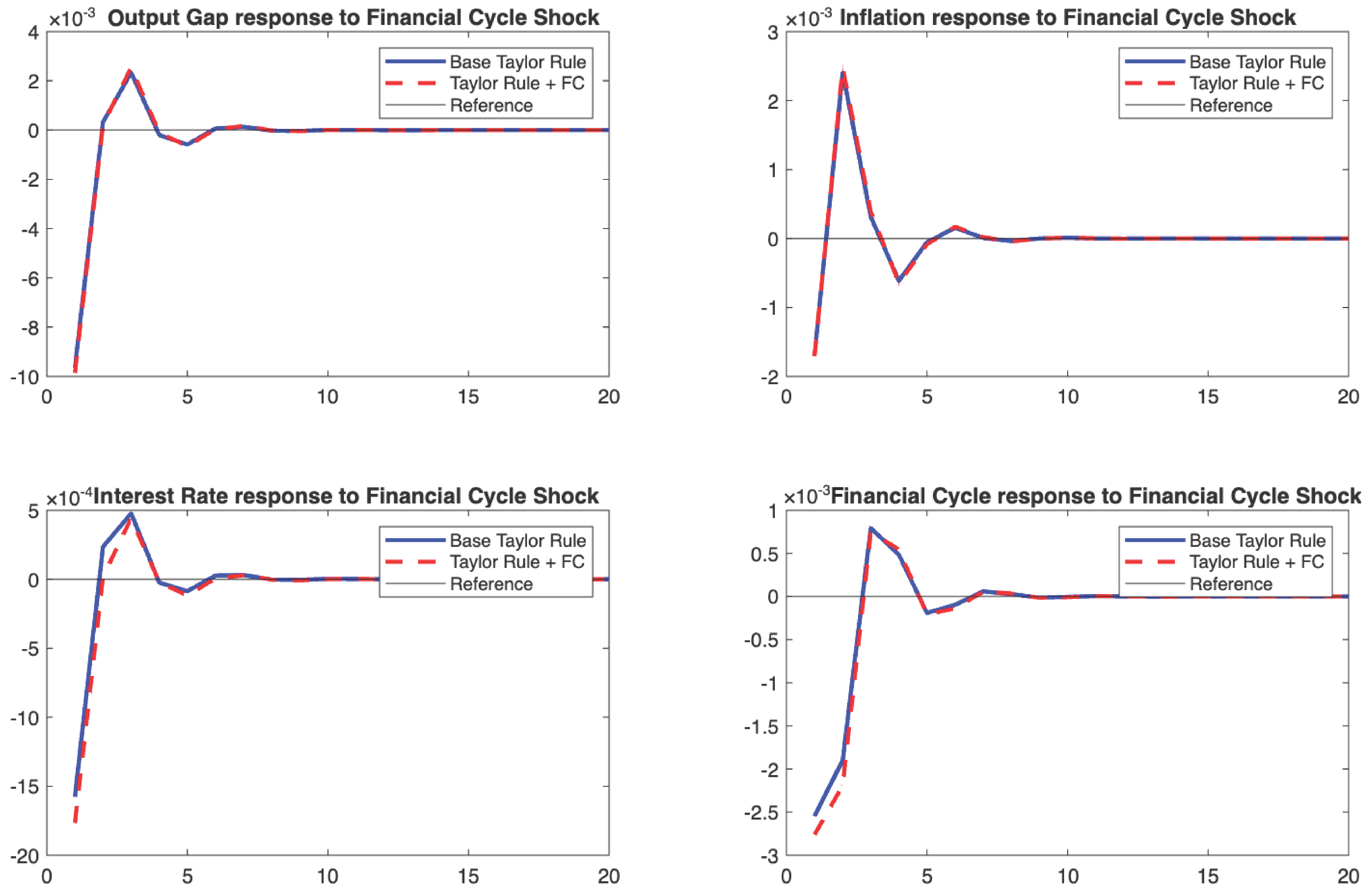
Lastly, a positive financial cycle shock (e.g., an upturn in credit or asset markets) initially reduces the output gap, followed by a short-lived rebound and a gradual return to equilibrium (see Figure 5). When the financial cycle is included in the monetary rule (red dashed line), the initial output contraction is slightly smaller, indicating that policy that responds to financial conditions helps cushion the real economy against such shocks.
Inflation initially declines and then briefly rises, with nearly identical paths under both policy regimes. This shows that financial shocks have limited short-run price effects and that incorporating financial stability does not distort inflation control, preserving the inflation-targeting mandate. The policy rate rises immediately in response to the financial shock, peaks, and then decays quickly. Under the augmented rule, the interest rate adjustment is slightly more aggressive and persistent, signalling that the central bank leans more strongly against excessive financial expansion, thereby enhancing systemic resilience and moderating risk-taking incentives.
Explicitly, the financial cycle itself rises sharply in the first period following the shock, consistent with the model’s design, reflecting a burst of credit growth or asset appreciation before reverting to the steady state. With the augmented Taylor rule, the amplitude of the financial cycle is marginally dampened, confirming that integrating financial stability into monetary policy can reduce the persistence of financial booms and soften the amplitude of the credit cycle. This demonstrates that a policy rate that reacts to financial indicators can “lean against the wind”, helping to contain macro-financial feedback loops.

3.7. Sensitivity Analysis

For the sensitivity analysis, we re-estimated the model for lower values of the coefficient κ _ c f c i   = 0.1 and a higher value of the coefficient κ _ c f c i   =   1.6 , compared to the base of the coefficient κ c f c i = 1.092 (see Table A4 and Table A5). The sensitivity analysis varies the policy coefficient in the Taylor rule (from a baseline value of 0.1 to 1.6) to assess robustness. Under the baseline, variance is largely explained by a few dominant shocks, with some variables showing persistence over 90%. With a low coefficient (0.1), variance becomes highly concentrated in a few shocks, with extreme dependence on single disturbance sources (70–90%+), indicating weakened shock distribution across channels.
With a high coefficient (1.6), variance becomes more evenly distributed, leading to broader shock transmission and greater interaction among variables, reflecting stronger propagation and more balanced responses. The model is structurally robust, but the distribution and dominance of shocks are highly sensitive to the policy coefficient. Low coefficients cause concentration and instability, whereas higher coefficients promote dispersion and resilience. Proper calibration of monetary policy rules is critical for effective shock absorption and macroeconomic stability.

3.8. Discussion of Findings

The results show that the financial cycle is a key driver of aggregate demand in South Africa, meaning that monetary policy must account for both output dynamics (past and expected) and financial conditions to stabilise the economy effectively. Ignoring financial factors can lead to mismeasurement of aggregate demand, instability in the output gap, and potential recessions. Additionally, the findings provide empirical evidence that the IS puzzle is not present in South Africa, reinforcing the relevance of financial variables in business cycle analysis.
Secondly, the results indicate that the composite financial cycle index (CFCI) in South Africa is highly persistent, aligning with the stylised fact that financial cycles are longer and more pronounced than business cycles. This finding is supported by both local studies [e.g., [71,75]] and the international literature [51,76,77,78], all of which confirm that financial cycles exhibit greater duration and amplitude compared to conventional business cycles.
Further, these results provide evidence of the financial system’s procyclicality. One interpretation of these results is that the South African CFCI exhibits substantial co-movement with the South African business cycle. The stylised features of financial cycles and empirical evidence on the correlation between business and financial cycles largely support this finding. For example, in [79,80], it was shown that robust connections exist between the different phases of business and financial cycles. These results also suggest the existence of a mutually reinforcing mechanism through which the financial system can intensify macroeconomic oscillations, potentially leading to or exacerbating financial imbalances. Hence, it can be posited that the SARB needs to consider developments in the output gap when seeking to stabilise the financial system [see also [68]]. These findings are in line with the analysis of the IS curve discussed above.
Furthermore, the model system results demonstrate the existence of a unified macroeconomic framework in South Africa that features both a financial system target and a real system target. This is evident in the finding that the inclusion of a financial system equation within the model does not destabilise the system; rather, it complements it and improves its stability. This is proof that a macroprudential or financial stability mandate can be incorporated into the functioning of the South African Reserve Bank. Nevertheless, a responsibility for such a mandate should reside with a separate committee in addition to the Monetary Policy Committee. These results align with analyses in the previous literature [see [23]].
The impulse response analysis shows that monetary and financial shocks are transmitted through interconnected real, nominal, and financial channels and that the model exhibits stable, mean-reverting dynamics under a credible inflation-targeting framework. The baseline Taylor rule effectively stabilises inflation and output. When the financial cycle (CFCI) is included in the policy rule, outcomes improve, output and financial volatility are reduced, and financial shocks become less persistent and less pronounced, without compromising inflation performance. The augmented rule also leads to a more proactive and sustained policy response, helping to curb financial excesses during booms and support smoother adjustments during downturns. Overall, incorporating financial conditions enables monetary policy to better balance price stability and financial stability, effectively “leaning against the wind” of financial imbalances.

4. Summary and Conclusions

The article’s overall findings clearly show significant interactions between the real and financial economies in South Africa. Further, financial factors and financial shocks play a significant role in BC fluctuations. Hence, we posit that, given the configuration of BC models in South Africa, monetary authorities need to consider the distinct and significant effects of these financial factors to achieve a true reorientation of the BC. Further, to stabilise both the real economy and the financial system, the SARB needs to consider development in both streams, as they are highly interrelated. Furthermore, the evidence suggests that the SARB’s decisions aimed at promoting price stability should be informed, in part, by developments in the financial system. This clearly shows that failure to include financial factors and consider financial shocks might complicate policy initiatives, increase the risk of crises, and question the credibility of the central bank.
Moreover, the findings highlight that, for an emerging market like South Africa, characterised by deep financial linkages and sensitivity to global liquidity conditions, integrating financial cycle indicators into the monetary policy framework strengthens macroeconomic resilience. Such an approach enables the South African Reserve Bank (SARB) to better manage the trade-offs among price stability, output stabilisation, and financial stability, thereby reinforcing the case for a more inclusive and forward-looking monetary policy strategy.
The simulation results underscore the importance of incorporating financial stability considerations into South Africa’s monetary policy framework. While the traditional Taylor rule remains effective in anchoring inflation expectations, it is less equipped to address fluctuations arising from financial imbalances. By contrast, a financially augmented Taylor rule enables the South African Reserve Bank (SARB) to respond more systematically to credit, leverage, and asset price dynamics, thereby reducing the likelihood of procyclical financial amplification. Such an approach would allow the SARB to act pre-emptively during periods of financial exuberance and provide measured support during downturns, ultimately promoting a more stable and inclusive macroeconomic environment without compromising the inflation-targeting mandate.
It is worth noting that the current study relies on calibrated parameters, which may, at times, pose challenges for making informed policy decisions. Other methods, such as Bayesian DSGE models, could be applied in future studies to address this limitation.

Author Contributions

Conceptualisation, M.C.N., C.T. and P.-F.M.; methodology, M.C.N.; software, M.C.N.; validation, M.C.N., C.T. and P.-F.M.; formal analysis, M.C.N.; investigation, M.C.N.; resources, M.C.N.; data curation, M.C.N.; writing—original draft preparation, M.C.N.; writing—review and editing, M.C.N. and P.-F.M.; visualisation, M.C.N.; supervision, C.T. and P.-F.M.; project administration, M.C.N.; funding acquisition, M.C.N. All authors have read and agreed to the published version of the manuscript.

Funding

This research received no external funding.

Data Availability Statement

The data used in this study were obtained from various public sources, including the South African Reserve Bank Database, the Federal Reserve Bank of St. Louis, the Bank for International Settlements, and the Organisation for Economic Co-operation and Development.

Conflicts of Interest

The authors declare no conflicts of interest.

Abbreviations

The following abbreviations are used in this manuscript:
BCBusiness Cycle
FCFinancial Cycle
CFCIComposite Financial Cycle Index
DSGEDynamic Stochastic General Equilibrium
GMMGeneralised Method of Moments
MEGMMMultiple-Equation GMM
NKPCNew Keynesian Phillips curve
SARBSouth African Reserve Bank
GFCGlobal Financial Crisis
IRFImpulse Response Function
VDVariance Decomposition

Appendix A

Figure A1. Composite financial cycle indices.
Forecasting 08 00051 g0a1
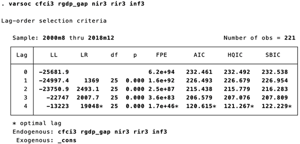
Table A1. Number of lags used in GMM and MEGMM estimations.
NO OF LAGS USED PER EQUATION (VARSOC—INFORMATION CRITERION)
IS CURVEUSED LAGS 1-4 OF:
OUTPUT GAP,
INTEREST RATE
AND THE FINANCIAL CYCLE
PHILLIPS CURVEUSED LAGS 1-4 OF:
OUTPUT GAP,
AND INFLATION
FINANCIAL CYCLEUSED LAGS 1-4 OF:
FINANCIAL CYCLE,
OUTPUT GAP,
AND INTEREST RATE
TAYLOR RULEUSED LAGS 1-4 OF:
NOMINAL INTEREST RATE
OUTPUT GAP,
INFLATION,
AND THE FINANCIAL CYCLE
Forecasting 08 00051 i001
Table A2. IS curve with SARB proxy index.
Dependent Variabley
y t + 1 0.468 ***
(0.003)
y t 1 0.543 ***
(0.004)
r i r t + 1 −0.086 ***
(0.000)
c f c i 0.007 ***
(0.000)
J-statistic (p-value) 66.6811
(0.0699)
Note: Significance at the 1% levels is reported by ***. Standard errors are in parentheses. Source: Authors’ estimates (2026).
Table A3. Four-equation model with SARB proxy index.
EquationParameterDescriptionValueJ-Statistic
(p-Value)
Extended IS curve y t = μ E t y t + 1 + α 1 y t 1 + β 1 ( r t E t π t + 1 ) + β 2 F C t + ε t y 87.4416 (0.0975)
μ Lead of the output gap0.335 *** (0.003)
α 1 Lag of the output gap1.014 *** (0.010)
β 1 Lead of the real interest rate gap−0.002 *** (0.007)
β 2 Composite FC index0.002 *** (0.000)
Phillips Curve π t = β 1 E π t + 1 + ( 1 β 1 ) π t 1 + β 2 y t + ε t π
β 1 Lead of the inflation gap0.531 *** (0.014)
1 β 1 Lag of the inflation gap0.501 *** (0.011)
β 2 Output gap0.062 *** (0.024)
Financial cycle F C t = θ 1 F C t 1 + θ 2 y t + θ 3 r t + ε t F C
θ 1 Lag of CFCI0.997 *** (0.059)
θ 2 Output gap5.239 * (0.95)
θ 3 Nominal interest rate−0.450 (2.785)
Monetary policyrt = ∅0 + ∅1πt + k + ∅2yt + p + i = 1pρirti + εt
ρ i Interest rate smoothing0.906 *** (0.021)
1 Forward-looking inflation gap0.005 *** (0.000)
2 Forward-looking output Gap0.004 *** (0.028)
Note: Significance at the 10%, and 1% levels is reported by *, and ***, respectively. Standard errors are in parentheses. Source: Authors’ estimates (2021).
Table A4. Variance decomposition model 1—coefficient κ _ c f c i = 0.1.
e _ y e _ π e _ r e _ c f c i e _ z e _ i
r G D P _ g a p 79.474.668.701.8510.290.00
I N F 42.116.745.172.8146.590.00
R I R 16.502.800.854.2672.650.00
C F C I 8.680.252.6475.339.210.00
K 38.200.275.021.7815.9364.90
I 65.683.857.191.5318.5020.14
Table A5. Variance decomposition model 1—coefficient κ _ c f c i = 1.6.
e _ y e _ π e _ r e _ c f c i e _ z e _ i
r G D P _ g a p 39.114.362.7130.9318.940.00
I N F 0.331.790.020.2196.370.00
R I R 0.080.610.840.0694.380.00
C F C I 40.504.074.901.2150.050.00
K 0.130.010.020.630.2693.37
I 5.550.620.384.392.6987.72
Figure A2. Variance explained by the first component.
Forecasting 08 00051 g0a2
Figure A3. Component loadings.
Forecasting 08 00051 g0a3
Figure A4. Scree plot of eigenvalues.
Forecasting 08 00051 g0a4

Appendix B. Test of Endogeneity

The purpose of this test is to determine whether identified endogenous variables should be treated as exogenous. Since we did not specify the list of variables, STATA, by default, tested all endogenous regressors in the model.
Table A6. IS curve.
Table A6. IS curve.
Test of endogeneity
H0: Variables are exogenous
Durbin (score) chi2(1)=0.06137(p = 0.8043)
Wu-Hausman F(1,217)=0.059735(p = 8071)
Table A7. Phillips Curve.
Test of endogeneity
H0: Variables are exogenous
Durbin (score) chi2(1)=2.1 × 10⁻⁸(p = 0.9999)
Wu-Hausman F(1,218)=2.1 × 10⁻⁸(p = 0.9999)
Table A8. Financial cycle.
Test of endogeneity
H0: Variables are exogenous
Durbin (score) chi2(1)=1.63642(p = 0.4412)
Wu-Hausman F(2,215)=0.801936(p = 0.4498)
The null hypothesis of the Durbin and Wu–Hausman tests is that the variable under consideration can be treated as exogenous. The Durbin and Wu–Hausman tests have low power against weak alternatives in finite samples. Failure to reject exogeneity does not imply the absence of theoretical endogeneity; rather, it indicates only that the instrument set is orthogonal to the structural errors, conditional on the sample.
Table A9. Monetary policy rule.
Test of endogeneity
H0: Variables are exogenous
Durbin (score) chi2(1)=0.000032(p = 1.0000)
Wu-Hausman F(2,212)=0.000015(p = 1.0000)

Appendix C. Weak-Instrument Diagnostics
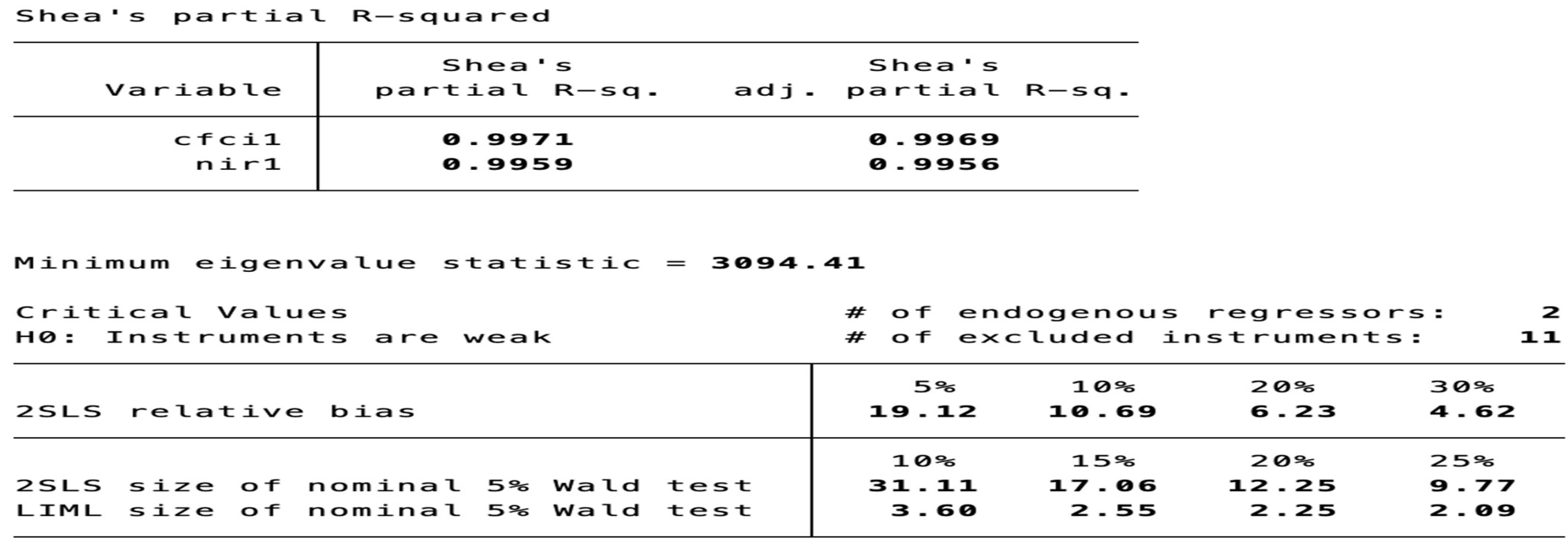
For an excluded exogenous variable to be a valid instrument, it must be sufficiently correlated with the included endogenous regressors while remaining uncorrelated with the error term.
Figure A5. IS curve.
Forecasting 08 00051 g0a5
We use the Stock and Yogo weak-instrument test. The null hypothesis is that the set of instruments is weak. If we are willing to tolerate a 5% relative bias, we can conclude that our instruments are not weak because the test statistic of 394.41 exceeds the critical value of 19.12.
Using a Wald test at the 5% level, suppose that we are willing to accept a rejection rate of at most 10%. Because 394.41 > 31.11, we reject the null hypothesis of weak instruments.
Accordingly, using Shea’s adjusted partial R2 values are very high.
Figure A6. Phillips Curve.
Forecasting 08 00051 g0a6
The F-statistic for the joint significance of the coefficients on the additional instruments is significant and exceeds 10, meaning that the additional instruments have significant explanatory power for our endogenous regressors.
Stock and Yogo Weak-Instruments Test (Craig and Donald Minimum Eigen Statistic).
The null hypothesis of the Stock and Yogo test is that the set of instruments is weak. Choosing the highest relative bias, we are willing to tolerate 5%, we can see that the test statistic exceeds the critical value; hence, we conclude that our instruments are not weak.
Figure A7. Financial cycle.
Forecasting 08 00051 g0a7
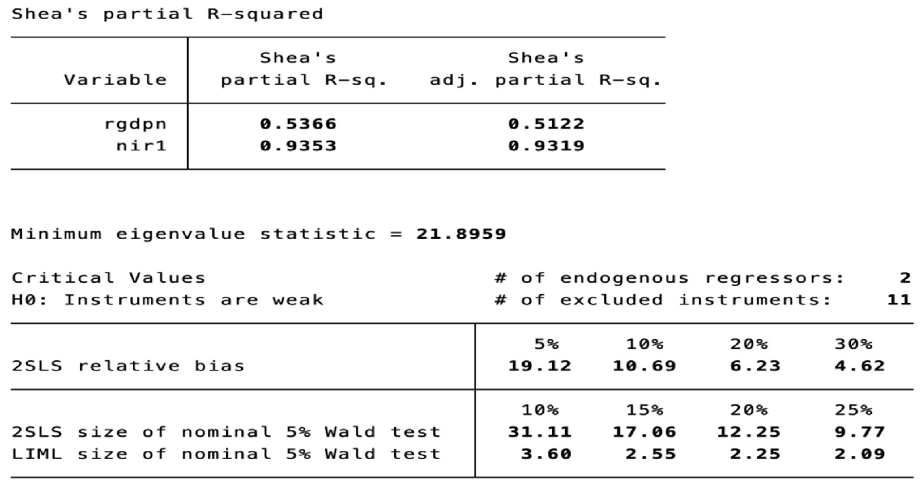
Shea’s adjusted partial R2 is high for the nominal interest rate and above 50% for the real GDP gap.
Stock and Yogo Weak-Instruments Test (Craig and Donald Minimum Eigen Statistic).
The null hypothesis of the Stock and Yogo test is that the set of instruments is weak. Choosing the highest relative bias, we are willing to tolerate 5%, we can see that the minimum eigen test statistic (21.8959) exceeds the critical value (19.12); hence, we conclude that our instruments are not weak.
Figure A8. Monetary policy rule.
Forecasting 08 00051 g0a8
F-Statistic
The F-statistic for the joint significance of the coefficients on the additional instruments are significant and exceed 10, meaning that the additional instruments have significant explanatory power for our endogenous regressors.
Stock and Yogo Weak-Instruments Test (Craig and Donald Minimum Eigen Statistic).
The null hypothesis of the Stock and Yogo test is that the set of instruments is weak. Choosing the highest relative bias, we are willing to tolerate 5%, we can see that the test statistic exceeds the critical value; hence, we conclude that our instruments are not weak.

References

  1. Kydland, F.E.; Prescott, E.C. Time to build and aggregate fluctuations. Econom. J. Econom. Soc. 1982, 50, 1345–1370. [Google Scholar] [CrossRef] [Scilit]
  2. Long, J.B., Jr.; Plosser, C.I. Real business cycles. J. Political Econ. 1983, 91, 39–69. [Google Scholar] [CrossRef] [Scilit]
  3. Ma, Y.; Zhang, J. Financial Cycle, Business Cycle and Monetary Policy: Evidence from Four Major Economies. Int. J. Financ. Econ. 2016, 21, 502–527. [Google Scholar] [CrossRef] [Scilit]
  4. Gurley, J.G.; Shaw, E.S. Financial aspects of economic development. Am. Econ. Rev. 1955, 45, 515–538. [Google Scholar] [CrossRef]
  5. Kindleberger, C.P.; Kindleberger, C.P. Economic Response: Comparative Studies in Trade, Finance, and Growth; Harvard University Press: Cambridge, MA, USA, 1978. [Google Scholar]
  6. Minsky, H.P. The Financial Instability Hypothesis; Working Paper No. 74; The Jerome Levy Economics Institute: Annandale-on-Hudson, NY, USA, 1992. [Google Scholar]
  7. Adrian, T.; Liang, N. Monetary Policy, Financial Conditions, and Financial Stability. 2016. Available online: https://ssrn.com/abstract=2811090 (accessed on 1 June 2026).
  8. Godwin, A.; Howse, T.; Ramsey, I. Twin peaks: South Africa’s financial sector regulatory framework. S. Afr. Law J. 2017, 134, 665–702. [Google Scholar]
  9. Ajello, A.; Goldberg, J.; Perez-Orive, A. Which Financial Shocks Drive the Business Cycle? Manuscript, Federal Reserve Board Technical Report; Federal Reserve Board: Washington, DC, USA, 2018. [Google Scholar]
  10. Fadeyi, O.A.; Sedibe, M.M.; van der Westhuizen, C.; Igene, L. Financial crisis and the South African agricultural sector: A computable general equilibrium (CGE) analysis. Afr. J. Bus. Econ. Res. 2019, 14, 71. [Google Scholar] [CrossRef] [Scilit]
  11. Ndlela, T.; Nkala, P. A structural analysis of the sources and dynamics of macroeconomic fluctuations in the South African economy. In TIPS Annual Forum; University of Cape Town: Cape Town, South Africa, 2003; pp. 8–10. [Google Scholar]
  12. Redl, C. Macroeconomic uncertainty in south africa. S. Afr. J. Econ. 2018, 86, 361–380. [Google Scholar] [CrossRef] [Scilit]
  13. Fuat Yıldız, B.; Hesami, S.; Rjoub, H.; Wong, W.-K. Interpretation of oil price shocks on macroeconomic aggregates of South Africa: Evidence from SVAR. J. Contemp. Issues Bus. Gov. 2021, 27, 279–287. [Google Scholar]
  14. Christensen, I.; Dib, A. The financial accelerator in an estimated New Keynesian model. Rev. Econ. Dyn. 2008, 11, 155–178. [Google Scholar] [CrossRef] [Scilit]
  15. Hirakata, N.; Sudo, N.; Ueda, K. Do banking shocks matter for the US economy? J. Econ. Dyn. Control 2011, 35, 2042–2063. [Google Scholar] [CrossRef] [Scilit]
  16. Jermann, U.; Quadrini, V. Macroeconomic effects of financial shocks. Am. Econ. Rev. 2012, 102, 238–271. [Google Scholar] [CrossRef] [Scilit]
  17. Iacoviello, M. Financial business cycles. Rev. Econ. Dyn. 2015, 18, 140–163. [Google Scholar] [CrossRef] [Scilit]
  18. Ajello, A. Financial intermediation, investment dynamics, and business cycle fluctuations. Am. Econ. Rev. 2016, 106, 2256–2303. [Google Scholar] [CrossRef] [Scilit]
  19. Claessens, S.; Kose, M.A.; Terrones, M.E. How do business and financial cycles interact? J. Int. Econ. 2012, 87, 178–190. [Google Scholar] [CrossRef] [Scilit]
  20. King, R.G.; Rebelo, S.T. Resuscitating real business cycles. In Handbook of Macroeconomics; Elsevier: Amsterdam, The Netherlands, 1999; Volume 1, pp. 927–1007. [Google Scholar]
  21. Galí, J. On the role of technology shocks as a source of business cycles: Some new evidence. J. Eur. Econ. Assoc. 2004, 2, 372–380. [Google Scholar] [CrossRef] [Scilit]
  22. Fisher, J.D. The dynamic effects of neutral and investment-specific technology shocks. J. Political Econ. 2006, 114, 413–451. [Google Scholar] [CrossRef] [Scilit]
  23. Nyati, M.C. Should Monetary Policy in South Africa Lean against the Wind by Targeting the Financial Cycle? Economies 2024, 12, 145. [Google Scholar] [CrossRef] [Scilit]
  24. Nyati, M.; Msomi, S. Macroprudential and Monetary Policies in South Africa, Complements or Substitutes? Int. J. Res. Bus. Soc. Sci. (2147-4478) 2025, 14, 211–228. [Google Scholar] [CrossRef] [Scilit]
  25. Justiniano, A.; Primiceri, G.E.; Tambalotti, A. Investment shocks and business cycles. J. Monet. Econ. 2010, 57, 132–145. [Google Scholar] [CrossRef] [Scilit]
  26. Smets, F. Financial stability and monetary policy: How closely interlinked? Int. J. Cent. Bank. 2014, 10, 263–300. [Google Scholar]
  27. Bezemer, D.; Samarina, A.; Zhang, L. A New Data Set on Differentiated Credit; University of Groningen: Groningen, The Netherlands, 2016. [Google Scholar]
  28. Hollander, H. Macroprudential policy with convertible debt. J. Macroecon. 2017, 54, 285–305. [Google Scholar] [CrossRef] [Scilit]
  29. Hollander, H.; Van Lill, D. A Review of the South African Reserve Bank’s Financial Stability Policies; Department of Economics, Stellenbosch University: Stellenbosch, South Africa, 2019. [Google Scholar]
  30. Kiyotaki, N.; Moore, J. Liquidity, business cycles, and monetary policy. J. Political Econ. 2019, 127, 2926–2966. [Google Scholar] [CrossRef] [Scilit]
  31. Magubane, K. Financial cycles synchronisation in South Africa. A dynamic conditional correlation (DCC) Approach. Cogent Econ. Financ. 2024, 12, 2321069. [Google Scholar] [CrossRef] [Scilit]
  32. Magubane, K. The stability of the financial cycle: Insights from a Markov switching regression in South Africa. J. Risk Financ. Manag. 2025, 18, 76. [Google Scholar] [CrossRef] [Scilit]
  33. Christiano, L.; Rostagno, M.; Motto, R. Financial Factors in Economic Fluctuations; ECB Working Paper; European Central Bank (ECB): Frankfurt am Main, Germany, 2010. [Google Scholar]
  34. Hafstead, M.; Smith, J. Financial shocks, bank intermediation, and monetary policy in a DSGE model. Unpubl. Manucript 2012, 9, 1–77. [Google Scholar]
  35. Mandelman, F.S. Business cycles and monetary regimes in emerging economies: A role for a monopolistic banking sector. J. Int. Econ. 2010, 81, 122–138. [Google Scholar] [CrossRef] [Scilit]
  36. Shahrour, M.H.; Arouri, M.; Rao, S. Linking climate risk to credit risk: Evidence from sectorial analysis. J. Altern. Invest. 2025, 27, 118–135. [Google Scholar]
  37. Caldara, D.; Fuentes-Albero, C.; Gilchrist, S.; Zakrajšek, E. The macroeconomic impact of financial and uncertainty shocks. Eur. Econ. Rev. 2016, 88, 185–207. [Google Scholar] [CrossRef] [Scilit]
  38. Christiano, L.; Ikeda, D. Leverage Restrictions in a Business Cycle Model; National Bureau of Economic Research: Cambridge, MA, USA, 2013. [Google Scholar]
  39. Goodhart, C.; Hofmann, B. The IS curve and the transmission of monetary policy: Is there a puzzle? Appl. Econ. 2005, 37, 29–36. [Google Scholar] [CrossRef] [Scilit]
  40. Scheibe, J.; Vines, D. A Phillips Curve for China. 2005. Available online: https://ssrn.com/abstract=770244 (accessed on 1 June 2026).
  41. Taylor, J.B.; Williams, J.C. Simple and robust rules for monetary policy. In Handbook of Monetary Economics; Elsevier: Amsterdam, The Netherlands, 2010; Volume 3, pp. 829–859. [Google Scholar]
  42. Verona, F.; Martins, M.M.; Drumond, I. Financial shocks, financial stability, and optimal Taylor rules. J. Macroecon. 2017, 54, 187–207. [Google Scholar] [CrossRef] [Scilit]
  43. Krznar, M.I.; Matheson, M.T.D. Financial and Business Cycles in Brazil; International Monetary Fund: Washington, DC, USA, 2017. [Google Scholar]
  44. Chorafas, D.N. Financial Cycles; Springer: Berlin/Heidelberg, Germany, 2015; pp. 1–24. [Google Scholar]
  45. Kim, C.-J. Dynamic linear models with Markov-switching. J. Econom. 1994, 60, 1–22. [Google Scholar] [CrossRef] [Scilit]
  46. Kim, M.-J.; Yoo, J.-S. New index of coincident indicators: A multivariate Markov switching factor model approach. J. Monet. Econ. 1995, 36, 607–630. [Google Scholar] [CrossRef] [Scilit]
  47. Doz, C.; Petronevich, A. Dating Business Cycle Turning Points for the French Economy: An MS-DFM approach. In Dynamic Factor Models; Emerald Group Publishing Limited: Leeds, UK, 2016; pp. 481–538. [Google Scholar]
  48. Hamilton, J.D. A new approach to the economic analysis of nonstationary time series and the business cycle. Econom. J. Econom. Soc. 1989, 57, 357–384. [Google Scholar] [CrossRef] [Scilit]
  49. Bosch, A.; Ruch, F. An Alternative Business Cycle Dating Procedure for S outh A frica. S. Afr. J. Econ. 2013, 81, 491–516. [Google Scholar] [CrossRef] [Scilit]
  50. Krznar, I. Identifying Recession and Expansion Periods in Croatia; Working Pepers W-29; Croatian National Bank: Zagreb, Croatia, 2011. [Google Scholar]
  51. Drehmann, M.; Borio, C.E.; Tsatsaronis, K. Characterising the Financial Cycle: Don’t Lose Sight of the Medium Term! 2012. Available online: https://ssrn.com/abstract=2084835 (accessed on 1 June 2026).
  52. Hansen, L.P. Generalized method of moments estimation. In Macroeconometrics and Time Series Analysis; Springer: Berlin/Heidelberg, Germany, 2010; pp. 105–118. [Google Scholar]
  53. Hansen, L.P. Large sample properties of generalized method of moments estimators. Econom. J. Econom. Soc. 1982, 50, 1029–1054. [Google Scholar] [CrossRef] [Scilit]
  54. Hall, A.R. Econometricians have their moments: GMM at 32. Econ. Rec. 2015, 91, 1–24. [Google Scholar] [CrossRef] [Scilit]
  55. Hansen, L.P. Generalized method of moments estimation. In The New Palgrave Dictionary of Economics; Palgrave Macmillan: London, UK, 2018; pp. 5201–5211. [Google Scholar]
  56. Molodtsova, T.; Papell, D.H. Out-of-sample exchange rate predictability with Taylor rule fundamentals. J. Int. Econ. 2009, 77, 167–180. [Google Scholar] [CrossRef] [Scilit]
  57. Hafner, C.M.; Lauwers, A.R. An augmented Taylor rule for the Federal Reserve’s response to asset prices. Int. J. Comput. Econ. Econom. 2017, 7, 115–151. [Google Scholar]
  58. Borio, C. The financial cycle and macroeconomics: What have we learnt? J. Bank. Financ. 2014, 45, 182–198. [Google Scholar] [CrossRef] [Scilit]
  59. Gupta, R.; Hollander, H.; Steinbach, R. Forecasting output growth using a DSGE-based decomposition of the South African yield curve. Empir. Econ. 2020, 58, 351–378. [Google Scholar]
  60. Steinbach, M.; Mathuloe, P.; Smit, B. An open economy New Keynesian DSGE model of the South African economy. S. Afr. J. Econ. 2009, 77, 207–227. [Google Scholar] [CrossRef] [Scilit]
  61. Tovar, C.E. DSGE models and central banks. Economics 2009, 3, 1–31. [Google Scholar] [CrossRef] [Scilit]
  62. Junior, C.J.C. Understanding DSGE Models: Theory and Applications; Vernon Press: Wilmington, DE, USA, 2016. [Google Scholar]
  63. Calvo, G.A. Staggered prices in a utility-maximizing framework. J. Monet. Econ. 1983, 12, 383–398. [Google Scholar] [CrossRef] [Scilit]
  64. Smets, F.; Wouters, R. An estimated dynamic stochastic general equilibrium model of the euro area. J. Eur. Econ. Assoc. 2003, 1, 1123–1175. [Google Scholar] [CrossRef] [Scilit]
  65. Adolfson, M.; Laséen, S.; Lindé, J.; Villani, M. Bayesian estimation of an open economy DSGE model with incomplete pass-through. J. Int. Econ. 2007, 72, 481–511. [Google Scholar] [CrossRef] [Scilit]
  66. Smets, F.; Wouters, R. Shocks and frictions in US business cycles: A Bayesian DSGE approach. Am. Econ. Rev. 2007, 97, 586–606. [Google Scholar] [CrossRef] [Scilit]
  67. Clarida, R.; Gali, J.; Gertler, M. The science of monetary policy: A new Keynesian perspective. J. Econ. Lit. 1999, 37, 1661–1707. [Google Scholar] [CrossRef] [Scilit]
  68. Nyati, M.C.; Muzindutsi, P.-F.; Tipoy, C.K. Macroprudential and monetary policy interactions and coordination in South Africa: Evidence from business and financial cycle synchronisation. Economies 2023, 11, 272. [Google Scholar] [CrossRef] [Scilit]
  69. Liu, G.; Gupta, R. A small-scale DSGE model for forecasting the South African economy. S. Afr. J. Econ. 2007, 75, 179–193. [Google Scholar]
  70. Liu, G.; Molise, T. The optimal monetary and macroprudential policies for the South African economy. S. Afr. J. Econ. 2020, 88, 368–404. [Google Scholar] [CrossRef] [Scilit]
  71. Nyathi, M.C.; Tipoy, C.K.; Muzindutsi, P.F. Measuring and Testing a Modified Version of the South African Financial Cycle: Working Paper 869; Economic Research Southern Africa: Cape Town, South Africa, 2021. [Google Scholar]
  72. Kydland, F.E.; Zarazaga, C.E. Argentina’s lost decade. Rev. Econ. Dyn. 2002, 5, 152–165. [Google Scholar] [CrossRef] [Scilit]
  73. Botha, B.; Burger, R.; Kotze, K.; Rankin, N.; Steenkamp, D. Big data forecasting of South African inflation. Empir. Econ. 2022, 65, 149–188. [Google Scholar] [CrossRef] [Scilit] [PubMed]
  74. Fedderke, J.W.; Liu, W. Modelling the determinants of capital flows and capital flight: With an application to South African data from 1960 to 1995. Econ. Model. 2002, 19, 419–444. [Google Scholar] [CrossRef] [Scilit]
  75. Farrell, G.; Kemp, E. Measuring the financial cycle in South Africa. S. Afr. J. Econ. 2020, 88, 123–144. [Google Scholar] [CrossRef] [Scilit]
  76. Terrones, M.M.; Claessens, M.S.; Kose, M.A. How Do Business and Financial Cycles Interact? International Monetary Fund: Washington, DC, USA, 2011. [Google Scholar]
  77. Borio, C.E. Monetary Policy and Financial Stability: What Role in Prevention and Recovery? BIS: Basel, Switzerland, 2014. [Google Scholar]
  78. Rünstler, G.; Vlekke, M. Business and Financial Cycles: An Unobserved Components Models Perspective; European Central Bank (ECB): Frankfurt am Main, Germany, 2015. [Google Scholar]
  79. Claessens, S.; Valencia, F. The Interaction Between Monetary and Macroprudential Policies; IMF: Washington, DC, USA, 2013. [Google Scholar]
  80. Akar, C. Analyzing the synchronization between the financial and business cycles in Turkey. J. Rev. Glob. Econ. 2016, 5. Available online: https://ssrn.com/abstract=2913550 (accessed on 1 June 2026). [CrossRef] [Scilit]
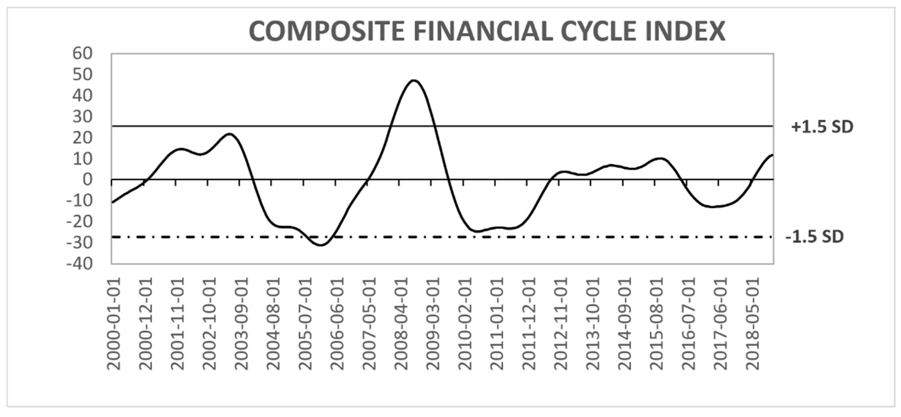
Figure 1. DFM-SSF financial cycle index. Source: Authors’ own estimates.
Forecasting 08 00051 g001
Figure 5. Response of endogenous variables to a positive financial cycle shock. Source: Authors’ depiction.
Forecasting 08 00051 g005
Table 1. CFCI dates at peaks and troughs.
CFCI
PeaksTroughs
May 2003January 2006
September 2008June 2011
Source: Author’s own estimates.
Table 2. GMM estimations of the extended hybrid IS curve.
Dependent Variabley
y t + 1 0.506 ***
(0.003)
y t 1 0.499 ***
(0.003)
r i r t + 1 −0.002 **
(0.000)
c f c i 0.007 ***
(0.000)
J-statistic (p-value) 13.463
(0.0873)
Note: Significance at the 5%, and 1% levels is reported by **, and ***, respectively. Source: Authors’ estimates (2026). Standard errors in parentheses.
Table 3. Multiple-equation GMM estimation of the four-equation model.
EquationParameterDescriptionValueJ-Statistic
(p-Value)
Extended IS curve y t = μ E t y t + 1 + α 1 y t 1 + β 1 ( r t E t π t + 1 ) + β 2 F C t + ε t y 81.978
(0.0665)
The J-test p-value is marginally significant. While above 0.05, it is sufficiently close to warrant conservative interpretation. See Section 2.3 Discussion.
μ Lead of the output gap0.510 *** (0.003)
α 1 Lag of the output gap0.494 *** (0.000)
β 1 Lead of the real interest rate gap−0.013 ** (0.010)
β 2 Composite FC index0.022 *** (0.000)
Phillips Curve π t = β 1 E π t + 1 + ( 1 β 1 ) π t 1 + β 2 y t + ε t π
β 1 Lead of the inflation gap0.512 *** (0.003)
1 β 1 Lag of the inflation gap0.503 *** (0.003)
β 2 Output gap0.029 *** (0.005)
Financial cycle C F C I t = θ 1 F C t 1 + θ 2 y t + θ 3 r t + ε t C F C I
θ 1 Lag of CFCI0.002 *** (0.000)
θ 2 Output gap1.234 *** (0.000)
θ 3 Nominal interest rate−0.258 *** (0.000)
Monetary policy r t = 0 + 1 π t + k + 2 y t + p + i = 1 p ρ i r t i + ε t
ρ i Interest rate smoothing0.848 *** (0.013)
1 Forward-looking inflation gap0.002 *** (0.000)
2 Forward-looking output gap1.686 *** (0.091)
Note: Significance at the 5%, and 1% levels is reported by **, and ***, respectively. Standard errors are in parentheses. Source: Authors’ estimates (2021).
Table 4. Calibration of model parameters.
ParameterDescriptionValueSource or Rationale
β Discount factor0.985Smets & Wouters (2003) [64]; SARB policy reports
σ Intertemporal elasticity of substitution (inverse of risk aversion)1.0Adolfson et al. (2007) [65]; Smets & Wouters (2003) [64]
h Habit persistence in consumption0.7Smets & Wouters (2007) [66]; Kydland & Zarazaga (2002) [72]
φ Weight of the output gap in the marginal cost1.5Calibrated to match the slope of NKPC; small-open-economy studies for SA (Botha, 2021) [73]
α Capital share in production0.33SA national accounts; Fedderke (2002) [74]
δ Depreciation rate0.025Standard in macro models (Smets & Wouters, 2003) [64]
ε p Elasticity of substitution among goods6Clarida, Galí & Gertler (1999) [67]; SA manufacturing estimates
θ p Calvo price stickiness0.75Smets & Wouters (2003) [64]; Botha (2021) [73]
κ ( c f c i ) Financial cycle amplification coefficient1.092Estimated by Nyati & Muzindutsi (2023) [68] baseline
ρ ( c f c i ) Persistence of the financial cycle0.924Nyati & Muzindutsi (2023) [68]; SA credit cycle estimates
θ ( c f c i ) Sensitivity of the financial cycle to the real rate−0.045Calibrated to reproduce observed counter-cyclicality
ρ r Interest rate smoothing0.6SARB Quarterly Bulletin; empirical Taylor rule estimates
ρ _ π Inflation response in the Taylor rule1.2SARB policy estimates; Clarida et al. (1999) [67]
ρ _ y Output gap response in the Taylor rule0.198Calibrated to SA VAR evidence (Botha, 2021) [73]
ρ _ f c _ m p Direct response to the financial cycle0.0Policy experiment parameter (Nyati & Muzindutsi 2023) [68]
ρ _ z Technology shock persistence0.9Standard value (Smets & Wouters, 2003) [64]
ρ _ y f o r Foreign output persistence0.9IMF WEO data; small-open-economy DSGE norms
ρ _ p i f o r Foreign inflation persistence0.9IMF/World Bank CPI data
ω Weight of foreign sector influence0.3SARB and IMF data
p a r a m s s
_ i _ o v e r _ y
Steady state investment–output ratio0.20SARB Quarterly Bulletin
π * Steady state inflation rate0.005SARB inflation target (3–6%) midpoint
Source: Authors’ estimates (2025).
Table 5. Variance decomposition model 1—base Taylor rule.
e _ y e _ π e _ r e _ c f c i e _ z e _ i
r G D P _ g a p 50.265.563.3815.6725.660.00
I N F 2.311.830.160.5993.920.00
R I R 0.540.640.790.1692.860.00
C F C I 41.914.434.452.5346.120.00
K 0.890.090.111.411.2986.91
I 26.642.951.798.3113.6053.77
Source: Authors’ estimates (2025).
Table 6. Variance decomposition model 2—Taylor rule + fc.
e _ y e _ π e _ r e _ c f c i e _ z e _ i
r G D P _ g a p 50.045.553.4014.4226.920.00
I N F 2.561.810.180.6093.510.00
R I R 0.610.590.920.1993.410.00
F C 40.104.244.412.5147.810.00
K 1.040.110.131.441.6585.63
I 28.223.131.928.1315.1850.04
Source: Authors’ estimates (2025).
Disclaimer/Publisher’s Note: The statements, opinions and data contained in all publications are solely those of the individual author(s) and contributor(s) and not of MDPI and/or the editor(s). MDPI and/or the editor(s) disclaim responsibility for any injury to people or property resulting from any ideas, methods, instructions or products referred to in the content.