Forecasting Municipal Financial Distress in South Africa: A Machine Learning Approach

Highlights

What are the main findings?

• Machine learning (ML) using the National Treasury’s 13 financial health indicators forecasts one-year-ahead municipal financial distress.
• Liquidity, solvency, cash coverage, and employment deprivation are identified as key drivers of municipal financial distress.

What are the implications of the main findings?

• ML models can convert the oversight monitoring data into a practical early-warning tool for risk-based municipal oversight.
• The prioritisation of the highest-risk municipalities yields a short, actionable list for targeted support and earlier fiscal recovery action.

Abstract

Persistent fiscal stress in South African municipalities undermines service delivery, yet practical tools for early detection remain limited. This study predicts one-year-ahead municipal financial distress to support risk-based prioritisation. We develop machine learning models using a 2018/19–2022/23 municipality panel, combining 13 financial health indicators from State of Local Government (SoLG) reports with selected socio-economic variables. Penalised logistic regression is benchmarked against random forest and XGBoost under a leakage-aware, time-ordered split into training, validation, and an out-of-time test year; class imbalance is handled through class weighting. Performance is evaluated using PR-AUC, ROC-AUC, calibration, and a capacity-constrained Top-30 rule. All models outperform a naïve last-year baseline on the out-of-time test (PR-AUC 0.934–0.954; ROC-AUC 0.886–0.923), with bootstrap intervals supporting robustness. Random forest performs best overall, while penalised logistic regression remains competitive. Under the Top-30 rule (12.3% workload), precision is high (precision@30 0.967–1.000) while recall is modest (recall@30 0.186–0.192). SHAP values and logistic odds ratios identify liquidity, solvency, cash coverage, and employment deprivation as key drivers. The Top-30 rule corresponds to an annual intensive monitoring portfolio that is reasonable under constrained staffing and budget capacity in national and provincial oversight units, while probability thresholds are reported as conventional benchmarks rather than as policy triggers.

1. Introduction

The local government sphere in South Africa currently struggles with escalating and widespread financial distress, with several municipalities experiencing varying levels of fiscal strain while others are undergoing financial collapse [1,2]. This situation undermines the constitutional mandate for the provision of basic services and forces reactive interventions by other government sectors [3]. Despite the urgency, a gap remains in practical, predictive mechanisms that oversight institutions can apply to detect future financial distress. The current study addressed the operational need for proactive oversight by forecasting one-year-ahead municipal financial distress at the municipality-year level, producing ranked early-warning lists aligned to oversight capacity.

Financial distress denotes an impaired ability to meet financial and service delivery obligations sustainably, consistent with the statutory triggers under the MFMA ss. 138, 140 (see [4]) and operationalised using the 13-indicator framework under the South African National Treasury. Despite being widely applied to monitor fiscal health, this framework is retrospective and ratio-centred, with limited validation as a predictive early-warning tool and modest integration of socio-economic or governance dimensions [5,6,7]. Consequently, the South African local government lacks a calibrated, time-aware predicting workflow that translates routine indicators into actionable signals for planning and support.

The literature highlighted that effective early warning systems (EWSs) are designed to identify municipalities in distress and to forecast potential distress expeditiously for timely intervention. An effective EWS focuses on predictive modelling, multi-dimensional indicators, governance awareness, timely data, and transparent escalation mechanisms [8,9]. In New York (USA) [10] and East Java, Indonesia [11], these features help governments act earlier, reduce costs, and protect service delivery. The current South African practice remains restricted and significantly retrospective relative to these standards, reinforcing the need for a validated forecasting approach that provides calibrated probabilities and practical operating thresholds.

The recent machine learning (ML) applications to local government fiscal distress are limited (five studies across Spain, Italy, China, and the United States), displaying several constraints: metrics often emphasise accuracy or F1 over early-warning-relevant measures, with only two studies reporting precision–recall (PR) curves. Furthermore, class imbalance is disregarded or managed using simple oversampling, undersampling, or class weights. Validation relies on random splits or random cross-validation without time or group blocking. Interpretability is minimal (lists of significant variables or generic importance, with one study using an expert-driven feature set). Finally, contextual fit varies, as designs are tailored to specific countries or city sizes rather than portable workflows [12,13,14,15,16].

These shortcomings were addressed by developing and comparing three tabular data models tailored to public finance oversight: a transparent penalised logistic regression, random forest, and XGBoost. Models were trained during earlier financial years, tuned using a held-out validation year, and evaluated on an out-of-time test year, respecting temporal ordering and supporting leakage-resistant assessment [17,18]. Class weighting was employed considering the class imbalance (including scale_pos_weight for XGBoost). Evaluation prioritised PR-AUC (primary) and recall@K (with K linked to programme capacity; see Kleinberg et al. [19]), alongside ROC-AUC, the F1-score for the distressed class, and the calibration, which was assessed using the Brier score and reliability curves [20]. Interpretability combined odds ratios for penalised logistic regression with SHAP-based explanations for the XGBoost model, which provided a single, coherent set of non-linear attributions via summary and dependence plots [21].

The primary study objective was to develop and evaluate models that predict one-year-ahead municipal financial distress in South Africa using routinely collected financial, governance, and service delivery indicators within a calibrated, time-aware workflow. The objective was achieved by addressing these two questions:

• Which indicators contribute most to the models’ predicted distress risk?
• How do penalised logistic regression, random forest, and XGBoost models compare to PR-AUC, recall@K, ROC-AUC, and calibration?

This study makes four contributions by addressing the limitations in prior local government ML studies. First, a calibrated early-warning workflow was presented, implementable with routinely available data. Second, capacity-linked thresholds (recall@K) were operationalised to convert probabilities into manageable action lists. Third, policy legibility was maintained through outputs that were interpretable and suitable for governance contexts. Fourth, the current study quantified uncertainty via bootstrap confidence intervals on key performance metrics, enabling risk-aware interpretation of early-warning model performance.

The remainder of the study is structured as follows: Section 2 discusses the relevant literature and research gap. Section 3 outlines the methodology and model development process. Furthermore, Section 4 demonstrates the model performance results, while Section 5 discusses the results, policy implications, and conclusions.

2. Literature Review

2.1. Challenges in Predicting Municipal Financial Distress

Research on financial distress prediction in local governments lags behind that in the corporate sector, which impedes efforts to develop robust predictive models [22]. Predicting municipal financial distress is hindered by conceptual heterogeneity (varying definitions and measures of the phenomenon of “financial distress”), which undermines the comparability and portability of models across jurisdictions [23,24]. Another recurring challenge is class imbalance, whereby several distressed cases bias learning and inflate apparent accuracy while masking false negatives, diminishing early-warning value [13,25]. The third challenge concerns validation design, where various studies rely on random train–test splits or in-sample or retrospective fits. This practice risks temporal leakage and inflates reported performance [26].

Considering that several municipal FDP models employ historical data without testing on contemporary or out-of-time datasets, their cross-context applicability is limited [27]. Interpretability remains a persistent flaw in local government FDP models, limiting their policy and rarely yielding actionable insights for officials and decision-makers [14,28]. Calibration and decision rules are seldom reported in FDP studies, and poor calibration or ad hoc thresholds can mislead interpretation and action [24,29]. Moreover, subjective cut-offs and poorly calibrated scores usually create false reassurance or unwarranted alarm [30,31].

2.2. The Application of Machine Learning for the Prediction of Municipal Financial Distress

Recent applications of ML to municipal finance distress prediction display progress, but several shortcomings limit their generalisation to other contexts. Although Alaminos et al. [12] demonstrated feasibility, they relied on accuracy-only metrics and excluded class imbalance, thereby providing limited interpretability beyond identifying significant variables. Antulov-Fantulin et al. [13] expanded the feature set and applied oversampling or class weights with ROC/PR evaluation. Nonetheless, their validation strategy employed random splits rather than time-aware blocking, which increased the risk of temporal leakage. Li et al. [14] integrated econometric proxies with ML but provided limited interpretability, which was confined to proxy-level insights. Their models were evaluated primarily for general risk classification instead of actionable municipal thresholds.

Piermarini et al. [15] employed expert-driven feature extraction for their ML models, which were assessed using F1-scores and precision–recall curves without calibration or uncertainty assessment, thereby limiting broader applicability. Liu et al. [16] improved minority class detection via undersampling and bagging. Nonetheless, F1 was prioritised as the key metric, and the study did not incorporate calibration, decision thresholds, or interpretability beyond variable importance.

Table 1. Methodological comparison of municipal ML studies.

Study	Metric Used	Imbalance Handling	Validation Design	Interpretability	Contextual Fit
Alaminos et al. [12] (Spain)	Accuracy only	Not addressed	Random train/test split	Limited (list of significant variables)	Spain, large cities
Antulov-Fantulin et al. [13] (Italy)	ROC, PR	Oversampling	Random CV, no blocking	Basic feature importance	Italy, all municipalities
Li et al. [14] (China)	Accuracy, general risk classification	Not explicit (risk proxies via CRITIC, MS-AR)	Not explicit	Proxy-level only	Chinese provincial debt risk
Piermarini et al. [15] (Italy)	F1, PR curves	Class weights	Five-fold CV, random splits	Expert-driven feature extraction	Italy, aligned with the audit criteria
Liu et al. [16] (United States)	F1, accuracy, recall, precision	Undersampling (majority, optimal ratio)	Five-fold CV, random splits	Variable importance only	US, 49 states, LGs

presents the methodological comparison of recent machine learning studies predicting municipal financial distress (metrics, imbalance handling, validation design, interpretability, and contextual fit).

These past studies illustrate the trajectory of municipal FDP research, shifting from ratio-based indices towards ML models that address imbalance and expand feature sets. Nonetheless, methodological gaps were identified, including ad hoc imbalance handling, non-temporal validation, uncommon calibration, and decision thresholds rarely linked to operational capacity.

2.3. Emerging Machine Learning Solutions to the FDP Challenges

Recent ML developments offer practical remedies to the abovementioned shortcomings of municipal FDP. Class imbalance can be managed with class weights or Synthetic Minority Oversampling Technique (SMOTE) variants [32]. Validation has shifted towards temporal and group-blocked cross-validation with external holdouts [17]. Meanwhile, interpretability can be enhanced using SHAP values, model coefficients, and partial dependence plots [33,34]. Calibration and decision rules benefit from isotonic or Platt scaling with Brier scores and reliability curves [35,36]. Additionally, robustness can be probed via simple bootstrapping and sensitivity checks. Nevertheless, these approaches remain underutilised in municipal FDP studies. Section 3 of this study operationalises these techniques in detail.

2.4. Research Gap and Contribution

Recent applications of ML to municipal financial distress prediction have demonstrated improved predictive performance. Nonetheless, the scope is limited, as observed in these gaps: (i) imbalance is managed inconsistently and rarely benchmarked against class-weighted baselines, (ii) validation commonly utilises random splits, overstating performance, (iii) interpretability and calibration are under-reported, limiting safe deployment, and (iv) contextual fit remains narrow, with limited integration of governance or socio-economic indicators and modest portability to developing country settings.

The present study addressed these gaps by (i) comparing a transparent penalised logistic regression model with random forest and XGBoost models under a leakage-resistant, time-aware validation design that respects temporal ordering and municipality grouping, (ii) managing class imbalance through class weighting rather than synthetic oversampling, (iii) evaluating performance using PR-AUC as the primary metric, complemented by ROC-AUC, the F1-score for the distressed class, calibration diagnostics (Brier score and reliability curves), and recall at a capacity-relevant top-K threshold, and (iv) providing policy-legible explanations through penalised-logit odds ratios and SHAP-based interpretation of the tree-based model(s) using South African municipal data aligned with the SoLG/NT-13 framework of the South African National Treasury.

3. Materials and Methods

A quantitative, longitudinal research design was employed using supervised ML methods. The primary task was binary classification to predict whether a municipality is financially distressed. The design was based on design science research and informed by institutional, signalling, and resource dependence theories.

3.1. Overview of the Modelling Pipeline

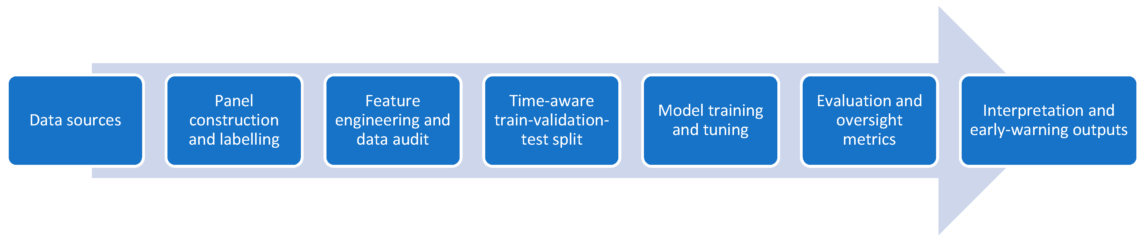
Figure 1 summarises the overall modelling pipeline, including data assembly and feature construction, as well as model training, evaluation, and interpretation.

At a high level, the workflow proceeded from assembling an integrated municipality-year panel and constructing financial, socio-economic, governance, and environmental indicators. Subsequently, the distress outcome was defined, and the data were divided into temporally ordered training, validation, and test sets, with three prediction models (penalised logistic regression, random forest, and XGBoost). Finally, their one-year-ahead early-warning performance was evaluated and interpreted.

3.2. Data Sources and Panel Construction

The empirical analysis employed a balanced municipality-year panel for all 257 South African municipalities from 2018/19 to 2022/23, yielding 1285 observations. These years aligned with the consistent application of the 13-indicator financial health framework of the South African National Treasury. Municipality codes and financial-year labels were harmonised as unique keys, ensuring specifically one record per municipality-year with no missing identifiers and no duplicate combinations.

The panel combined information from several administrative and statistical sources. These financial indicators were obtained from the National Treasury: the Local Government Database and Reporting System (LGDRS)/Municipal Standard Chart of Accounts (mSCOA) datasets and Section 71 returns, supplemented with Auditor-General outputs, Community Survey 2016 and Census 2022 population demographics [37,38] and South African Index of Multiple Deprivation (SAIMD) 2022 deprivation indices, and provincial macro-economic series (GDP-R, CPI inflation and unemployment) aligned with the municipal financial year. Additionally, governance and political variables were compiled from election results, council composition records, and administrative sources. The National Treasury outlined persistent discrepancies and occasional reporting errors in mSCOA uploads to the LGDRS relative to signed audited financial statements [2].

Table A1. Predictor dictionary: labels, indicator mapping, construction rules, and data sources.

Variable Dimension	Variable Label	Indicator	Formula or Construction	Source Dataset
Cash solvency	Cash or Cash-Equivalent Position Less Applications	Cash and cash equivalents available for operations after deducting committed applications (unspent conditional grants, statutory commitments)	Cash and cash equivalents—cash-backed committed funds	AFS/NT Local Government Database (mSCOA)
	Cash Plus Investments	Total immediately available liquid resources (cash plus investments)	Cash and cash equivalents + investments	AFS/NT Local Government Database (mSCOA)
	Cash Coverage (Months)	Number of months that available cash can cover operating expenditure	(Cash and cash equivalents + investments − committed funds) ÷ (operating expenditure excluding depreciation and amortisation) ÷ 12	AFS/NT Local Government Database (mSCOA)
	Liquidity Ratio	Short-term liquidity; ability to meet current obligations	Current assets ÷ Current liabilities (as per AFS/NT definition)	AFS/NT Local Government Database (mSCOA)
	Current Ratio	Alternative short-term liquidity ratio reported by NT	Current assets ÷ current liabilities (reported as per NT circulars)	AFS/NT Local Government Database (mSCOA)
	Debtor Days	Average number of days to collect billed revenue from customers	(Trade and other receivables from exchange transactions ÷ total billed revenue) × 365	AFS/NT Local Government Database (mSCOA)
	Creditor Days	Average number of days taken to pay suppliers and other creditors	(Trade and other payables ÷ total operating expenditure) × 365	AFS/NT Local Government Database (mSCOA)
Budget solvency	Operating_Surplus_Abs_Audited	Absolute operating surplus or deficit based on audited financial statements	Total operating revenue—total operating expenditure (audited)	AFS/NT Local Government Database (mSCOA)
Budget solvency	Operating_Surplus_Pct_Audited	Operating surplus as a percentage of operating revenue	(Operating_Surplus_Abs_Audited ÷ total operating revenue) × 100	AFS/NT Local Government Database (mSCOA)
Budget solvency	Opex_to_Revenue	Operating expenditure as a share of operating revenue (primary source)	Total operating expenditure ÷ total operating revenue (from main NT dataset)	AFS/NT Local Government Database (mSCOA)
Service-level solvency	FBS_Water_Coverage	Coverage of free basic water among domestic consumer units	Domestic FBS water consumer units ÷ total domestic water consumer units	NT Local Government Database (mSCOA FBS indicators)
	FBS_Elec_Coverage	Coverage of free basic electricity among domestic consumer units	Domestic FBS electricity consumer units ÷ total domestic electricity consumer units	NT Local Government Database (mSCOA FBS indicators)
	FBS_Sanitation_Coverage	Coverage of free basic sanitation among domestic consumer units	Domestic FBS sanitation consumer units ÷ total domestic sanitation consumer units	NT Local Government Database (mSCOA FBS indicators)
	FBS_Refuse_Coverage	Coverage of free basic refuse removal among domestic consumer units	Domestic FBS refuse consumer units ÷ total domestic refuse consumer units	NT Local Government Database (mSCOA FBS indicators)
	Pop. Density per km2	Population density in 2022; a proxy for service demand and settlement patterns	Total population 2022 ÷ land area (km2)	Stats SA Census 2022 and municipal GIS area data
	Density_Annual_Growth_2016_2022	Annualised growth rate of population density between 2016 and 2022	[(Density_2022 ÷ density_2016)^(1/6) − 1] × 100	Stats SA Census 2011 and 2022 (derived)
	Median_Age_2022	Median age of the municipal population in 2022	Median age as reported by Census 2022 (no further transformation)	Stats SA Census 2022
	Avg_HH_Size_2022	Average household size in 2022	Total population 2022 ÷ number of households 2022	Stats SA Census 2022
Long-term solvency	Repairs and Maintenance Expenditure Level (%)	Repairs and maintenance expenditure as a percentage of asset base	(Repairs and maintenance expenditure ÷ carrying value of property, plant, and equipment) × 100	AFS/NT Local Government Database (mSCOA)
Long-term solvency	Asset Renewal Rehabilitation Expenditure Level (%)	Share of capital expenditure devoted to asset renewal and rehabilitation	(Capital expenditure on renewal/rehabilitation ÷ total capital expenditure) × 100	AFS/NT Local Government Database (mSCOA)
Long-term solvency	Asset Renewal Depreciation Level (%)	Extent to which depreciation is covered by renewal expenditure	Capital expenditure on asset renewal ÷ depreciation × 100	AFS/NT Local Government Database (mSCOA)
Long-term solvency	CAPEX as PCT of Total Expenditure (%)	Capital expenditure as a share of total expenditure	Capital expenditure ÷ (operating expenditure + capital expenditure) × 100	AFS/NT Local Government Database (mSCOA)
Long-term solvency	Solvency Ratio	Overall solvency: ability to cover total liabilities with assets	Total assets ÷ total liabilities	AFS/NT Local Government Database (mSCOA)
Long-term solvency	Debt Total Borrowing vs. Total Operating Revenue	Level of interest-bearing borrowing relative to operating revenue	(Total interest-bearing borrowings ÷ total operating revenue) × 100	AFS/NT Local Government Database (mSCOA)
Long-term solvency	GF_Size	Size of general fund/accumulated surplus	Accumulated surplus (general fund) as reported in AFS	AFS/NT Local Government Database (mSCOA)
Long-term solvency	GF_to_Revenue	General fund relative to operating revenue	GF_Size ÷ total operating revenue	AFS/NT Local Government Database (mSCOA)
Long-term solvency	GF_to_OpEx	General fund relative to operating expenditure	GF_Size ÷ total operating expenditure	AFS/NT Local Government Database (mSCOA)
Long-term solvency	NetAssetRatio	Net assets as a share of total assets	Net assets ÷ total assets	AFS/NT Local Government Database (mSCOA)
Long-term solvency	Grants_Share	Dependence on operating grants and subsidies	Operating grants and subsidies revenue ÷ total operating revenue	AFS/NT Local Government Database (mSCOA)
Long-term solvency	Own_Revenue_Share	Share of operating revenue derived from own sources	Own revenue (rates, service charges, other own income) ÷ total operating revenue	AFS/NT Local Government Database (mSCOA)
Long-term solvency	Grants_per_capita	Operating grants and subsidies per capita	Operating grants and subsidies revenue ÷ total population	AFS/NT Local Government Database (mSCOA) and stats SA population
Long-term solvency	Own_Revenue_per_capita	Own revenue per capita	Own revenue ÷ total population	AFS/NT Local Government Database (mSCOA) and stats SA population
Long-term solvency	Total_OpEx_per_capita	Operating expenditure per capita	Total operating expenditure ÷ total population	AFS/NT Local Government Database (mSCOA) and stats SA population
Long-term solvency	BulkPurchases_Pct_OpEx	Bulk purchases and inventory consumed as a share of total operating expenditure	(Bulk purchases + inventory consumed) ÷ total operating expenditure	NT Local Government Database (mSCOA item codes)
Long-term solvency	Contracted_Services_Pct_Opex	Contracted services as a share of total operating expenditure	Contracted services ÷ total operating expenditure	NT Local Government Database (mSCOA item codes)
Additional governance indicators	Audit Outcome	Audit opinion of the municipality (proxy for financial management quality)	Categorical outcome as per Auditor-General (unqualified, qualified, adverse, disclaimed). Can be recoded as binary flag: 1 = qualified/adverse/disclaimed; 0 = unqualified (with or without findings)	Auditor-General reports/NT Local Government Database
Additional governance indicators	Budget_Funding_Position	Whether the municipal budget is funded in terms of MFMA funding compliance	Binary indicator: 1 = funded budget (NT funding criteria met); 0 = unfunded budget	NT budget funding assessments/Local Government Database
Additional governance indicators	UIFW_Total	Total unauthorised, irregular, fruitless, and wasteful expenditure incurred	Sum of unauthorised, irregular, fruitless, and wasteful expenditure as disclosed in AFS	AFS/NT Local Government Database (mSCOA)
Additional governance indicators	UIFW_to_OpEx	UIFW relative to operating expenditure	UIFW_Total ÷ total operating expenditure	AFS/NT Local Government Database (mSCOA)
Additional governance indicators	Unauth_to_OpEx	Unauthorised expenditure relative to operating expenditure	Unauthorised expenditure ÷ total operating expenditure	AFS/NT Local Government Database (mSCOA)
Additional governance indicators	Council_Control_Type	Political control configuration of the municipal council (single-party majority, coalition)	Categorical coding based on municipal election results and council composition	IEC election results, COGTA/municipal council records
Additional governance indicators	Mayor_Gender	Gender of the mayor (proxy for demographic diversity in political leadership)	Binary indicator: 1 = female mayor; 0 = male mayor	COGTA/municipal websites/council records
Additional governance indicators	Voter_Turnout_Pct	Voter turnout at municipal elections (proxy for electoral accountability)	(Valid votes cast ÷ registered voters) × 100, using 2016 and 2021 local election data mapped to financial years	IEC local government election results
Additional governance indicators	Water_Service_Provider	Institutional arrangement for water service provision (municipality vs. external provider)	Categorical variable indicating the main water service provider (municipality, water board, other)	COGTA/municipal service delivery arrangements/WSA records
Additional governance indicators	Electricity_Service_Provider	Institutional arrangement for electricity distribution	Categorical variable indicating the main electricity distributor (municipality, Eskom)	COGTA/municipal service delivery arrangements/NERSA/Eskom
Additional governance indicators	Sanitation_Service_Provider	Institutional arrangement for sanitation services	Categorical variable indicating the main sanitation service provider (municipality vs. external)	COGTA/municipal service delivery arrangements
Additional governance indicators	Refuse_Service_Provider	Institutional arrangement for refuse removal services	Categorical variable indicating the main refuse removal service provider	COGTA/municipal service delivery arrangements
Additional macro-economic indicators	SAIMD_Employment_Deprivation_2022	Employment deprivation index as a proxy for labour market-related poverty	SAIMD 2022 employment deprivation score (0–1) at the municipal level; used without transformation	SAIMD 2022 (Stats SA/SAMRC/partner institutions)
Additional macro-economic indicators	SAIMD_Education_Deprivation_2022	Education deprivation index	SAIMD 2022 education deprivation score (0–1) at the municipal level; used without transformation	SAIMD 2022 (Stats SA/SAMRC/partner institutions)
Additional macro-economic indicators	SAIMD_LivingEnv_Deprivation_2022	Living environment deprivation index capturing housing and neighbourhood conditions	SAIMD 2022 living-environment deprivation score (0–1) at the municipal level; used without transformation	SAIMD 2022 (Stats SA/SAMRC/partner institutions)
Additional macro-economic indicators	GDP_R_Growth_Pct	Provincial real GDP-R growth rate aligned to the municipal financial year	(Provincial GDP-R_t—provincial GDP-R_{t-1}) ÷ provincial GDP-R_{t-1} × 100, using stats SA GDP-R series and mapping calendar years to financial years	Stats SA GDP-R by province (regional GDP)
Additional macro-economic indicators	CPI_Headline_FY_Avg	Average headline CPI inflation over the municipal financial year	Arithmetic mean of monthly headline CPI index values across the municipal financial year (July–June)	Stats SA Consumer Price Index (CPI)
Additional macro-economic indicators	Unemp_Prov_FY_Avg	Average provincial unemployment rate over the municipal financial year	Average of quarterly provincial unemployment rates (QLFS) corresponding to the municipal financial year	Stats SA Quarterly Labour Force Survey (QLFS)

demonstrates complete variable definitions and source provenance.

3.3. Outcome Variable: SoLG Financial Distress and NT-13 Reconstruction

The dependent variable is the official State of Local Government (SoLG) financial distress flag at the municipality-year level. The SoLG flag served as the operational reference outcome as it reflects the classification used by oversight institutions and reproduces the published prevalence of distress in the annual SoLG reports.

Apart from reflecting the financial health monitoring approach in the National Treasury, this flag portrays the way the framework is applied in practice. Framing the task around the official SoLG classification ensures that predicted risks and ranked early-warning lists speak directly to the decision context experienced by treasuries.

For transparency, two rule-based labels were constructed from the underlying NT-13 indicator components. A broad reconstruction was calibrated to align closely with the SoLG prevalence, while a stricter reconstruction applied more conservative rule thresholds. Section 4.4 explains the agreement between the SoLG flag and the reconstructed labels. In Appendix C, a re-estimation under the strict label is provided as a robustness check. All predictors were measured in the previous financial year (t − 1) to forecast distress at year t, ensuring that model inputs precede the outcome and prevent look-ahead bias.

3.4. Predictors and Feature Engineering

3.4.1. Indicator Construction

All indicators aligned with the conceptual dimensions of cash solvency, budget solvency, service-level solvency, and long-term solvency as proposed by Kooij et al. [22]. In this study, cash and liquidity ratios, including cash coverage, liquidity, and debtor and creditor days, operationalised the cash solvency dimension. Budget solvency was acquired through audited operating results, the operating expenditure-to-revenue ratio, and the budget funding position. Additionally, long-term solvency and fiscal structure were reflected in solvency and debt ratios, asset management indicators, and the composition and per capita levels of operating revenue and expenditure. Service-level solvency was estimated by free basic services coverage, population density, and related demand-side indicators.

The present study also included governance, macro-economic, and environmental dimensions, which apply to developing country municipalities [39,40]. Governance quality and political context were represented by audit outcomes, UIFW and unauthorised expenditure ratios, council control, mayoral gender, voter turnout, and service provider arrangements. Socio-economic and macro-economic conditions were introduced through deprivation indices, provincial GDP-R growth, inflation, and unemployment rates. Furthermore, living environment vulnerability was represented by the SAIMD living environment index [41]. This extended indicator set enabled the empirical models to reproduce the 13-indicator view of municipal financial health used by the National Treasury and evaluate whether the proposed governance, macro-economic, and environmental vulnerability dimensions improve the prediction of financial distress in developing countries.

Appendix A, Table A1 presents a detailed indicator dictionary, including definitions, formulas, and data sources. No dimensionality reduction was applied to the predictors. All indicators were retained in their interpretable form to preserve transparency for policymakers and to closely align with the extended Kooij-based framework.

3.4.2. Missing Data and Data Audit

A systematic data audit was conducted prior to modelling. The panel described in Section 3.2 revealed one observation per municipality-year and no missing identifiers. The number and percentage of missing observations, and the number of unique non-missing values, were calculated for each variable. For core predictors, the proportion of missing values was modest, typically under 10%, with most indicators having under 5% missing observations. This missingness profile was used to classify indicators as core or extended and to determine appropriate methods to manage missing data.

Identifiers and the dependent variable were complete and required no imputation. One residual column created by spreadsheet export contained only missing values and was removed. Data quality checks also emphasised extreme values in several indicators, reflecting known mSCOA reporting and mapping issues [2]. These features were retained in the baseline dataset, and their influence was accounted for in the subsequent modelling and robustness analysis.

For core numeric predictors with non-zero but modest levels of missingness, missing values were managed within the modelling pipeline by imputing the median of the observed values for that financial year. This technique preserves year-specific distributions and prevents imposing a common distribution across varying macro-fiscal environments. For each variable, a binary flag was included in the feature set that takes the value 1 when imputation is applied and 0 otherwise. This method allows the models to identify any systematic differences between imputed and non-imputed observations.

For core categorical variables (audit outcome, budget funding position, council control type, mayoral gender, and service provider arrangements), missing values were resolved using available administrative information or recoded into an explicit “unknown” category rather than being left as structural missing values. This approach prevents the loss of municipality-year observations and ensures a stable set of categories over time. Extended variables were not subjected to systematic imputation in the baseline specifications and were either excluded from the main models or managed explicitly in extended and robustness checks.

3.4.3. Preprocessing and Feature Engineering

Preprocessing was implemented within the modelling pipeline instead of hard-coded into the raw panel, consistent with standard recommendations for predictive modelling workflows [42,43,44]. For the core continuous predictors, two steps were applied prior to estimating the penalised logistic regression model. First, the remaining missing values in core numeric variables were imputed using the within-year median, while binary indicators were included to flag observations where imputation occurred. Second, the imputed predictors were standardised using StandardScaler() to ensure continuous variables were on comparable scales and centred relative to the training distribution. This approach improves the numerical stability of the regularised logistic regression and facilitates the interpretation of effect sizes.

Random forest and XGBoost models were estimated on the same median-imputed predictors without additional scaling, reflecting the scale-invariance of tree-based methods. Additionally, categorical variables, including audit outcome, budget funding position, council control type, mayoral gender, and service provider arrangements, were encoded using binary or one-hot representations when fitting all models. Voter turnout, socio-economic indices, and macro-economic indicators were included in the models as continuous variables. In all specifications, predictors lagged by one year relative to the outcome; hence, financial, governance, and contextual indicators from year $t-1$ were used to forecast distress in year $t$. Model performance was also assessed for robustness to reasonable alternative preprocessing choices, including the inclusion or exclusion of imputation flags. Appendix B provides detailed diagnostics and the replication code.

3.5. Train–Validation–Test Split and Time-Aware Cross-Validation

The models were detailed as one-year-ahead early-warning systems. For each municipality $i$ and the financial year $t$, the outcome $Y_{it}$ equals one if the municipality is classified as financially distressed in year $t$ and zero otherwise (see Section 3.3). As all predictors were measured in year $t-1$, the models estimated the probability of distress in $t$ based on financial, governance, and contextual information available at the end of $t-1$. This design reflects the policy objective of the early identification of municipalities at risk of distress to facilitate preventive interventions.

Future information leakage was prevented by partitioning the panel along the time dimension [17,18]. Predictors from 2018/19 and 2019/20 were also used to forecast distress in 2019/20 and 2020/21. This approach formed the training set, where predictors from 2020/21 were used to forecast distress in 2021/22, which served as the validation set. Predictors from 2021/22 were utilised to forecast distress in 2022/23, which was presented as an out-of-time test set. Additional cross-validation was applied during the training period to support model tuning, while performance was ultimately assessed using temporally ordered validation and out-of-time testing. This approach respects the panel structure and, combined with the out-of-time test year, provides a more realistic assessment of out-of-sample performance for future municipality-year combinations.

3.6. Prediction Models

3.6.1. Logistic Regression Model

In this study, we use an estimated a class-weighted penalised logistic regression model as a benchmark. Model specification and regularisation strength were selected using a held-out validation year with a time-aware split that respects temporal ordering. Candidate settings covered the penalty type (L1 versus L2) and the inverse regularisation strength $C$, while class weights and the solver were held fixed. The selected specification applied an L2 penalty with $C =1.0$ (see Appendix B,

Table A2. Final model specification and hyperparameter settings for penalised logistic regression, random forest, and XGBoost.

Model	Parameter	Value
Penalised Logistic Regression (scikit-learn)	standardisation	StandardScaler()
	penalty	L2
	C (inverse regularisation strength)	1.0
	solver	liblinear
	class_weight	balanced
	max_iter	1000
Random Forest (scikit-learn)	n_estimators	1000
	max_depth	None
	min_samples_split	2
	min_samples_leaf	1
	class_weight	balanced_subsample
	n_jobs	−1
	random_state	42
XGBoost (xgboost. XGBClassifier)	n_estimators	5000
	learning_rate	0.02
	max_depth	6
	subsample	0.8
	colsample_bytree	0.8
	scale_pos_weight	neg/pos ratio (training set)
	eval_metric	logloss
	tree_method	hist
	n_jobs	−1
	random_state	42
	early_stopping_rounds	Not used

). The results were summarised using odds ratios for selected predictors and complemented by discrimination and calibration metrics. As for policy-relevant reporting, predicted probabilities were mapped to binary classifications using a fixed decision threshold of 0.5, applied consistently to the validation and out-of-time test sets. Additionally, early-warning prioritisation was evaluated using a top-K ranking rule (K = 30) based on predicted probabilities.

A significant limitation of logistic regression is its linear log-odds specification, which can underfit when relationships are non-linear or strongly interactive. Performance may also deteriorate under severe multicollinearity and in high-dimensional settings without appropriate regularisation [44,45].

Let $C = \left(C_1,\dots ,C_k\right)$ denote the predictor vector. The modelled probability of financial distress is given by:

$$\mathrm{P}\mathrm{r}\left(\mathrm{FinancialDistress}=1\mid C_1,\dots ,C_k\right)\hspace{0.33em}=\hspace{0.33em}{\displaystyle \frac{1}{1+\mathrm{e}\mathrm{x}\mathrm{p}\left[-\left({\alpha }_0+\sum _{j=1}^k{\alpha }_j{C}_j\right)\right]}}$$

(1)

where ${\alpha }_0$ is the intercept and ${\alpha }_j$ are the estimated coefficients associated with predictors $C_j$.

3.6.2. Random Forest Model

Random forests are tree ensembles that reduce variance via bootstrapping and random feature selection, allowing non-linearities and interactions. We estimated class-weighted random forests using a time-aware split with a held-out validation year and an out-of-time test year to respect temporal ordering. Meanwhile, class imbalance was addressed using class_weight = ‘balanced_subsample’, and a fixed random seed was employed for reproducibility. Appendix B, Table A2 displays the final model configuration. The random forest provides useful diagnostics via variable-importance measures, although it is less interpretable than parametric baselines. Moreover, these diagnostics are computationally demanding, specifically at inference time when many trees are evaluated. However, the literature states that random forest can be outperformed by gradient-boosted tree methods in some prediction settings, particularly where boosted learners better capture complex non-linearities [46,47].

The random forest class probability estimates for a given input $x$ can be written as:

$${\widehat{p}}_k\left(x\right)={\displaystyle \frac{1}{B}}\sum _{j=1}^B\mathbf{1}\left\{T_j\left(x\right)=k\right\}, \widehat{h}\left(x\right)=\mathrm{a}\mathrm{r}\mathrm{g}\underset{k}{\mathrm{m}\mathrm{a}\mathrm{x}}{\widehat{p}}_k\left(x\right),$$

(2)

where $T_1,\dots ,T_B$ denote the individual decision trees in the ensemble, $\mathbf{1}\{\cdot \}$ is the indicator function, ${\widehat{p}}_k\left(x\right)$ is the estimated probability of class, and $k$ is the resulting class prediction.

3.6.3. Extreme Gradient Boosting

XGBoost is a regularised gradient-boosted tree method that often performs well when predictors interact non-linearly [48,49]. In this study, the class-weighted XGBoost models were estimated and evaluated using a time-aware split with a held-out validation year and an out-of-time test year to respect temporal ordering. Class imbalance is addressed by setting scale_pos_weight to the negative-to-positive class ratio estimated from the training data, and Appendix B, Table A2 presents the final model configuration. Predicted probabilities were used without additional post hoc calibration because validation diagnostics (see Section 4.2) indicate acceptable calibration. As with other boosting methods, performance is sensitive to experimental design and hyperparameter choices, and overly flexible configurations can overfit insufficient regularisation [50]. Training can also be memory- and compute-intensive when large tree ensembles are required [51,52].

At boosting iteration $t$, XGBoost updates the model by adding a new tree $f_t\in \mathcal{F}$ to minimise a regularised objective [48].

$${\mathcal{L}}^{\left(\mathcal{t}\right)}=\sum _{i=1}^{n}l\left(y_i,\hspace{1em}{\widehat{y}}_i^{\left(t-1\right)}+f_t\left(x_i\right)\right) + \mathsf{\Omega }\left(f_t\right),\hspace{1em}\hspace{1em}\mathsf{\Omega }\left(f_t\right)=\mathsf{\gamma }\hspace{0.17em}T+{\displaystyle \frac{\mathsf{\lambda }}{2}}\sum _{j=1}^T{w}_j^2$$

(3)

where $l\left(\cdot ,\cdot \right)$ is a chosen loss function, ${\widehat{y}}_i^{\left(t-1\right)}$ is the current prediction for observation $i$, $f_t$ is the tree added at step $t$ with $T$ leaves and leaf weights $w_j$, and $\mathsf{\Omega }\left(f_t\right)$ is a regularisation term that penalises model complexity [53]. The objective is minimised with respect to $f_t$ using a second-order Taylor approximation of the loss around ${\widehat{y}}_i^{\left(t-1\right)}$.

3.6.4. Models Excluded and Rationale

The following model classes were excluded to preserve conceptual integrity, deployment simplicity, and explainability in a policy and oversight context from the empirical analysis.

• Support Vector Machines (SVMs). These models yield strong margins but are sensitive to kernel choice and feature scaling, require additional calibration to obtain probabilities, and provide weaker policy legibility relative to logistic regression and tree-based ensembles.
• Artificial Neural Networks (ANNs). These models typically have higher data and tuning demands, yield comparatively opaque explanations, and reduce the ease of audit and communication for oversight bodies.
• Standalone decision trees. Individual trees exhibit high variance and split instability and are retained only as base learners in random forest and XGBoost, where variance is controlled through ensembling.

3.7. Model Classes and Evaluation

The three models in Section 3.6 were evaluated using metrics and procedures tailored to class-imbalanced, time-ordered panel data.

3.7.1. Class Imbalance Handling

To address the imbalanced outcome, class-weighting approaches were applied across all models in order to penalise misclassifying distressed observations more heavily than misclassifying non-distressed ones [54]. Specifically, logistic regression is estimated with class_weight = ‘balanced’, random forest with class_weight = ‘balanced_subsample’, and XGBoost with scale_pos_weight set to the negative-to-positive class ratio computed from the training data. Synthetic resampling methods, specifically SMOTE, were not applied in the final workflow. This approach was used as resampling in a time-ordered panel, which distorts the temporal structure, and class weighting provides a transparent and low-complexity approach in this setting [55].

3.7.2. Evaluation Metrics and Decision Thresholds

Evaluation focuses on metrics that are informative under class imbalance. The primary measure is the area under the precision–recall curve (PR-AUC) for the distressed class, supplemented by the area under the receiver operating characteristic curve (ROC-AUC) and the F1-score for distressed observations [20]. Additionally, the study reported top-K metrics, namely, precision@K and recall@K, where K = 30. We set K = 30 to estimate a realistic annual capacity for intensified monitoring and follow-up actions by the oversight teams of the National Treasury and provincial treasuries [19,56].

Sensitivity corresponds to recall for the distressed class, emphasising recall through the F1-score, which balances precision and recall for the distressed class, and recall@30 as a policy-relevant top-K threshold. Specificity and related measures can be derived directly from the confusion matrices presented, but they are not the primary focus, as they are less informative in this setting than precision–recall and calibration metrics.

As for threshold-based classification metrics, predicted probabilities were converted to binary outcomes using a fixed decision threshold of 0.5, applied consistently across the validation year and the out-of-time test year. Moreover, probabilistic calibration was assessed using the Brier score and reliability (calibration) curves on the validation and test sets [51,57].

The 0.5 probability cut-off is used to report standard threshold-based metrics, such as the F1-score, in a comparable format across models and prior studies [47,58]. However, the early-warning action in this study is operationalised through ranked risk and capacity-constrained top-K lists rather than a fixed probability trigger. To address sensitivity to reasonable operational choices, we provide a short discussion of alternative K values and probability thresholds in Section 4.2, alongside the threshold-free discrimination and calibration metrics.

3.7.3. Uncertainty Quantification

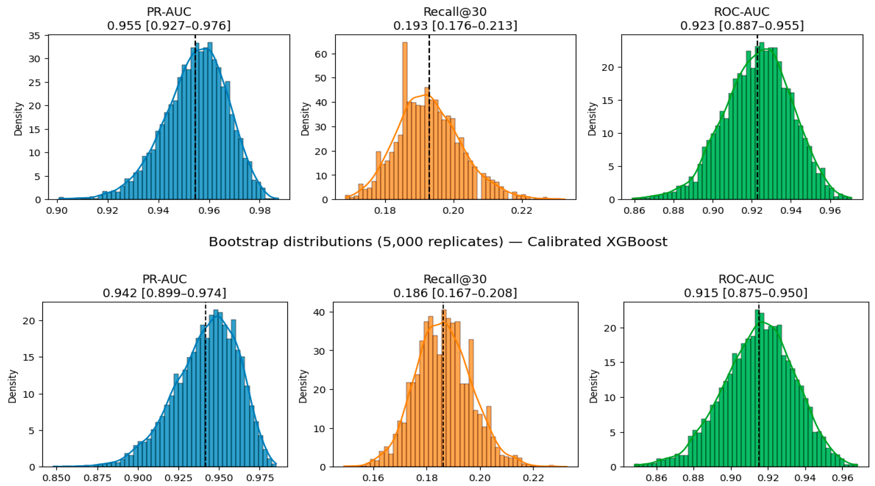
In addition to point estimates, statistical uncertainty was quantified around model performance for the random forest and XGBoost specifications. Uncertainty was assessed using a non-parametric bootstrap applied to the out-of-time test-year evaluation sample. Using the fixed test set predictions from each fitted model, 5000 bootstrap replicates were generated by sampling municipality-year observations with replacement from the test set and recomputing PR-AUC, ROC-AUC, and recall@30 for each replicate. Empirical percentile-based 95% confidence intervals were obtained from the resulting bootstrap distributions. Models were not refitted within bootstrap replicates. Therefore, the bootstrap captured sampling variability in the finite out-of-sample evaluation set rather than refitting uncertainty. The bootstrap distributions for the random forest and XGBoost are reported in Appendix C (Figure A1), while Appendix C,

Table A5. Bootstrap uncertainty summary for out-of-time test performance (2022/23) metrics for random forest and XGBoost. Reported as a point estimate with 95% percentile bootstrap intervals.

Metric	Random Forest	XGBoost
	Estimate (95% CI)	Estimate (95% CI)
PR-AUC	0.955 [0.927–0.976]	0.942 [0.899–0.974]
Recall@30	0.193 [0.176–0.213]	0.186 [0.167–0.208]
ROC-AUC	0.923 [0.887–0.955]	0.915 [0.875–0.950]

summarises the corresponding 95% percentile intervals.

3.7.4. Model Interpretability

Interpretability was addressed by reporting odds ratios from a post-Lasso refit logit model and SHAP-based explanations for the XGBoost model. SHAP focused on XGBoost to provide a single, coherent explanation framework for non-linear effects and to limit redundancy across ensemble explainers. This technique enables the identification of the strongest predictors of higher one-year-ahead distress risk [58]. For the tree-based models, SHapley Additive ExPlanations (SHAP) values were computed using the TreeSHAP algorithm, providing consistent, locally accurate feature attributions for ensemble trees [59]. Meanwhile, with XGBoost, SHAP values were computed using the TreeSHAP approach implemented in SHAP. TreeExplainer provides locally additive feature attributions for tree ensembles [59].

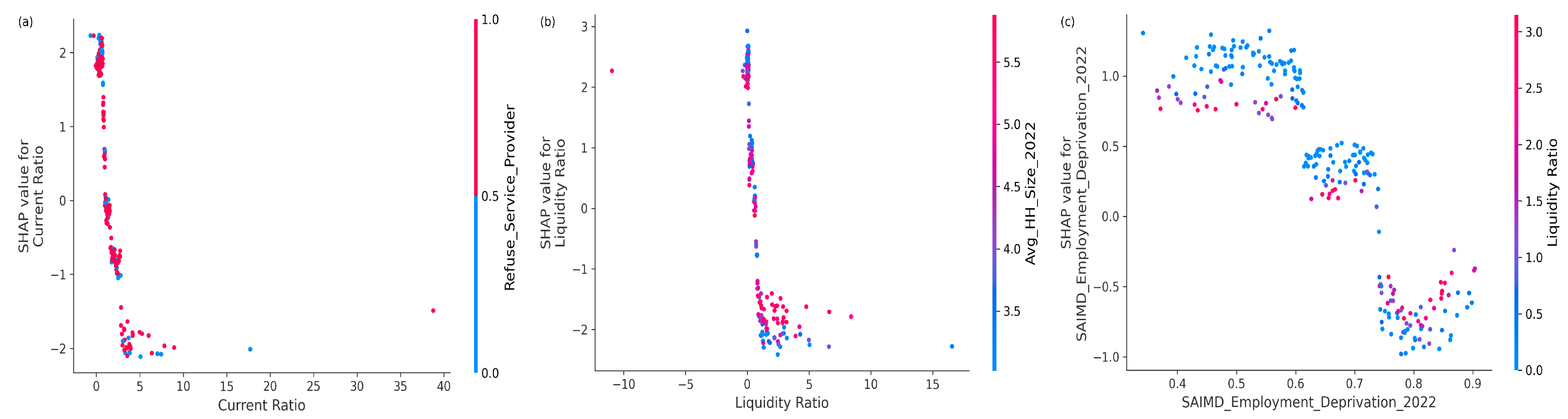
For the held-out 2022/23 test year, SHAP values were computed for each municipality-year, and each predictor and global importance were summarised using the mean absolute SHAP value across test observations. The distribution of SHAP values was visualised for the most influential predictors using a beeswarm (summary) plot [58]. SHAP dependence plots were produced for the most influential predictors to illustrate non-linear effects. This step demonstrated how variation in each predictor is linked with changes in the predicted probability of financial distress conditional on other features.

3.8. Data and Code Availability

All analyses were conducted in Python 3.12.12 (Google Colab) using scikit-learn 1.6.1, pandas 2.2.2, NumPy 2.0.2, XGBoost 3.1.2, and SHAP 0.50.0. The replication package, including scripts for data preparation, the final municipality-year panel, the modelling pipeline, and the Jupyter notebooks that reproduce all tables and figures, is archived in a Zenodo repository. The repository README provides brief run instructions and links for execution via Google Colab.

4. Results

This section provides a concise, precise description of the experimental results, their interpretation, the experimental conclusions, and the empirical results. Descriptive statistics summarise the distribution of financial distress and key indicators across South African municipalities. The predictive performance of the three model classes was reported, followed by an analysis of the most influential predictors and a set of robustness checks on alternative preprocessing choices.

4.1. Descriptive Statistics

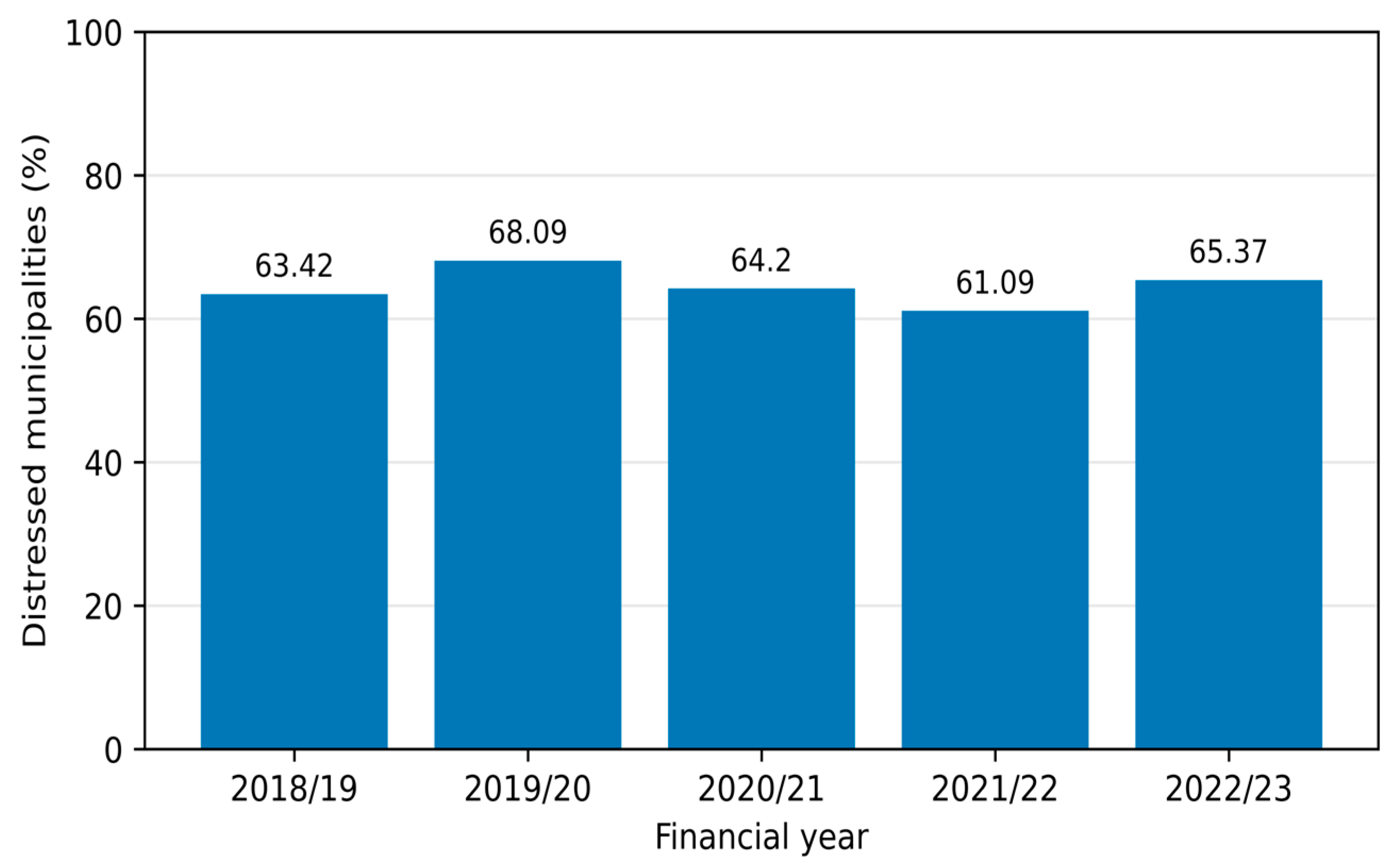
The final dataset comprised 1285 municipality-year observations from 257 South African municipalities between 2018/19 and 2022/23. Based on the official SoLG financial distress flag in Section 3.3, 828 observations (64.4%) were classified as financially distressed and 457 observations (35.6%) as non-distressed. The share of municipalities in distress fluctuated between approximately 61 and 68% over five years, with a local peak in 2019/20. This finding indicated persistent, system-wide fiscal stress rather than a rare or short-lived phenomenon (see Figure 2).

Table 2. Descriptive statistics for selected predictors by distress status.

Variable	Full Sample		Non-Distressed		Distressed		Diff	p-Value
	Mean	Std Dev	Mean	Std Dev	Mean	Std Dev
Cash Coverage (Months)	3.687	21.949	6.796	8.739	1.971	26.41	−4.824	***
Debtors Days	−654.012	34,311.868	−2271.676	57,529.764	238.830	845.74	+2510.505
Operating Expenditure/Revenue	1.000	6.522	0.621	10.916	1.209	0.460	+0.588	***
Grant Share of Operating Revenue	0.478	0.271	0.530	0.302	0.449	0.249	−0.080	***
Employment Deprivation Index	0.644	0.133	0.664	0.151	0.633	0.121	−0.031	***
Education Deprivation Index	0.183	0.053	0.188	0.054	0.181	0.052	−0.007	**
Living Environment Deprivation Index	0.401	0.252	0.472	0.275	0.363	0.229	−0.109	***
Provincial Real GDP-R Growth (%)	0.494	3.555	0.632	3.595	0.418	3.532	−0.214	**
Provincial Unemployment Rate (%)	30.707	6.596	30.299	7.362	30.933	6.125	+0.633	**
CPI Inflation (%)	4.920	1.309	4.945	1.293	4.906	1.318	−0.039
N (Municipality-Years)	1285		457		828

Note: Mean (standard deviation). Diff = distressed—non-distressed. ** and *** denote significance at the 10, 5, and 1 per cent levels, respectively, based on two-sided Wilcoxon rank-sum (Mann–Whitney U) tests and are intended as descriptive contrasts rather than a basis for variable selection. CPI is national-level (varies by year, not municipality); therefore, any group difference reflects year composition rather than cross-sectional variation within a year.

presents descriptive statistics for selected predictors by distress status (mean and standard deviation). These predictors were chosen a priori to provide a concise snapshot of the main variables in the modelling framework. Selection prioritised interpretable indicators for oversight practice in line with the SoLG/NT-13 monitoring logic, consistently available across the 2018/19–2022/23 panel. The complete predictor set, definitions, formulas, and sources are provided in Appendix A, Table A1.

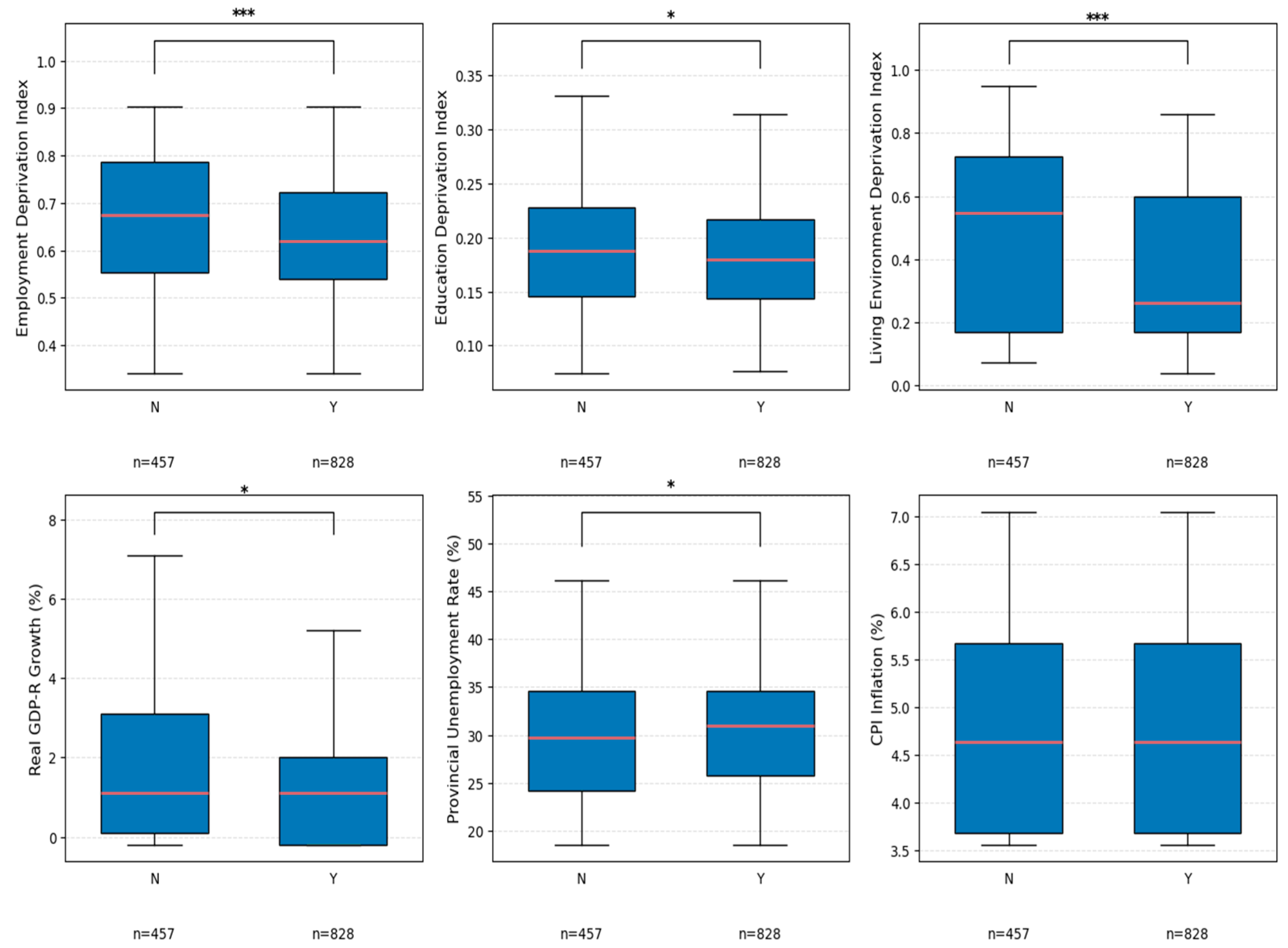
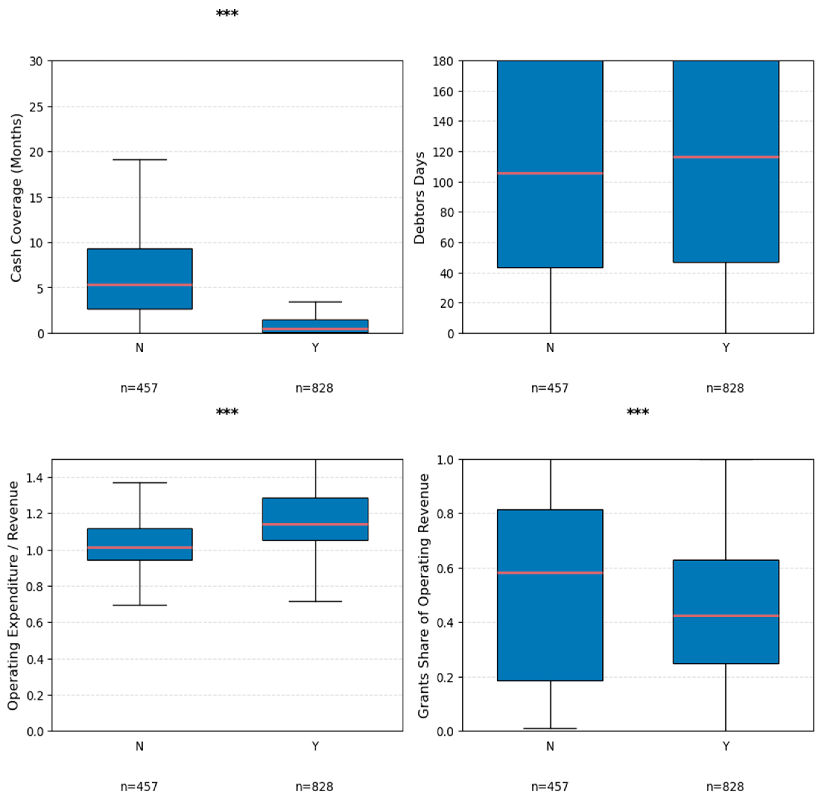
Figure 3 and Figure 4 present the complete distributions of the selected indicators for distressed and non-distressed municipality-years, respectively, using boxplots (sample sizes are displayed below each panel). Given that several indicators exhibit strong skewness and outliers, group variations were assessed using two-sided Wilcoxon rank-sum tests with *, **, and *** denoting significance at the 10, 5, and 1 per cent levels, respectively. The boxes depict the interquartile range with the median, with whiskers extending to 1.5 × IQR.

4.1.1. Financial Indicators

On average, distressed municipalities retain substantially lower cash buffers than non-distressed ones. The mean cash coverage was 1.97 months for distressed municipalities compared with 6.80 months for non-distressed municipalities. This discrepancy is statistically significant at the 1 per cent level (see Table 2). Figure 3 illustrates that the distribution of cash coverage is shifted downwards for distressed municipalities, with a lower median and a shorter upper whisker. This finding suggested that few distressed municipalities sustained high-liquidity buffers.

The operating expenditure-to-revenue ratio was higher for distressed municipalities (mean = 1.21) than for non-distressed municipalities (0.62). The results signalled that distressed municipalities tend to spend more than their realised operating revenue. The boxplots in Figure 3 indicate that this contrast is not driven solely by a small number of extreme observations. The median ratio exceeds one for distressed municipalities and is less than one for non-distressed municipalities, with the difference significant at the 1 per cent level.

Grants constitute a smaller share of operating revenue in distressed municipalities (mean = 0.45) relative to non-distressed municipalities (0.53). The distributions in Figure 3 indicate dispersion in both groups, with a higher median and upper quartile for non-distressed municipalities. This pattern aligns with compositional differences across municipal types: urban municipalities have lower operating grant shares and rely more on own-revenue financing. Nonetheless, fiscal stress occurs through collection, cost, or liability pressures.

Although debtor days exhibit substantial dispersion in both groups, the variation in means between distressed and non-distressed municipalities is not statistically significant (see Table 2). Additionally, the boxplots in Figure 3 exhibit long upper whiskers and several extreme values in both groups. Hence, debtor performance as measured by this indicator is highly variable and potentially unstable in the raw data, with limited evidence of systematic differences by distress status.

4.1.2. Socio-Economic and Macro-Economic Context

The socio-economic context differs systematically across groups. Non-distressed municipalities are generally located in areas with higher employment, education, and living environment deprivation as measured by the SAIMD indices. For example, the mean living environment deprivation index is 0.47 for non-distressed municipalities compared with 0.36 for distressed municipalities. All three deprivation measures revealed statistically significant differences at conventional levels (see Table 2). Figure 4 illustrates that median deprivation scores are consistently higher in non-distressed municipalities, with little overlap in interquartile ranges, particularly for living environment deprivation. This pattern suggests that various non-distressed municipalities are smaller and more rural, whereas a sizeable share of distressed municipalities are larger urban jurisdictions with lower deprivation scores.

At the macro-economic level, distressed municipalities are located in provinces with slightly lower real GDP-R growth (0.42% versus 0.63% for non-distressed municipalities) and higher unemployment rates (30.93% versus 30.30%). The differences are statistically significant at the 5 per cent level. Figure 4 illustrates modest but visible shifts in the distributions. In contrast, the distributions of CPI inflation are nearly identical across the two groups. The difference in means is not statistically significant, as expected considering that CPI is measured at the national level.

These descriptive patterns provide initial evidence that distressed municipalities combine weaker internal financial positions with slightly less favourable provincial macro-economic conditions, and they are also situated in less deprived local socio-economic contexts.

4.2. Model Performance Results

Consistent with Section 3.7.2, the results of PR-AUC for the distressed class are complemented by ROC-AUC and the F1-score for distressed observations, and they are recalled at K = 30.

Table 3. Predictive performance of baseline models on the validation year and out-of-time test year.

Model	PR-AUC (Val)	PR-AUC (Test)	F1 (Val)	F1 (Test)	Recall@30 (Val)	Recall@30 (Test)	ROC-AUC (Test)
Penalised Logistic Regression	0.869	0.934	0.832	0.837	0.189	0.186	0.886
Random Forest	0.967	0.954	0.912	0.881	0.210	0.192	0.923
XGBoost	0.959	0.941	0.877	0.886	0.210	0.186	0.915

Note: PR-AUC is reported for the distressed class. Threshold-based classification metrics (F1) use a fixed probability threshold of 0.5. Recall@30 is a top-K early-warning metric with K = 30 (≈12% of municipalities per year). ROC-AUC is reported for the 2022/23 out-of-time test year.

demonstrates the predictive performance of the three baseline models on the validation year (2021/22) and on the out-of-time test year (2022/23). Appendix C, Figure A1 lists the distributions of 95% bootstrap confidence intervals (5000 replicates) for the test-year PR-AUC, recall@30, and ROC-AUC of random forest and XGBoost. Meanwhile, Appendix C, Table A5 summarises the 95% percentile intervals.

On the held-out test year, the penalised logistic regression model yielded a PR-AUC of 0.934 and an ROC-AUC of 0.886, with an F1-score of 0.837 for the distressed class. At the operational cut-off corresponding to the top 30 municipalities, the recall was 0.186, indicating that under one-fifth of distressed municipalities were captured in the prioritised group. The tree-based models improved discrimination metrics. The random forest obtained the highest PR-AUC (0.954) and ROC-AUC (0.923), while XGBoost yielded the highest F1-score (0.886). Across models, recall@30 on the test year remained in a narrow range (0.186–0.192), consistent with substantially high precision in the top-risk group. From an oversight perspective, prioritising approximately 30 municipalities for closer monitoring would focus on those currently in or nearing financial distress, with few false positives.

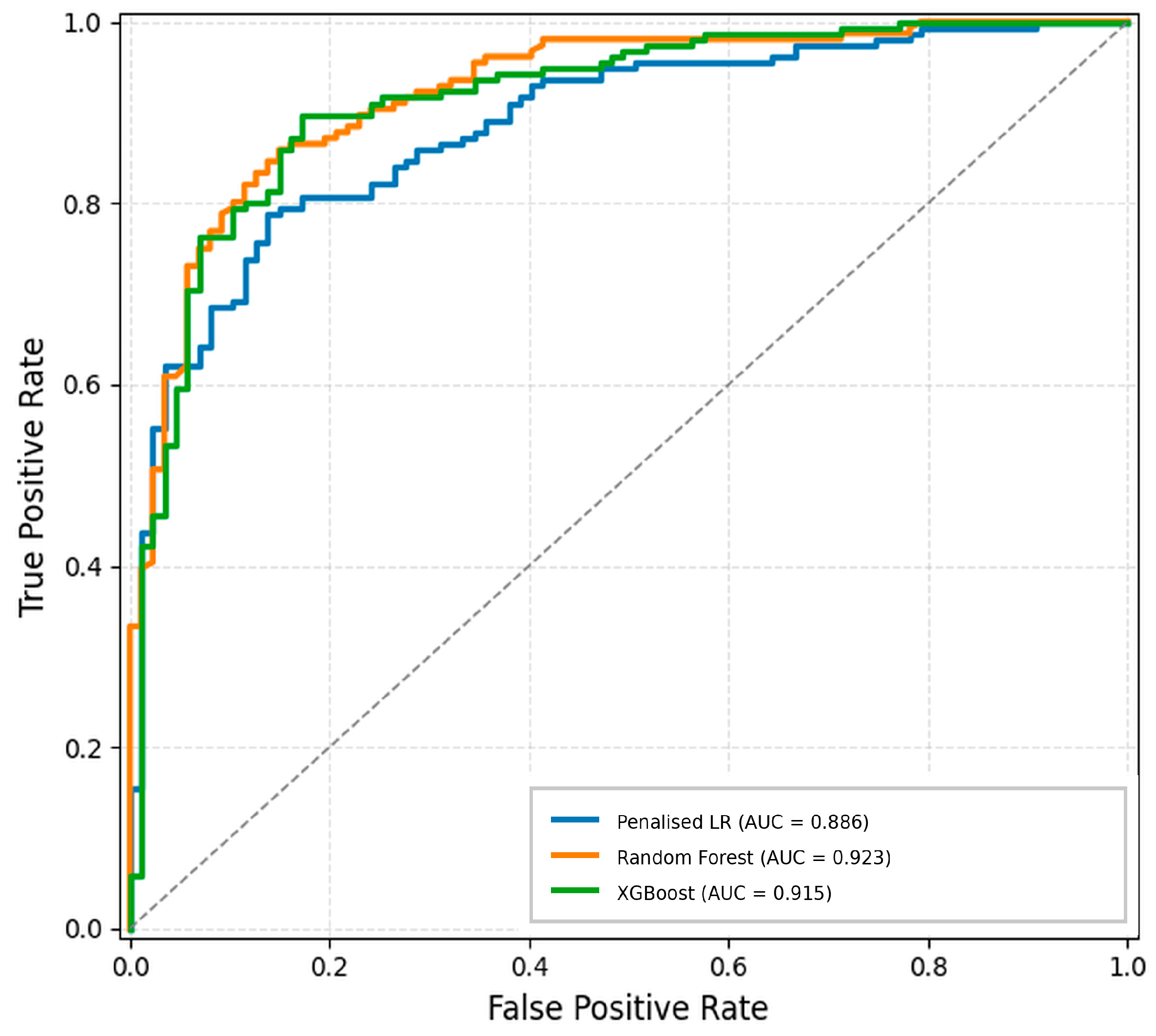
Figure 5 presents the ROC curves for the penalised logistic regression, random forest, and XGBoost models on the 2022/23 test set.

All models achieved strong discrimination, with ROC-AUC values of 0.886 for the penalised logistic regression, 0.923 for the random forest, and 0.915 for XGBoost. The curves confirmed the ranking suggested by the PR-AUC leaderboard. Both tree ensembles outperformed the logistic baseline in classification performance, with the random forest achieving the highest ROC-AUC. Given the high prevalence of distress, the current study focused primarily on PR-AUC and top-K metrics in the main discussion. Nonetheless, the ROC curves provided a familiar benchmark, denoting that the models separate distressed and non-distressed municipalities well across a broad range of thresholds.

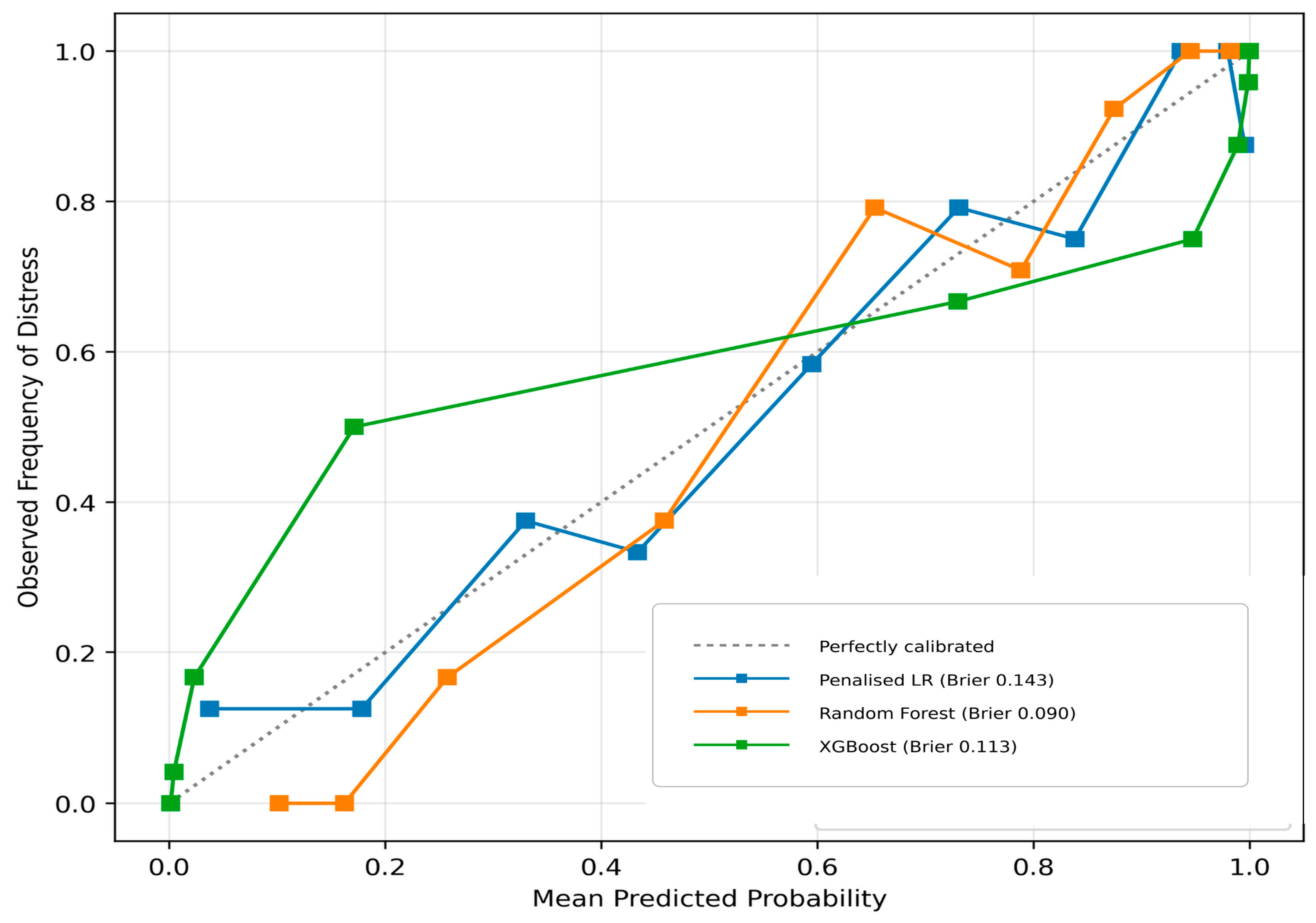
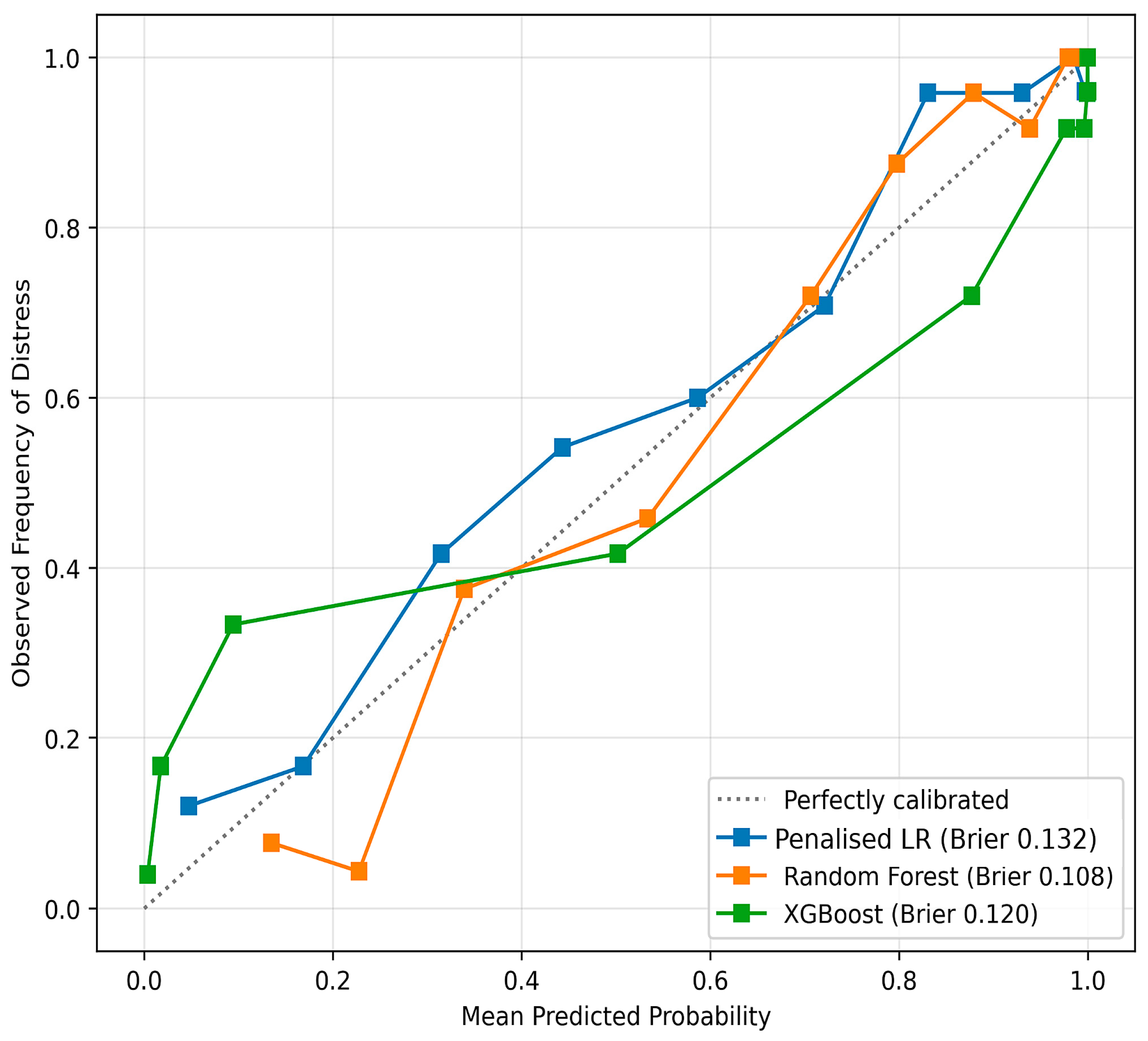
Calibration diagnostics indicated that the probabilistic forecasts were well aligned with observed distress frequencies. The dotted line represents perfect calibration. All three models lie close to this line across most of the probability range, with only moderate deviations at the lowest and highest predicted probabilities. Random forest is slightly closer to the diagonal than the other models, particularly in the 0.4–0.8 range. Meanwhile, logistic regression depicts mild overprediction in the middle bins, and XGBoost slightly underpredicts distress at lower scores. Figure 6 demonstrates reliability curves for the three models on the out-of-time test year (2022/23), with mean predicted probabilities on the horizontal axis and observed distress rates in each decile on the vertical axis. Appendix C, Figure A2 presents the validation-year calibration.

Table 4. Brier scores on validation and test sets.

Model	Set	Brier Score
Logistic Regression	Validation	0.143
Logistic Regression	Test	0.132
Random Forest	Validation	0.090
Random Forest	Test	0.108
XGBoost	Validation	0.113
XGBoost	Test	0.120

presents the Brier scores on the validation year (2021/22) and out-of-time test year (2022/23), with lower values indicating better calibration.

These visual impressions are consistent with the Brier scores. In the validation year (2021/22), the Brier score equals 0.143 for logistic regression, 0.090 for random forest, and 0.113 for XGBoost compared with a naïve baseline of approximately 0.23 obtained by predicting the unconditional distress rate for all observations. In the test year, the Brier scores improved to 0.132 for logistic regression, 0.108 for random forest, and 0.120 for XGBoost. Thus, all three models produced substantially better probability forecasts than the naïve benchmark. The random forest performed best, followed closely by XGBoost and logistic regression. Collectively, the PR-AUC and recall-at-30 results indicate that the calibration analysis reveals that the models rank municipalities by risk and provide numerically meaningful probabilities that can support risk-based oversight and scenario analysis.

Realistic oversight capacity was reflected by examining a threshold that flags the 30 municipalities with the highest predicted risk in the 2022/23 test year, corresponding to approximately 12.3% of all municipalities in the sample.

Table 5. Top-30 early-warning performance on the 2022/23 test year.

Model	TP	FP	FN	Precision@K	Recall@K	Workload (%)
Penalised Logistic Regression	29	1	127	0.967	0.186	12.3
Random Forest	30	0	126	1.000	0.192	12.3
XGBoost	29	1	127	0.967	0.186	12.3
Naïve (Last Year)	27	3	129	0.900	0.173	12.3

Notes: K = 30 (12.3% workload). Precision@K = TP/K and recall@K = TP/(TP + FN) computed on the 2022/23 test year.

demonstrates the top-K early-warning performance on the 2022/23 test year (K = 30), including true positives, false positives, false negatives, and workload share.

For the random forest model, all 30 flagged municipalities were distressed (TP = 30, FP = 0), yielding a precision@30 of 1.000 and a recall@30 of 0.192. Thus, the high-risk portfolio contains no false alarms but captured only approximtely 19% of all distressed municipalities (FN = 126). The penalised logistic regression and XGBoost models displayed a similar trade-off. Both flag 29 distressed municipalities and one non-distressed municipality (TP = 29, FP = 1), yielding a precision@30 of 0.967 and a recall@30 of 0.186 (FN = 127). As for benchmarking under a policy-relevant workload constraint, all models were compared against a naïve “last-year distress” rule using the Top-30 early-warning evaluation. A monitoring programme that focuses intensive support on 30 municipalities would allocate nearly all efforts to genuinely distressed municipalities, albeit overlooking most distressed cases that fall under the Top-30 cut-off. In practice, false negatives are most likely to occur where a municipality’s position deteriorates sharply between the lagged predictor year (t − 1) and the outcome year (t) or where distress is driven by idiosyncratic events that are imperfectly captured by routine ratios (for instance, governance shocks, litigation, or sudden revenue shortfalls). To mitigate this risk, a two-tier deployment is recommended: (i) an intensive support portfolio (Top-30) and (ii) a broader watch list, such as Top-60 or Top-90, for lighter touch monitoring and rapid reassessment as new in-year information becomes available.

Sensitivity to operational thresholds is conceptually straightforward. As K increases, recall@K rises mechanically because more municipalities are flagged, while precision@K typically declines as the portfolio extends beyond the highest-risk tail. Similarly, moving a fixed probability threshold below 0.5 increases sensitivity at the expense of more false positives, while higher thresholds do the reverse. For this reason, we emphasise threshold-free discrimination (PR-AUC/ROC-AUC) and calibration and interpret top-K performance as a capacity-linked operating point rather than a unique optimum.

From an oversight perspective, these results indicate that the models are effective at concentrating attention on the worst-off municipalities (high precision). Nevertheless, additional tiers of support or a larger K value are needed if the policy objective is to detect a larger share of distressed municipalities, considering that the cost of a false negative (failing to identify a distressed municipality) tends to exceed the cost of a false positive (providing additional scrutiny to a municipality that becomes financially sound). These findings support the use of generous thresholds when monitoring resources permit or complementing the Top-30 portfolio with a secondary “watch list” based on slightly lower predicted probabilities.

4.3. Drivers of Financial Distress

This section presents the analysis results based on the methods in Section 3.7.4. The odds ratios from a post-Lasso logistic regression refit were discussed (used to provide coefficient-based effect estimates for key predictors), followed by SHAP-based variable importance and partial-dependence patterns from the tree-based models. This method enables identifying the indicators most consistently associated with a higher predicted risk of financial distress.

Table 6. Odds ratios from post-Lasso logistic regression of municipal financial distress on lagged, standardised predictors (training sample: 2019/20–2020/21).

Feature	Odds Ratio	95% CI Lower	95% CI Upper	p-Value
Total_OpEx_per_capita	307.581	17.886	5289.378	<0.001
Own_Revenue_per_capita	0.013	0.001	0.129	<0.001
Creditor days	9.883	1.416	69.006	0.021
Net asset ratio	0.155	0.035	0.692	0.015
Cash plus investments	0.281	0.096	0.819	0.020
Cash or cash equivalent position less applications	0.301	0.038	2.376	0.255
Pop. density per km2	3.113	1.009	9.602	0.048
Unauth_to_OpEx	2.687	1.225	5.897	0.014
Operating_Surplus_Abs_Audited	2.419	0.696	8.411	0.165
GF_Size	0.464	0.156	1.381	0.168
UIFW_Total	1.992	0.552	7.195	0.293
SAIMD_LivingEnv_Deprivation_2022	0.513	0.236	1.116	0.092
Grants_per_capita	0.522	0.265	1.030	0.061
Median_Age_2022	0.573	0.319	1.028	0.062
GF_to_Revenue	0.593	0.045	7.828	0.691
Current ratio	0.600	0.368	0.976	0.040
UIFW_to_OpEx	1.606	0.034	76.514	0.810
Cash coverage (months)	0.634	0.388	1.036	0.069
GF_to_OpEx	1.453	0.383	5.519	0.583
Electricity_Service_Provider	1.449	0.854	2.459	0.169

Notes: Predictors are lagged by one year and standardised; odds ratios, therefore, reflect a one SD increase in continuous predictors (or presence versus absence for binary predictors). Confidence intervals are Wald-type 95% intervals computed using municipality-clustered robust standard errors and are exponentiated to the odds ratio scale. p-values < 0.001 are reported as “<0.001”.

reports odds ratios from the post-Lasso logistic regression refit predicting one-year-ahead municipal financial distress using lagged, standardised predictors (training period: 2019/20–2020/21). The estimates reported 95% confidence intervals based on municipality-clustered robust standard errors. Because predictors are standardised, odds ratios reflect a one standard deviation change. In the cases of heavy-tailed expenditure-intensity variables, the exponentiation can yield very large odds ratios; therefore, their direction and statistical support are more informative than the headline magnitude.

The results highlighted a clear and policy-relevant set of early-warning signals. The strongest protective factor is own-revenue generation per capita: a one standard deviation increase in own revenue per resident is associated with 98.7% lower odds of distress in the following year (OR = 0.013, p < 0.001). Conversely, municipalities with one standard deviation higher total operating expenditure per capita have over 300 times higher odds of distress (OR = 307.6, p < 0.001). The results reflect severe cost pressures in strained local governments.

Liquidity and solvency remain critical. A one standard deviation improvement in the net asset ratio reduces the odds of distress by approximately 84% (OR = 0.155, p = 0.015). In contrast, higher cash holdings and a higher current ratio are strongly protective (OR = 0.28 and 0.60, respectively). Longer creditor payment periods (creditor days) substantially increased the risk of formal distress (OR = 9.88, p = 0.021), consistent with cash-flow difficulties and supplier pressure as precursors of formal distress.

Governance and expenditure control variables are crucial. Higher levels of unauthorised, irregular, fruitless, and wasteful (UIFW) expenditure relative to operating expenditure are linked with 2.7 times higher odds of distress (OR = 2.69, p = 0.014). Greater population density and reliance on capital grants show more modest but still significant associations.

Taken together, these findings confirm that municipal financial distress in South Africa is driven primarily by poor own-revenue capacity, excessive operating cost burdens, liquidity shortfalls, and poor expenditure discipline. These factors are observable at least one full fiscal year before formal distress declarations.

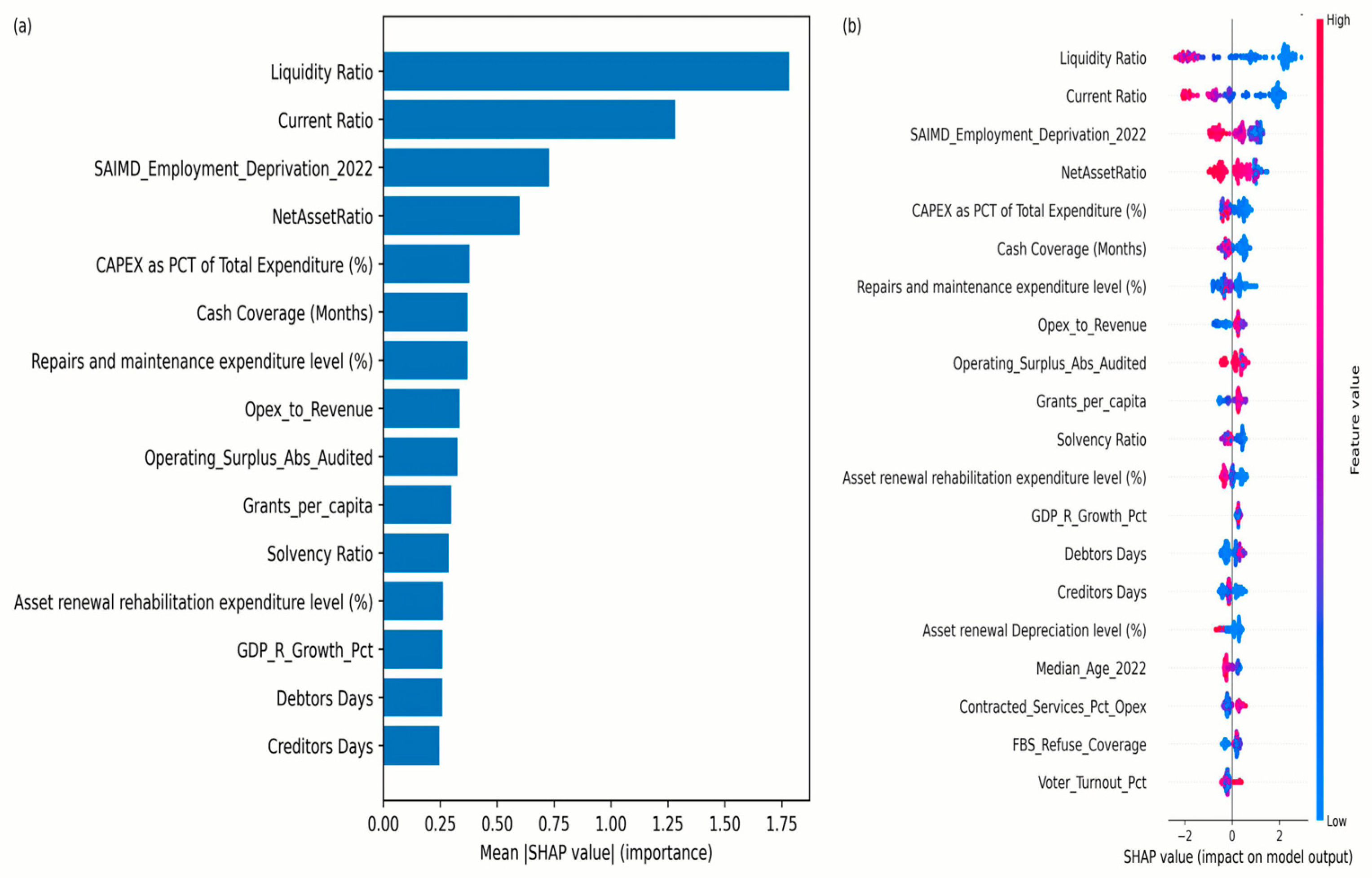
Apart from interpreting the signs and magnitudes of the penalised logistic regression coefficients, SHAP values were applied to the XGBoost model to represent a non-linear ensemble and assess variable importance and non-linear effects. The tree-based models (random forest and XGBoost) yield similar rankings of the most influential predictors. Hence, for parsimony, the SHAP results were reported only for the XGBoost. The SHAP summary plot for the 2022/23 test year (see Figure 7) indicates that liquidity and solvency indicators are the dominant drivers of predicted financial distress.

Low values of the liquidity ratio and current ratio (blue points on the right of the plot) are connected with large positive SHAP values. This situation drives the predicted probability towards distress, whereas higher liquidity and current ratios (red points on the left) reduce the predicted risk. Net asset ratios and cash coverage months also exhibit protective effects, with higher values shifting SHAP values towards lower predicted distress. This situation reinforces the significance of cash and balance sheet solvency within the extended framework.

SHAP dependence plots for the liquidity ratio, current ratio, and employment deprivation (reported in Appendix C, Figure A3) corroborate these patterns and demonstrate that the predicted probability of distress rises sharply as liquidity and current ratios fall below their medians.

Differences in the selection of important features between the post-Lasso and tree-based SHAP are expected. The post-Lasso enforces sparsity and, under correlated predictors, often selects one representative variable from a cluster, while tree-based SHAP can distribute importance across correlated features and capture interaction and non-linear threshold effects. Accordingly, consistency in the core signals across methods is more informative than one-to-one overlap in selected predictors.

Across the two explanatory lenses, a coherent intersection emerges. Liquidity and balance sheet strength (liquidity ratio, current ratio, net asset ratio, and cash coverage) are consistently protective, while cost pressure and weak expenditure control (operating expenditure intensity, creditor payment delays, and UIFW-related indicators) elevate one-year-ahead distress risk. This convergence strengthens confidence that the identified drivers are not artefacts of a single interpretability method and supports their use as policy-relevant early-warning signals.

4.4. Robustness Checks

4.4.1. Agreement Between Reconstructed NT-13 Labels and Official SoLG Classification

The primary outcome in this study is the official SoLG financial distress flag in the National Treasury. To verify that the reconstructed NT-13 rule set is consistent with this classification, the reconstructed NT-13 labels were compared to the official SoLG flag for all 1285 municipality-year observations.

Table 7. Confusion matrices comparing the official SoLG financial distress flag with reconstructed NT-13 labels.

Official SoLG Flag	Reconstructed Broad NT-13 Label			Reconstructed Strict NT-13 Label
	0 (Non-Distressed)	1 (Distressed)	Total	0 (Non-Distressed)	1 (Distressed)	Total
0 (non-distressed)	423	34	457	440	17	457
1 (distressed)	41	787	828	237	591	828
Total	464	821	1285	677	608	1285

reports the resulting confusion matrices for the reconstructed broad and strict NT-13 labels.

Under the broad label reconstruction, the two classifications coincide in 1210 cases. A total of 423 municipality-years were classified as non-distressed and 787 as distressed by both approaches. Disagreements were limited to 34 observations flagged as distressed by the reconstructed broad label but not by SoLG. Additionally, 41 observations were flagged as distressed by SoLG but not by the reconstructed label. Distress prevalence is also similar under the two approaches (0.644 for the official SoLG flag and 0.639 for the reconstructed broad label).

Table 8. Agreement statistics and prevalence under alternative distress definitions (n = 1285).

Comparison	Accuracy	Precision	Recall	F1-score	Prevalence: SoLG Distressed	Prevalence: Broad Distressed	Prevalence: Strict Distressed
SoLG vs. Broad (NT-13)	0.942	0.959	0.950	0.955	0.644	0.639	0.473
SoLG vs. Strict (NT-13)	0.802	0.972	0.714	0.823	0.644	0.639	0.473

Note: Agreement statistics treat the official SoLG flag as the reference classification (positive = distressed).

summarises the agreement statistics for the alternative definitions.

4.4.2. Sensitivity to a Stricter Distress Definition

The present study examined whether the findings respond to a more stringent definition of financial distress. A strict distress label was constructed based on Section 3.3 to record more severe cases. Under the strict definition, a municipality-year is classified as distressed only if fewer than seven of the 13 indicators are within norm and at least one of the current ratio or solvency ratio is below one. The strict label constitutes a subset of the broader distress cases and has a lower prevalence, concentrating on more acute instances of financial stress. As all predictors lagged by one year, the strict label at year t is predicted using information available at t − 1.

Table 8 presents agreement statistics and prevalence under alternative distress definitions, comparing the official SoLG financial distress flag to the reconstructed broad and strict NT-13 labels. The table reports accuracy, precision, recall, and the F1-score for the distressed class for both comparisons (SoLG vs. Broad and SoLG vs. Strict). Distress prevalence was also listed under the official SoLG flag and under the broad and strict NT-13 definitions.

Table 8 indicates that the strict definition reduces the prevalence of distress to 0.473, compared with 0.644 under the official SoLG flag and 0.639 under the reconstructed broad label. The findings align with the identification of a narrower set of more severe cases.

The penalised logistic regression, random forest, and XGBoost models were re-estimated using the strict label as the outcome while keeping the predictor set and modelling pipeline constant. The strict label performance results are exhibited in Appendix C,

Table A4. Strict label predictive performance on validation and held-out test years.

Model	PR-AUC (Val)	PR-AUC (Test)	F1 (Val)	F1 (Test)	Recall@30 (Val)	Recall@30 (Test)	ROC-AUC (Test)
Penalised logistic regression	0.849	0.856	0.177	0.671	0.234	0.256	0.850
Random forest	0.911	0.895	0.809	0.8174	0.226	0.256	0.912
XGBoost	0.908	0.891	0.795	0.7768	0.242	0.256	0.903

Note: Under the strict label, the number of distressed municipalities is 124 in 2021/22 and 117 in 2022/23; hence, the maximum achievable recall@30 is 30/124 = 0.242 (Val) and 30/117 = 0.256 (test).

(held-out 2022/23 test year). The random forest model performed best overall under the strict definition (PR-AUC 0.895; ROC-AUC 0.912; F1 0.817), followed by the XGBoost model (PR-AUC 0.891; ROC-AUC 0.903; F1 0.777). Meanwhile, the penalised logistic regression model remained competitive (PR-AUC 0.856; ROC-AUC 0.850; F1 0.671). For the Top-30 early-warning portfolio, all three models achieved precision@30 = 1.0000 and recall@30 = 0.256, which equals the theoretical maximum given the 117 distressed municipalities under the strict definition in 2022/23 (30/117 = 0.256).

The model ranking and the early-warning conclusions remained stable under a more stringent distress definition, demonstrating that the main findings are not an artefact of the baseline outcome construction.

5. Discussion and Conclusions

5.1. Overview of Main Findings

The present study aimed to develop and evaluate models that predict one-year-ahead municipal financial distress in South Africa using routinely collected financial, governance, and contextual indicators within a time-aware modelling framework designed to reduce temporal leakage. This objective was achieved by combining a strictly time-ordered training, validation and testing split, lagged predictors, and calibration [17]. The results disclosed that municipal distress is not random, with out-of-time PR-AUC values of 0.934–0.954 and ROC-AUC values of 0.886–0.923 on the 2022/23 test year. Even a transparent penalised logistic regression model yielded a high PR-AUC and good discrimination on an out-of-time test year. Furthermore, the random forest and XGBoost models produced modest but consistent results in PR-AUC, F1-score, and probability calibration. These findings align with earlier municipal FDP studies, which discovered that tree-based ensemble models add predictive value to local government data [13,16]. Under a policy-relevant Top-30 rule (12.3% workload), all models achieved high precision on the 2022/23 test year (0.967–1.000), with the random forest identifying 30 of 30 distressed municipalities (precision@30 = 1.000; recall@30 = 0.192) compared with the naïve last-year rule (precision@30 = 0.900; recall@30 = 0.173).

Interpretability analysis using both odds ratios and SHAP values disclosed a stable structure in the predictors of distress, enabling transparent explanations for tree-based models [21]. Liquidity ratios, current ratios, and cash holdings emerged as the strongest protective factors. In contrast, high operating expenditure per capita, poor operating results, and long creditor payment periods are linked to substantially higher distress risk. Governance-related indicators, specifically unauthorised expenditure relative to operating expenditure, further distinguish distressed from non-distressed municipalities. Additionally, socio-economic and deprivation indices exerted smaller but meaningful effects after controlling for financial performance. Notably, some governance and political structure variables included in the full predictor set added a limited incremental signal in the study panel once financial ratios were accounted for and, therefore, do not appear among the most influential drivers in the main interpretability outputs.

5.2. Implications for the Kooij Framework and Its Extension

The findings validate the core dimensions in [22]’s municipal financial health conceptual framework. Cash and liquidity ratios, current liabilities coverage, and solvency ratios were the most influential predictors and displayed the expected signs. Long-term solvency and fiscal structure were reflected in the strong negative relationship between net asset ratios and distress and in the protective effect of higher own revenue per capita. Service-level solvency was noted and assessed using expenditure intensity and free basic services coverage. Nonetheless, the models indicated that the composition and efficiency of operating expenditure are at least as important as the sheer level of service demand.

The results confirmed the need to include institutional and contextual factors applicable in developing country municipalities [39,40]. Governance quality, as reflected in unauthorised expenditure and related audit findings, significantly contributes to the prediction of distress, even after accounting for cash and solvency indicators. This condition proves that institutional weaknesses and failures of budget discipline are crucial to comprehending local fiscal crises [30,40]. Socio-economic context, captured by employment deprivation and population density, moderately influences distress risk. This effect suggests that municipalities in more disadvantaged or complex environments are structurally more vulnerable, specifically when their own revenue bases are weak. The SHAP analysis revealed that these governance and contextual indicators complement rather than replace traditional financial ratios. This finding reinforces the case for an extended, multi-dimensional fiscal health framework tailored to developing countries.

5.3. Policy and Oversight Implications

For public finance practitioners, the results demonstrated that early-warning models based on existing administrative data provide a credible, empirically grounded complement to judgement-based assessments of municipal risk. The high precision in the top-risk group suggests that a small portfolio of municipalities flagged by the models would usually include genuinely distressed cases (precision@30 = 0.967–1.000). This condition provides a practical basis for triaging intensified monitoring, diagnostic support, and escalation planning within existing oversight capacity constraints. This finding is valuable for provincial and national treasuries that experience capacity constraints and must prioritise technical support, intervention planning, and conditional grant monitoring [19,56].

The prominence of cash management and creditor payment behaviour indicators outlines the importance of enforcing basic cash management and payment discipline as first-line safeguards against fiscal distress. Simultaneously, the strong role of own revenue per capita and net asset ratios outlines deeper structural drivers of resilience, such as the breadth of the tax base, the enforceability of billing and collection systems, and the maintenance of infrastructure assets. The significant contribution of unauthorised expenditure ratios indicates that expenditure control failures are systematically associated with distress risk. Nevertheless, addressing symptoms through ex post corrective actions without tackling underlying governance weaknesses is unlikely to resolve distress sustainably.

The findings provided an empirical lens on the existing 13-indicator framework for the National Treasury. Most NT indicators (current ratio, solvency, cash coverage, operating surplus, and debtor and creditor days) emerged as critical predictors, supporting their continued use as the backbone of financial health monitoring. Nonetheless, the models also highlighted the predictive value of additional ratios such as operating expenditure per capita, repairs and maintenance effort, and unauthorised expenditure to operating expenditure. These results inform future refinements of the NT framework by distinguishing a smaller set of core early-warning indicators from supplementary diagnostic ratios and by explicitly integrating governance and socio-economic variables into risk assessments.

Transferability of the design of this study to other oversight regimes depends on separating portable design choices from South Africa-specific inputs. The portable elements include the leakage-aware time-ordered evaluation, class imbalance handling via weighting, calibration assessment, and the capacity-constrained top-K decision rule that converts scores into actionable monitoring lists. Context-specific elements include the distress label (SoLG/NT-13 rule structure), the precise indicator definitions and thresholds, and the institutional escalation mechanisms embedded in MFMA-aligned oversight practice. In other countries, the workflow can be replicated by substituting locally valid distress triggers and fiscal indicators while retaining the same time-aware modelling, calibration, and capacity-linked decision design.

5.4. Limitations and Directions for Future Research

Several limitations were identified. First, the analysis covered a short period, with four usable outcome years after lagging predictors. The short panel also constrains the ability to assess robustness to structural breaks or changes in reporting practices. The out-of-time test year (2022/23) remains within the same institutional and reporting framework (NT-13, MFMA-aligned oversight and mSCOA-based reporting). Therefore, the evidence supports short-horizon forward-looking use rather than performance under major accounting reforms or abrupt institutional regime shifts. This situation limits the ability to study longer-term dynamics and to evaluate model performance across various macro-fiscal regimes.

Second, although the distress definition closely mirrors National Treasury logic, the term remains a constructed proxy that combines the composite score and solvency overrides. Relatedly, the SoLG flag is an administrative classification that may embed expert judgement. The reconstructed NT-13 labels provide a sensitivity check to alternative rule-based definitions. Meanwhile, alternative definitions, such as those based on actual payment defaults or intervention events, could yield varying patterns and require further investigation.

Third, the study incorporated a diverse set of financial, governance, and socio-economic indicators. Nonetheless, significant dimensions remain imperfectly measured. Specifically, the environmental and disaster risk indicators proposed in the extended framework could not be included due to data availability. Future works are suggested to incorporate municipal-level hazard and vulnerability indices once the CSIR Green Book data becomes accessible. Similarly, the models only implicitly consider policy and institutional changes over time. Incorporating specific indicators of reform efforts, political turnover, and changes in intergovernmental grant rules could increase understanding of the ways institutional dynamics interact with financial distress.

Although the random forest and XGBoost models yielded stronger predictive performance than logistic regression, they remain black box models to numerous practitioners. The use of SHAP values and partial-dependence plots in the current study mitigates this concern. Nevertheless, deeper investigation is needed to translate model outputs into actionable, user-friendly tools for treasuries and municipalities, including dashboards, scenario analysis, and integration with existing early-warning processes.

The study demonstrated that a parsimonious set of financial and governance indicators can generate accurate, well-calibrated predictions of municipal financial distress in a developing country setting. By integrating these predictors with an extended solvency framework and in a time-aware modelling design, the analysis provides methodological and practical contributions to the literature on local government fiscal health.

References

1. Glasser, M.D.; Wright, J. South African municipalities in financial distress: What can be done? Law Democr. Dev. 2020, 24, 413–441. [Google Scholar] [CrossRef] [Scilit]
2. National Treasury. The State of Local Government Finances and Financial Management for the Financial Year Ended as at 30 June 2023; National Treasury: Pretoria, South Africa, 2024.
3. Zweni, A.; Koma, S.; Ndevu, Z. Coalition effects on financial and service delivery performance in metropolitan municipalities in Gauteng. J. Local Gov. Res. Innov. 2024, 5, a183. [Google Scholar] [CrossRef] [Scilit]
4. Republic of South Africa (RSA). Municipal Finance Management Act, No. 56 of 2003; Government Printer: Pretoria, South Africa, 2003.
5. Mbulawa, A. Understanding the impact of financial sustainability on South African municipalities. J. Transdiscipl. Res. South. Afr. 2019, 15, a656. [Google Scholar] [CrossRef] [Scilit]
6. Ruplal, K. The Impact of Socioeconomic Factors on Municipal Fiscal Health in South Africa. Doctoral Dissertation, Stellenbosch University, Stellenbosch, South Africa, 2022. [Google Scholar]
7. Shozi, S.R. Audit Outcomes and Financial Health of Municipalities in South Africa. Master’s Thesis, University of Cape Town, Cape Town, South Africa, 2023. [Google Scholar]
8. Lukáč, J.; Teplická, K.; Čulková, K.; Hrehová, D. Evaluation of the financial performance of the municipalities in Slovakia in the context of multidimensional statistics. J. Risk Financ. Manag. 2021, 14, 570. [Google Scholar] [CrossRef] [Scilit]
9. Zhuang, Y.; Wei, H. Early warning model and prevention of regional financial risk integrated into legal system. PLoS ONE 2023, 18, e0286685. [Google Scholar] [CrossRef] [Scilit] [PubMed]
10. Kang, H.; Chen, G. The Effect of Fiscal Stress Labels on Local Governments’ Financial Management: Evidence from New York State Fiscal Stress Monitoring System. Public Financ. Rev. 2024, 52, 643–678. [Google Scholar] [CrossRef] [Scilit]
11. Shiddiqy, R.A.; Prihatiningtias, Y.W. The prediction of financial distress probability in East Java province governments. Int. J. Res. Bus. Soc. Sci. 2022, 11, 152–160. [Google Scholar] [CrossRef] [Scilit]
12. Alaminos, D.; Fernández, S.; García, F.; Fernández, M. Data mining for municipal financial distress prediction. In Advances in Data Mining: Applications and Theoretical Aspects; Perner, P., Ed.; Lecture Notes in Computer Science; Springer: Berlin/Heidelberg, Germany, 2018; Volume 10933, pp. 296–308. [Google Scholar] [CrossRef] [Scilit]
13. Antulov-Fantulin, N.; Lagravinese, R.; Resce, G. Predicting bankruptcy of local government: A machine learning approach. J. Econ. Behav. Organ. 2021, 183, 681–699. [Google Scholar] [CrossRef] [Scilit]
14. Li, X.; Ge, X.; Chen, C. Several explorations on how to construct an early warning system for local government debt risk in China. PLoS ONE 2022, 17, e0263391. [Google Scholar] [CrossRef] [Scilit]
15. Piermarini, D.; Sudoso, A.M.; Piccialli, V. Predicting municipalities in financial distress: A machine learning approach enhanced by domain expertise. arXiv 2023, arXiv:2302.05780. [Google Scholar] [CrossRef] [Scilit]
16. Liu, R.P.; Li, H.; Yoon, K.; Vasarhelyi, M.A. Using Machine Learning Algorithms to Improve Fiscal Distress Prediction Models: The Case of U.S. Local Governments. J. Inf. Syst. 2025, 39, 131–155. [Google Scholar] [CrossRef] [Scilit]
17. Roberts, D.R.; Bahn, V.; Ciuti, S.; Boyce, M.S.; Elith, J.; Guillera-Arroita, G.; Hauenstein, S.; Lahoz-Monfort, J.J.; Schröder, B.; Thuiller, W.; et al. Cross-validation strategies for data with temporal, spatial, hierarchical, or phylogenetic structure. Ecography 2017, 40, 913–929. [Google Scholar] [CrossRef] [Scilit]
18. Hewamalage, H.; Ackermann, K.; Bergmeir, C. Forecast evaluation for data scientists: Common pitfalls and best practices. Data Min. Knowl. Discov. 2022, 37, 788–832. [Google Scholar] [CrossRef] [Scilit]
19. Kleinberg, J.; Ludwig, J.; Mullainathan, S.; Obermeyer, Z. Prediction Policy Problems. Am. Econ. Rev. 2015, 105, 491–495. [Google Scholar] [CrossRef] [Scilit]
20. Hancock, J.; Khoshgoftaar, T.M.; Johnson, J. Evaluating classifier performance with highly imbalanced Big Data. J. Big Data 2023, 10, 42. [Google Scholar] [CrossRef] [Scilit]
21. Lundberg, S.M.; Erion, G.; Chen, H.; DeGrave, A.; Prutkin, J.M.; Nair, B.; Katz, R.; Himmelfarb, J.; Bansal, N.; Lee, S.I. From local explanations to global understanding with explainable AI for trees. Nat. Mach. Intell. 2020, 2, 56–67. [Google Scholar] [CrossRef] [Scilit]
22. Kooij, J.; Groot, T. Towards a comprehensive assessment system of local government fiscal health. Maandbl. Voor Account. En Bedrijfsecon. 2021, 95, 233–244. [Google Scholar] [CrossRef] [Scilit]
23. Zafra-Gómez, J.L.; López-Hernández, A.M.; Hernández-Bastida, A. Developing a model to measure financial condition in local government: Evaluating service quality and minimising the effects of the socioeconomic environment: An application to Spanish municipalities. Am. Rev. Public Adm. 2009, 39, 425–449. [Google Scholar] [CrossRef] [Scilit]
24. Maher, C.S.; Oh, J.W.; Liao, W.J. Assessing fiscal distress in small county governments. J. Public Budg. Account. Financ. Manag. 2020, 32, 691–711. [Google Scholar] [CrossRef] [Scilit]
25. Trussel, J.M.; Patrick, P.A. A predictive model of fiscal distress in local governments. J. Public Budg. Account. Financ. Manag. 2009, 21, 578–616. [Google Scholar] [CrossRef] [Scilit]
26. Chung, I.H.; Williams, D. Local governments’ responses to the fiscal stress label: The case of New York. Local Gov. Stud. 2020, 47, 808–835. [Google Scholar] [CrossRef] [Scilit]
27. Gorina, E.; Maher, C.S.; Joffe, M.D. Local Fiscal Distress: Measurement and Prediction. Public Budg. Financ. 2017, 38, 72–94. [Google Scholar] [CrossRef] [Scilit]
28. Trussel, J.M.; Patrick, P.A. Assessing and ranking the financial risk of municipal governments: The case of Pennsyl-vania. J. Appl. Account. Res. 2018, 19, 81–101. [Google Scholar] [CrossRef] [Scilit]
29. Cohen, S.; Costanzo, A.; Manes Rossi, F. Auditors and early signals of financial distress in local governments. Manag. Audit. J. 2017, 32, 234–250. [Google Scholar] [CrossRef] [Scilit]
30. Lysiak, L.; Kaчyлa, C.B.; Kushnir, A.; Datsenko, V.; Tereshchenko, T. Assessment of Financial Sustainability of Local Budgets in the Budget Management System Using Kohonen Maps. Univers. J. Account. Financ. 2021, 9, 1558–1570. [Google Scholar] [CrossRef] [Scilit]
31. Ríos, A.M.; Guillamón, M.D.; Benito, B. The influence of local government transparency on the implementation of the Sustainable Development Goals in municipalities. J. Public Budg. Account. Financ. Manag. 2024, 36, 417–444. [Google Scholar] [CrossRef] [Scilit]
32. Chawla, N.V.; Bowyer, K.W.; Hall, L.; Kegelmeyer, W.P. SMOTE: Synthetic Minority Over-sampling Technique. J. Artif. Intell. Res. 2002, 16, 321–357. [Google Scholar] [CrossRef] [Scilit]
33. Lundberg, S.; Lee, S. A Unified Approach to Interpreting Model Predictions. arXiv 2017, arXiv:1705.07874. [Google Scholar] [CrossRef] [Scilit]
34. Friedman, J.H. Greedy function approximation: A gradient boosting machine. Ann. Stat. 2001, 29, 1189–1232. [Google Scholar] [CrossRef] [Scilit]
35. Platt, J.C. Probabilities for SV Machines. In Advances in Large-Margin Classifiers; The MIT Press: Cambridge, MA, USA, 2000; pp. 61–74. [Google Scholar] [CrossRef] [Scilit]
36. Brier, G.W. Verification of Forecasts Expressed in Terms of Probability. Mon. Weather Rev. 1950, 78, 1–3. [Google Scholar] [CrossRef] [Scilit]
37. Statistics South Africa. Community Survey 2016 [Data Set]. Statistics South Africa, 2016. Available via SuperWEB2 (SuperSTAR) Data Portal. Available online: https://superweb.statssa.gov.za/webapi/jsf/login.xhtml (accessed on 10 February 2026).
38. Statistics South Africa. Census 2022 [Data Set]. Statistics South Africa, 2023. Available via SuperWEB2 (SuperSTAR) Data Portal. Available online: https://superweb.statssa.gov.za/webapi/jsf/login.xhtml (accessed on 10 February 2026).
39. Alam, A.B.M.M.; Alam, M.; Hoque, A. Spending Pressure, Revenue Capacity and Financial Conditon In Municipal Organizations: An Empirical Study. J. Dev. Areas 2019, 53, 243–256. [Google Scholar] [CrossRef] [Scilit]
40. Zamzami, F.; Rakhman, F. Determinants of Local Government Financial Performance in Indonesia. Acad. J. Interdiscip. Stud. 2023, 12, 332. [Google Scholar] [CrossRef] [Scilit]
41. Gasior, K.; Jele, J.; Lloyd, C.; Malinga, N.; Noble, M.; Wright, G. Multiple Deprivation in South Africa at Local Municipality Level in 2022 (Report). Council for Scientific and Industrial Research; School of Natural and Built Environment, Queen’s University Belfast; Southern African Social Policy Research Insights. 2024. Available online: https://www.ukesa.info/library/view/multiple-deprivation-in-south-africa (accessed on 10 February 2026).
42. Hastie, T.; Tibshirani, R.; Friedman, J. The Elements of Statistical Learning: Data Mining, Inference, and Prediction, 2nd ed.; Springer: Berlin/Heidelberg, Germany, 2009. [Google Scholar]
43. Kuhn, M.; Johnson, K. Applied Predictive Modeling; Springer: New York, NY, USA, 2013; Volume 26, p. 13. [Google Scholar]
44. Hamdi, M.; Mestiri, S.; Arbi, A. Artificial Intelligence Techniques for Bankruptcy Prediction of Tunisian Companies: An Application of Machine Learning and Deep Learning-Based Models. J. Risk Financ. Manag. 2024, 17, 132. [Google Scholar] [CrossRef] [Scilit]
45. Braunsberger, C.; Aschauer, E. Corporate Failure Prediction: A Literature Review of Altman Z-Score and Machine Learning Models Within a Technology Adoption Framework. J. Risk Financ. Manag. 2025, 18, 465. [Google Scholar] [CrossRef] [Scilit]
46. Máté, D.; Raza, H.; Ahmad, I. Comparative Analysis of Machine Learning Models for Bankruptcy Prediction in the Context of Pakistani Companies. Risks 2023, 11, 176. [Google Scholar] [CrossRef] [Scilit]
47. Kim, H.; Cho, H.; Ryu, D. Corporate Bankruptcy Prediction Using Machine Learning Methodologies with a Focus on Sequential Data. Comput. Econ. 2022, 59, 1231–1249. [Google Scholar] [CrossRef] [Scilit]
48. Chen, T.; Guestrin, C. XGBoost: A Scalable Tree Boosting System. In Proceedings of the 22nd ACM SIGKDD International Conference on Knowledge Discovery and Data Mining, San Francisco, CA, USA, 13–17 August 2016; pp. 785–794. [Google Scholar] [CrossRef] [Scilit]
49. Nguyen, H.; Viviani, J.; Jabeur, S. Bankruptcy prediction using machine learning and Shapley additive explanations. Rev. Quant. Financ. Account. 2023, 65, 107–148. [Google Scholar] [CrossRef] [Scilit]
50. Huber, F.; Yushchenko, A.; Stratmann, B.; Steinhage, V. Extreme Gradient Boosting for yield estimation compared with Deep Learning approaches. Comput. Electron. Agric. 2022, 202, 107346. [Google Scholar] [CrossRef] [Scilit]
51. Qian, H.; Wang, B.; Yuan, M.; Gao, S.; Song, Y. Financial distress prediction using a corrected feature selection measure and gradient boosted decision tree. Expert Syst. Appl. 2022, 190, 116202. [Google Scholar] [CrossRef] [Scilit]
52. Tran, D.; Tham, A.W. Accuracy Comparison Between Feedforward Neural Network, Support Vector Machine and Boosting Ensembles for Financial Risk Evaluation. J. Risk Financ. Manag. 2025, 18, 215. [Google Scholar] [CrossRef] [Scilit]
53. Tran, K.; Le, H.; Nguyen, T.; Trung, N. Explainable Machine Learning for Financial Distress Prediction: Evidence from Vietnam. Data 2022, 7, 160. [Google Scholar] [CrossRef] [Scilit]
54. Gogas, P.; Papadimitriou, T.; Goumenidis, P.; Kontos, A.; Giannakis, N. Identification of Investment-Ready SMEs: A Machine Learning Framework to Enhance Equity Access and Economic Growth. Forecasting 2025, 7, 51. [Google Scholar] [CrossRef] [Scilit]
55. Chowdhury, A.; Kaisar, S.; Naha, R. Bankruptcy prediction for imbalanced dataset using oversampling and ensemble machine learning methods. AIP Conf. Proc. 2023, 2968, 040003. [Google Scholar] [CrossRef] [Scilit]
56. Ledger, T.; Rampedi, M. Mind the Gap: Section 139 Interventions in Theory and in Practice; Public Affairs Research Institute (PARI): Johannesburg, South Africa, 2019; Available online: https://pari.org.za/mind-the-gap-section-139-interventions-in-theory-and-practice/ (accessed on 10 February 2026).
57. Van Calster, B.; McLernon, D.J.; Van Smeden, M.; Wynants, L.; Steyerberg, E.W. Calibration: The Achilles heel of predictive analytics. BMC Med. 2019, 17, 230. [Google Scholar] [CrossRef] [Scilit]
58. Abrahamsen, N.-G.B.; Nylén-Forthun, E.; Møller, M.; de Lange, P.E.; Risstad, M. Financial Distress Prediction in the Nordics: Early Warnings from Machine Learning Models. J. Risk Financ. Manag. 2024, 17, 432. [Google Scholar] [CrossRef] [Scilit]
59. Liu, J.; Li, C.; Ouyang, P.; Liu, J.; Wu, C. Interpreting the prediction results of the tree-based gradient boosting models for financial distress prediction with an explainable machine learning approach. J. Forecast. 2022, 42, 1112–1137. [Google Scholar] [CrossRef] [Scilit]
Figure 1. Modelling pipeline for one-year-ahead municipal financial distress forecasting using the 2018/19–2022/23 municipality-year panel.
Forecasting 08 00018 g001
Figure 2. Share of municipality-year observations classified as financially distressed by financial year (2018/19–2022/23).
Forecasting 08 00018 g002
Figure 3. Boxplots of selected financial indicators by distress status (2018/19–2022/23 municipality-year observations). *** denotes significance at 1 per cent level, based on two-sided Wilcoxon rank-sum (Mann–Whitney U) tests and are intended as descriptive contrasts rather than a basis for variable selection.
Forecasting 08 00018 g003
Figure 4. Boxplots of selected socio-economic and macro-indicators by distress status (2018/19–2022/23 municipality-year observations). * and *** denote significance at the 10 and 1 per cent levels, respectively, based on two-sided Wilcoxon rank-sum (Mann–Whitney U) tests and are intended as descriptive contrasts rather than a basis for variable selection.
Forecasting 08 00018 g004
Figure 5. ROC curves for the three models on the out-of-time 2022/23 test year.
Forecasting 08 00018 g005
Figure 6. Calibration (reliability) curves for the three models on the out-of-time 2022/23 test year.
Forecasting 08 00018 g006
Figure 7. SHAP-based interpretation of the XGBoost model on the 2022/23 test year: (a) mean absolute SHAP values (feature importance); (b) SHAP summary (beeswarm) plot illustrating the direction and distribution of feature effects on predicted distress risk.
Forecasting 08 00018 g007