TimeGPT’s Potential in Cryptocurrency Forecasting: Efficiency, Accuracy, and Economic Value

Abstract

Accurate and efficient cryptocurrency price prediction is vital for investors in the volatile crypto market. This study comprehensively evaluates nine models—including baseline, zero-shot, and deep learning architectures—on 21 major cryptocurrencies using daily and hourly data. Our multi-dimensional evaluation assesses models based on prediction accuracy (MAE, RMSE, MAPE), speed, statistical significance (Diebold–Mariano test), and economic value (Sharpe Ratio). Our research found that the optimally fine-tuned TimeGPT model (without variables) demonstrated superior performance across both Daily and Hourly datasets, with its statistical leadership confirmed by the Diebold–Mariano test. Fine-tuned Chronos excelled in daily predictions, while TFT was a close second to TimeGPT for hourly forecasts. Crucially, zero-shot models like TimeGPT and Chronos were tens of times faster than traditional deep learning models, offering high accuracy with superior computational efficiency. A key finding from our economic analysis is that a model’s effectiveness is highly dependent on market characteristics. For instance, TimeGPT with variables showed exceptional profitability in the volatile ETH market, whereas the zero-shot Chronos model was the top performer for the cyclical BTC market. This also highlights that variables have asset-specific effects with TimeGPT: improving predictions for ICP, LTC, OP, and DOT, but hindering UNI, ATOM, BCH, and ARB. Recognizing that prior research has overemphasized prediction accuracy, this study provides a more holistic and practical standard for model evaluation by integrating speed, statistical significance, and economic value. Our findings collectively underscore TimeGPT’s immense potential as a leading solution for cryptocurrency forecasting, offering a top-tier balance of accuracy and efficiency. This multi-dimensional approach provides critical, theoretical, and practical guidance for investment decisions and risk management, proving especially valuable in real-time trading scenarios.

1. Introduction

Driven by the wave of digitalization and cryptocurrency, an emerging decentralized digital asset has experienced explosive growth over the past decade, with a particularly significant acceleration in 2024 and 2025. In early 2025, its global market capitalization briefly reached USD 3.4 trillion. Of this, Bitcoin contributed USD 2.2 trillion, with its price peaking above USD 112,000; Ethereum’s market cap also reached approximately USD 326 billion, and Solana’s market cap nearly reached USD 130 billion [1]. The global user base has surpassed hundreds of millions, gradually establishing cryptocurrency as an undeniable force in the global financial market. Mainstream cryptocurrencies like Bitcoin and Ethereum have not only attracted numerous investors, but their underlying blockchain technology has also profoundly impacted traditional financial systems. However, compared to conventional financial markets, the cryptocurrency market possesses unique complexities and high volatility [2]. Prices are influenced by a combination of global macroeconomic policies, unforeseen events, market sentiment, and technological advancements, exhibiting nonlinear and high-noise characteristics [3]. This highly dynamic and unstable market environment makes accurate cryptocurrency price prediction an extremely challenging yet crucial task.

Precise cryptocurrency price prediction is vital for investors in developing trading strategies and managing risk, as well as for regulatory bodies in maintaining market stability. Traditional financial forecasting methods, such as ARIMA and GARCH models, often show limitations when dealing with highly nonlinear and non-stationary cryptocurrency time series data. In recent years, with the rapid advancements in machine learning and deep learning technologies, increasing research has begun to explore utilizing these advanced techniques to improve the accuracy of cryptocurrency price prediction. Particularly in the field of time series forecasting, deep learning-based models like Temporal Fusion Transformer (TFT), TIDE and PatchTST have demonstrated powerful feature learning and pattern recognition capabilities across various domains [4,5,6]. However, despite progress in specific tasks, these models still face significant challenges when processing high-frequency, high-noise, and complex nonlinear time series data like cryptocurrencies, including high model complexity and slow training speeds.

Recently, zero-shot time series forecasting has emerged as a new paradigm, gradually gaining attention. These methods aim to achieve effective prediction for new sequences by pre-training large models and utilizing little to no task-specific data. Models such as TimeGPT developed by Nixtla and Amazon’s Chronos have demonstrated powerful zero-shot prediction capabilities across various time series datasets [7,8]. By pre-training on massive heterogeneous time series data, they learn general temporal patterns and feature representations, allowing them to predict new cryptocurrency time series without additional training.

Current cryptocurrency prediction research often overly emphasizes prediction accuracy metrics like MAE, RMSE, and MAPE. However, achieving high accuracy with machine learning and deep learning models typically requires extensive features and long training times, which demand substantial computational resources. This intense focus on accuracy has led to a widespread neglect of model efficiency and response speed—critical factors in the extremely volatile and time-sensitive cryptocurrency market. Therefore, this paper proposes and validates a core argument: cryptocurrency forecasting must simultaneously consider prediction accuracy and operational speed. In the crypto space, achieving more accurate results faster translates into a significant advantage.

A model’s true value, however, is ultimately demonstrated by its ability to generate excess returns in a real market. Our research extends a step further, aiming to solve a key problem: how to find a model that not only delivers fast, accurate predictions but also produces significant economic value in actual trading.

Furthermore, existing research has largely focused on a few major cryptocurrencies like Bitcoin (BTC) and Ethereum (ETH), neglecting many other mainstream tokens. Another important contribution of this study is to apply current mainstream prediction methods to a broader range of cryptocurrencies, offering a more comprehensive reference for market participants.

2. Related Work

Early research on cryptocurrency price forecasting relied on linear models like ARIMA and GARCH to capture short-term momentum and volatility clustering in Bitcoin and Ethereum [9]. These approaches struggled with nonlinear regime shifts—such as regulatory shocks or black swan events—driving the adoption of LSTMs and GRUs to model complex temporal dependencies [10]. Transformer-based architectures, such as the Temporal Fusion Transformer (TFT), further improved accuracy by integrating supplementary data, including on-chain transaction volume and social media sentiment [11]. More recently, a novel LightGBM model for forecasting cryptocurrency price trends was proposed. This model incorporates daily data from 42 primary cryptocurrencies along with key economic indicators, demonstrating superior robustness and aiding investors in risk management [12].

Further advancing the field, some research has focused on ensemble deep learning to predict hourly cryptocurrency values. This approach combines traditional deep learning models like Long Short-Term Memory (LSTM), Bi-directional LSTM (BiLSTM), and convolutional layers with ensemble learning algorithms such as ensemble-averaging, bagging, and stacking to achieve robust, stable, and reliable forecasting strategies [13]. Another study, through a comparative framework, extensively evaluated statistical, machine learning, and deep learning methods for predicting the prices of various cryptocurrencies, revealing the significant potential of deep learning approaches, particularly LSTM [14]. Further research has explored integrating machine learning with social media and market data to enhance cryptocurrency price forecasting. This approach, leveraging social media sentiment and market correlations, has shown significant profit gains, especially for meme coins [15]. Building on these advancements, a new study introduced a Temporal Fusion Transformer (TFT)-based framework that combines on-chain and technical indicators to predict multi-crypto asset prices and guide trading strategies, showing improved performance for multi-asset forecasting and real-time portfolio optimization [16].

In essence, the field is continuously striving to move beyond basic price patterns by incorporating a richer array of domain-specific features and by utilizing increasingly complex and powerful machine learning and deep learning architectures to achieve higher accuracy, robustness, and practical utility in a highly volatile market. A recent study on Bitcoin Ordinals further highlights the importance of such novel features, demonstrating that Ordinals-related data are crucial for predicting Bitcoin transaction fee rates and prices. This research also notes that the fine-tuned Chronos model, with its outstanding zero-shot performance and fast execution, can achieve metrics comparable to or better than those of the Temporal Fusion Transformer for shorter time intervals, showcasing the shift towards more efficient solutions [17].

However, while these models gain accuracy from complex architectures and extensive features, this creates challenges in data collection, availability, and computational cost. Zero-shot methods offer a promising alternative. By predicting on unseen data without specific training, they reduce reliance on highly specific features and enable faster, more adaptable predictions in dynamic markets. This approach paves the way for more scalable forecasting solutions, as exemplified by recent foundation models for time series like TimeGPT, TimesFM, and Chronos. This focus on practical utility echoes research by Zhou et al. [18], who argue that a model’s true value lies not just in its statistical fit but in its ability to generate meaningful insights through investment strategies. TimeGPT is notable as the first foundation model specifically for time series, offering state-of-the-art forecasting and anomaly detection capabilities on diverse, unseen datasets without explicit training [7]. TimesFM is a decoder-only Transformer model, pre-trained on a vast corpus of time series data, excelling in zero-shot performance and often approaching the accuracy of supervised models without dataset-specific fine-tuning [19]. Similarly, Chronos is a family of pre-trained time series forecasting models based on language model architectures, treating time series as a language and enabling accurate predictions without prior training on target data, significantly reducing development time [8]. These models represent a significant step towards general-purpose, pre-trained forecasting capabilities that could revolutionize cryptocurrency prediction by mitigating the need for extensive, custom feature engineering and retraining for every new asset or market condition.

3. Methods

Nine baseline, zero-shot and deep learning models were used in this study: Chronos, DirectTabular, NPTS, PatchTST, RecursiveTabular, SeasonalNaive, TemporalFusionTransformer, TiDE and TimeGPT. Here, we focus on deep learning and zero-sample models.

3.1. Deep Learning Models

We analyze three prominent deep learning architectures for time series prediction: PatchTST, TiDE, and TFT.

PatchTST tackles the multivariate time series forecasting challenge by separately encoding each univariate channel and utilizing a patch-based tokenization approach within a conventional Transformer architecture. For every observed series $x_{1:L}^{\left(i\right)}\in {\mathbb{R}}^L$ corresponding to a specific channel, it is first divided into N subseries-level patches, each having a length of P and a stride of S, where

$$N=⌊{\displaystyle \frac{L-P}{S}}⌋+2.$$

(1)

These generated patches are then projected into a latent space of dimension D. Positional embeddings are incorporated into these projected patches, which are subsequently fed into a multi-head self-attention module. Within this module, each head computes its output using the following attention mechanism:

$$\mathrm{Attention}(Q,K,V)=\mathrm{Softmax}\left(\frac{Q{K}^{\top }}{\sqrt{d_k}}\right)V.$$

(2)

This procedure effectively captures both localized and long-range dependencies within the data. The resulting feature representations are then flattened and directed through a linear prediction head to produce future forecasts ${\widehat{x}}_{L+1:L+T}^{\left(i\right)}$. Model parameters are learned by minimizing the mean squared error (MSE) loss function, which is defined as

$$\mathcal{L}={\displaystyle \frac{1}{M}}\sum _{i=1}^M{∥{\widehat{x}}_{L+1:L+T}^{\left(i\right)}-x_{L+1:L+T}^{\left(i\right)}∥}_2^2.$$

(3)

TiDE (Time series Dense Encoder) is an encoder–decoder architecture designed for long-horizon forecasting that avoids reliance on recurrence, convolution, and self-attention. Instead, it employs fully connected (dense) residual blocks. Due to its straightforward feed-forward design, TiDE achieves linear time and space complexity and offers 5–10× faster inference compared to Transformer-based models, while maintaining or surpassing state-of-the-art accuracy on benchmarks (ETT, Weather, Traffic). It also demonstrates robustness to variations in context window and forecast horizon lengths.

Vectorized past context: TiDE first vectorizes the entire look-back window. We combine the past target series y and any past observed covariates x into a single vector:

$$\mathbf{p}=[y_{t-T+1},\dots ,y_t,x_{t-T+1},\dots ,x_t].$$

(4)

This vector serves as the model’s input at time t (if multiple covariate series are present, all are appended to this vector).

Dense encoder: The vector $\mathbf{p}$ is processed through a stack of gated fully connected residual blocks, generating a latent code $\mathbf{z}$. In essence, the encoder applies a sequence of transformations $f^{\left(1\right)},f^{\left(2\right)},\dots$ such that

$$\mathbf{z}=f^{\left(L\right)}\circ \dots \circ f^{\left(2\right)}\circ f^{\left(1\right)}\left(\mathbf{p}\right),$$

(5)

where the ‘o’ symbol represents the composition of functions. Each $f^{\left(l\right)}$ represents a gated MLP block with skip (residual) connections. This iterative refinement yields a dense representation $\mathbf{z}$ of the input window.

Dense decoder with future covariates: Finally, the latent code is integrated with any known future covariates to produce the H-step forecast. Let ${\mathbf{x}}_{fut}=[x_{t+1},\dots ,x_{t+H}]$ denote the vector of available future exogenous inputs (if any). The decoder maps the latent and future covariates to outputs, for instance, by concatenating them and applying a final linear layer:

$${\widehat{\mathbf{y}}}_{t+1:t+H}=g\left(\mathbf{z},{\mathbf{x}}_{fut}\right),$$

(6)

where $g(·)$ signifies a feed-forward mapping. In practice, a simple linear projection or a small MLP can be utilized as g to output the forecast vector. Both the encoder and decoder are learned jointly. When no future covariates are present, ${\mathbf{x}}_{fut}$ is omitted, and g operates solely on $\mathbf{z}$.

TFT is an end-to-end architecture for interpretable multi-horizon time series forecasting. It models the q-th quantile forecast at horizon $\tau$ from time t as

$${\widehat{y}}_i^{\left(q\right)}(t,\tau )=f_q\left(\tau ,y_{i,t-k:t},z_{i,t-k:t},x_{i,t-k:t+\tau },s_i\right),$$

(7)

where $y_{i,t}$ are past target values, $z_{i,t}$ are observed inputs, $x_{i,t}$ are known future inputs, and $s_i$ represents static metadata. To adaptively process heterogeneous covariates and bypass irrelevant transformations, TFT incorporates Gated Residual Networks (GRNs) for variable selection and context gating, defined by

$${\mathrm{GRN}}_{\omega }(a,c)=\mathrm{LayerNorm}\left(a+{\mathrm{GLU}}_{\omega }\left(\mathrm{ELU}(W_{1,\omega }a+W_{2,\omega }c+b_{1,\omega })\right)\right),$$

(8)

with the Gated Linear Unit provided by

$${\mathrm{GLU}}_{\omega }\left(\gamma \right)=\sigma (W_{3,\omega }\gamma +b_{2,\omega })\odot (W_{4,\omega }\gamma +b_{3,\omega }),$$

(9)

Local temporal patterns are captured through sequence-to-sequence LSTM encoders, while an interpretable multi-head self-attention decoder aggregates long-range dependencies. Static covariate encoders inject metadata at various stages, and variable selection networks determine the most relevant features at each time step. Finally, separate linear projections then produce quantile forecasts across all horizons as specified in (12), providing both point estimates and calibrated prediction intervals in a single forward pass.

3.2. Zero-Shot Methods

These are pre-trained models that can be applied to new time series without gradient-based fine-tuning, relying instead on large-scale pre-training or language model paradigms to generalize.

Chronos is a language modeling framework for univariate probabilistic time series forecasting. Given a time series $x_{1:C+H}=[x_1,\dots ,x_{C+H}]$, the historical context ($x_{1:C}$) and forecast horizon ($x_{C+1:C+H}$) are first mean-scaled and quantized into B discrete bins:

$$q\left(x\right)=\left\{\begin{array}{cc}1\hfill & -\infty \le x<b_1,\hfill \\ 2\hfill & b_1\le x<b_2,\hfill \\ ⋮\hfill & ⋮\hfill \\ B\hfill & b_{B-1}\le x<\infty ,\hfill \end{array}\right.d\left(j\right)=c_j$$

(10)

This produces a token sequence $z_{1:C+H}=(q\left(x_1\right),\dots ,q\left(x_{C+H}\right))$, which is fed into an off-the-shelf Transformer (encoder–decoder or decoder-only) with adjusted vocabulary size. The model is trained by minimizing the categorical cross-entropy loss

$$\ell \left(\theta \right)=-\sum _{h=1}^{H+1}\sum _{i=1}^{|V_{ts}|}\mathbf{1}(z_{C+h}=i)log{p}_{\theta }\left(z_{C+h}=i\mid z_{1:C+h-1}\right),$$

(11)

yielding probabilistic forecasts via autoregressive sampling, dequantization, and inverse scaling. To enhance robustness across diverse domains, Chronos incorporates TSMixup augmentations during training:

$${\tilde{x}}_{1:l}^{\mathrm{TSMixup}}=\sum _{i=1}^k{\lambda }_i{\tilde{x}}_{1:l}^{\left(i\right)},$$

(12)

where $k\sim U\{1,\dots ,K\}$ and $({\lambda }_1,\dots ,{\lambda }_k)\sim \mathrm{Dir}\left(\alpha \right)$.

TimeGPT represents a Transformer-based foundational model for time series forecasting. It leverages an encoder–decoder architecture featuring multi-head self-attention layers, residual connections, layer normalization, and local positional encoding. This is followed by a linear projection that maps the decoder outputs to the forecast horizon. The model undergoes pre-training on a vast and diverse corpus exceeding 100 billion time series data points across numerous domains. This extensive training facilitates direct zero-shot inference on previously unobserved series by conditioning on historical observations $y_{0:t}$ and optional exogenous covariates $x_{0:t+h}$, as precisely defined by

$$P\left(y_{t+1:t+h}\mid y_{0:t},x_{0:t+h}\right)=f_{\theta }\left(y_{0:t},x_{0:t+h}\right),$$

(13)

In this formulation, $y_{0:t}$ indicates the observed target sequence up to time t, $x_{0:t+h}$ signifies the available exogenous inputs spanning the forecast horizon, $y_{t+1:t+h}$ denotes the sequence of future values slated for prediction, $f_{\theta }$ is the parameterized TimeGPT mapping (with $\theta$ representing its learned parameters), t stands for the last observed time index, and h corresponds to the number of steps ahead being forecast.

3.3. Evaluation Metrics

Mean Absolute Error (MAE) measures the average magnitude of errors between predictions ${\widehat{y}}_t$ and actual values $y_t$:

$$MAE={\displaystyle \frac{1}{n}}\sum _{t=1}^n\left|y_t-{\widehat{y}}_t\right|,$$

(14)

Root Mean Squared Error (RMSE) quantifies the square root of the average of squared differences between predictions and observations:

$$RMSE=\sqrt{{\displaystyle \frac{1}{n}}\sum _{t=1}^n{\left(y_t-{\widehat{y}}_t\right)}^2},$$

(15)

Mean Absolute Percentage Error (MAPE) expresses the average relative error without a percentage multiplier:

$$MAPE={\displaystyle \frac{1}{n}}\sum _{t=1}^n\left|{\displaystyle \frac{y_t-{\widehat{y}}_t}{y_t}}\right|.$$

(16)

3.4. Diebold–Mariano (DM) Test

We employed the Diebold–Mariano (DM) test to compare the forecasting accuracy of the two competing models. This test assesses whether the difference in their forecast errors is statistically significant [20].

The core of the DM test is the loss differential series, $d_t$, defined as

$$d_t=L\left(e_{A,t}\right)-L\left(e_{B,t}\right)$$

(17)

where $L(·)$ is the loss function (e.g., squared error, $L\left(e\right)=e^2$), and $e_{A,t}$ and $e_{B,t}$ are the forecast errors for Model A and Model B, respectively, at time t.

The null hypothesis ($H_0$) is that the two models have equal forecasting accuracy, meaning the expected value of the loss differential is zero ($E\left[d_t\right]=0$). The alternative hypothesis ($H_1$) is that their accuracies are different ($E\left[d_t\right]\ne 0$).

The DM test statistic is calculated as

$$DM={\displaystyle \frac{\overline{d}}{\sqrt{{\widehat{\gamma }}_0+2{\sum }_{k=1}^{h-1}{\widehat{\gamma }}_k}}}$$

(18)

Here, $\overline{d}$ is the sample mean of the loss differential series, and ${\widehat{\gamma }}_k$ is the sample autocovariance of the series at lag k. The inclusion of autocovariance terms makes the test robust to serial correlation in the forecast errors.

The DM statistic follows a standard normal distribution under the null hypothesis. We reject the null hypothesis if the p-value is below the chosen significance level (e.g., 0.05), concluding that one model’s forecasting performance is significantly better than the other’s. The sign of $\overline{d}$ indicates which model is superior.

3.5. Sharpe Ratio

To evaluate the economic value of our models, we used the Sharpe Ratio to measure their risk-adjusted returns. The Sharpe Ratio is a widely recognized financial metric that assesses the excess return an investment portfolio generates for each unit of total risk. This ratio is calculated by comparing a portfolio’s excess return (i.e., its average return minus the risk-free rate) to the standard deviation of its returns [21].

The Sharpe Ratio is calculated using the following formula:

$$SR={\displaystyle \frac{R_p-R_f}{{\sigma }_p}}$$

(19)

Here, $SR$ is the Sharpe Ratio, $R_p$ is the portfolio’s average return, $R_f$ is the risk-free rate, and ${\sigma }_p$ is the standard deviation of the portfolio’s returns, which represents its total risk. A higher Sharpe Ratio indicates that a portfolio delivers superior risk-adjusted returns, signifying better overall performance.

4. Dataset

Table 1 presents 21 selected cryptocurrencies (BTC, ETH, BNB, XRP, ADA, SOL, DOGE, MATIC, LTC, DOT, AVAX, SHIB, TRX, UNI, LINK, ATOM, ICP, ETC, BCH, ARB, OP), chosen to represent the most significant developments in the cryptocurrency space over the past five years. Please note that while MATIC was rebranded to POL after September 2024, we will continue to refer to it as MATIC for consistency within this context.

Table 1. Overview of Selected Cryptocurrencies.

Cryptocurrency	Type	Key Features
BTC (Bitcoin)	Digital Currency	First decentralized cryptocurrency using proof-of-work consensus mechanism
ETH (Ethereum)	Smart Contract Platform	Blockchain platform supporting smart contracts and decentralized applications
BNB (Binance Coin)	Exchange Token	Native token of Binance exchange ecosystem
XRP (Ripple)	Payment Network	Digital asset focused on cross-border payments and inter-institutional settlements
ADA (Cardano)	Smart Contract Platform	Proof-of-stake blockchain platform based on peer-reviewed research
SOL (Solana)	Smart Contract Platform	High-performance blockchain using proof-of-history consensus mechanism
DOGE (Dogecoin)	Digital Currency	Litecoin-based cryptocurrency widely used for micropayments
MATIC (Polygon)	Layer 2 Scaling	Ethereum sidechain and scaling solution
LTC (Litecoin)	Digital Currency	Bitcoin-based cryptocurrency with faster transaction confirmation times
DOT (Polkadot)	Interoperability Protocol	Blockchain network supporting multi-chain interoperability
AVAX (Avalanche)	Smart Contract Platform	High-throughput blockchain platform supporting subnet architecture
SHIB (Shiba Inu)	Meme Token	Ethereum-based ERC-20 token with community-driven decentralized ecosystem
TRX (TRON)	Content Distribution Platform	Decentralized content entertainment protocol and blockchain operating system
UNI (Uniswap)	DeFi Protocol	Governance token of decentralized exchange protocol
LINK (Chainlink)	Oracle Network	Decentralized oracle network connecting on-chain and off-chain data
ATOM (Cosmos)	Interoperability Protocol	Blockchain internet protocol supporting cross-chain communication
ICP (Internet Computer)	Computing Platform	Decentralized computing platform aimed at extending internet functionality
ETC (Ethereum Classic)	Smart Contract Platform	Original Ethereum chain maintaining immutability principles
BCH (Bitcoin Cash)	Digital Currency	Bitcoin hard fork with increased block size to improve transaction throughput
ARB (Arbitrum)	Layer 2 Scaling	Ethereum Layer 2 scaling solution using Optimistic Rollup technology
OP (Optimism)	Layer 2 Scaling	Ethereum Layer 2 scaling solution focused on optimizing user experience

Table 2 provides a basic description of our dataset, which comprises two distinct sets: Daily and Hourly. The features used for cryptocurrency prediction are the commonly utilized OHLCV (Open, High, Low, Close, Volume) and Moving Averages (MA). All data were sourced from Binance, the world’s largest Centralized Exchange (CEX).

Table 2. Description of Features Used in the Dataset.

Feature Name	Description
Timestamp	Hourly dataset: 16,129 rows, time range 30 May 2025 to 30 June 2025; Daily dataset: 15,373 rows, time range 30 June 2023 to 30 June 2025
Symbol	Cryptocurrency trading symbol
Open	Opening price—price at the beginning of the time period
High	Highest price—highest trading price within the time period
Low	Lowest price—lowest trading price within the time period
Close	Closing price—price at the end of the time period
Volume	Trading volume—total trading quantity within the time period
MA_low	Short-term moving average (Daily: 50 periods, Hourly: 24 periods)
MA_medium	Medium-term moving average (Daily: 100 periods, Hourly: 72 periods)
MA_high	Long-term moving average (Daily: 200 periods, Hourly: 168 periods)

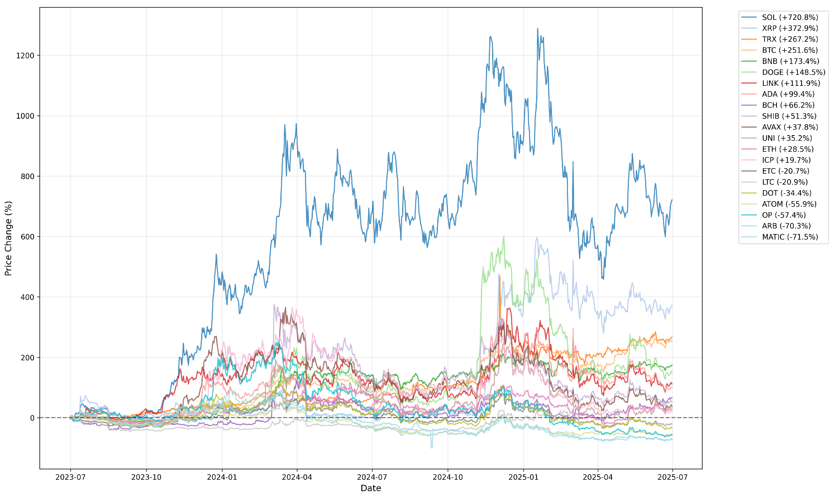
Figure 1 illustrates the trend in percentage growth rates from 30 June 2023 to 30 June 2025. Over this two-year period, SOL showed the highest growth at 720.8%, while MATIC experienced the lowest at −71.5%. Overall, ETC, LTC, DOT, ATOM, OP, ARB, and MATIC saw a decline, while the remaining assets showed growth.

Figure 1. Normalized Price Trends of Cryptocurrencies.

5. Experimental Results

This paper evaluates nine models on daily and hourly cryptocurrency closing price forecasts with a 7-step horizon. Our goal was to provide an accurate, multi-model benchmark.

We used a time-ordered evaluation protocol and a rolling window backtesting strategy to ensure our results were robust and free from data leakage. Models were trained and validated on historical data before being evaluated on a future-facing test set, guaranteeing that all reported metrics reflect out-of-sample performance.

For a fair comparison, each model was optimized for its unique architecture. We used AutoGluon’s automated tuning for the baselines and Chronos [22]. For TimeGPT, a proprietary closed-source LLM, we optimized its performance by controlling the number of iterations, allowing it to adapt to specific time series dynamics.

Figure 2 illustrates the optimal fine-tuning steps for TimeGPT across both Hourly and Daily datasets. We observed that BCH, BTC, ETC, SOL, TRX, and UNI required longer fine-tuning steps to achieve optimal results. In contrast, other cryptocurrencies yielded optimal results with shorter fine-tuning steps. This suggests that the data for these six cryptocurrencies may be more complex or exhibit stronger long-term dependencies.

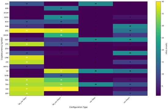
Figure 2. Optimal Fine-Tuning Steps for TimeGPT.

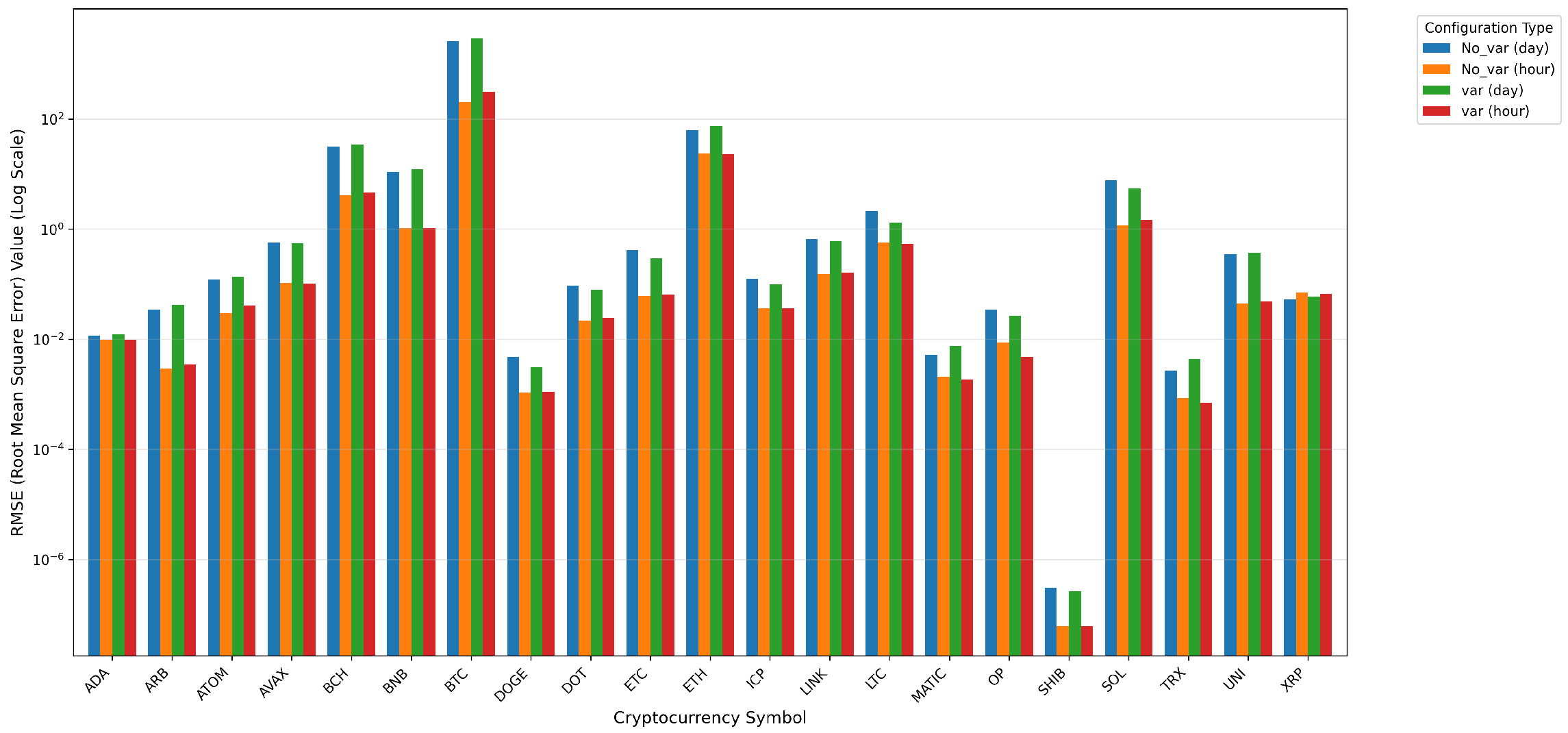
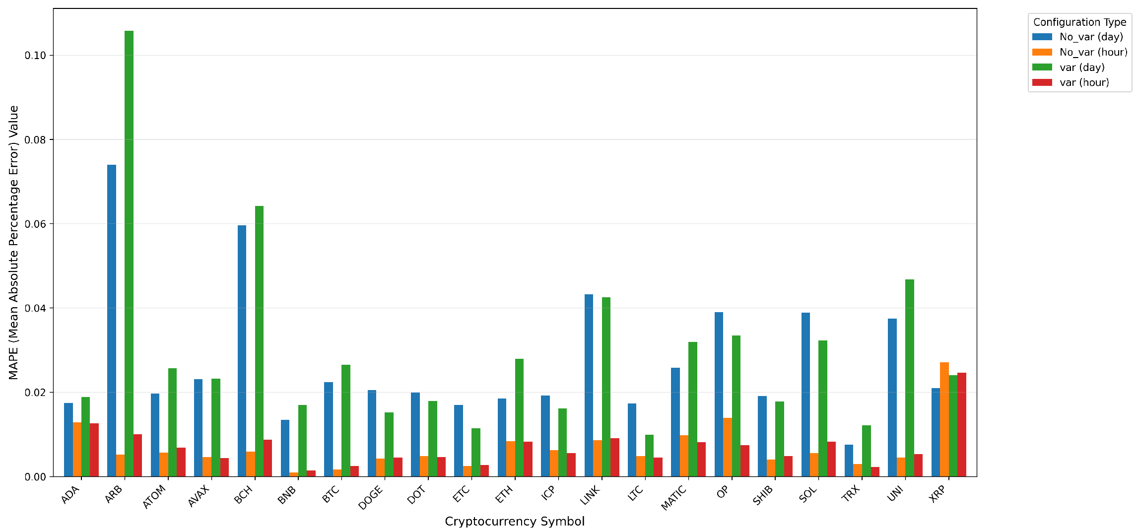
Figure 3, Figure 4 and Figure 5 show the MAE, RMSE, and MAPE of TimeGPT, divided under Daily and Hourly datasets according to whether variables are used or not. We find that in the Daily dataset, DOGE, DOT, ETC, ICP, LINK, LTC, OP, SHIB, and SOL become better after fine-tuning the results through the addition of variables, while the opposite is true for the other cryptocurrencies. In the hour dataset, ADA, AVAX, DOT, ETH, ICP, LTC, MATIC, OP, TRX and XRP have been fine-tuned by the addition of variables to give better results, while the opposite is true for the other cryptocurrencies. So, with the Daily and Hourly datasets, ICP, LTC, OP, and DOT all achieved better results after fine-tuning through the addition of variables, while the opposite was true for UNI, ATOM, BCH, ARB, and other cryptocurrencies, which had both good and bad results.

Figure 3. MAE Comparison for TimeGPT Fine-Tuning.

Figure 4. RMSE Comparison for TimeGPT Fine-Tuning.

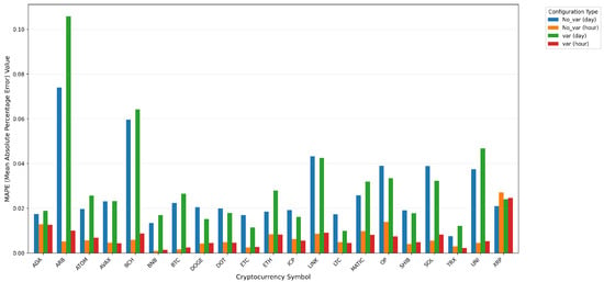
Figure 5. MAPE Comparison for TimeGPT Fine-Tuning.

Table 3 presents the average prediction metrics for all models across 21 cryptocurrencies, evaluated on both Hourly and Daily datasets. We primarily used Mean Absolute Percentage Error (MAPE) for a fair cross-asset comparison.

Table 3. Model Performance Metrics.

Model	MAE		RMSE		MAPE
	Day	Hour	Day	Hour	Day	Hour
ChronosFineTuned [bolt_small]	44.4355	27.6075	47.1465	31.1940	0.0412	0.0133
ChronosZeroShot [bolt_base]	50.0920	22.8800	61.9419	27.2580	0.0366	0.0081
DirectTabular	440.5986	33.6006	455.5468	34.9648	0.1319	0.0191
NPTS	1921.6443	93.0435	1807.7312	87.2644	0.4618	0.0303
PatchTST	201.4190	28.3949	216.2809	32.5368	0.0519	0.0107
RecursiveTabular	133.9992	26.5297	162.4802	32.9211	0.0475	0.0204
SeasonalNaive	173.8812	28.3835	200.4318	34.8499	0.0462	0.0210
TemporalFusionTransformer	280.1931	10.4450	289.1051	12.0893	0.0566	0.0139
TiDE	246.9273	80.0551	254.5326	82.4366	0.0496	0.0144
TimeGPT_No_var	139.0260	15.6999	150.4401	18.0468	0.0287	0.0078
TimeGPT_finetune_No_var	118.9567	9.8703	128.9118	11.0357	0.0273	0.0069
TimeGPT_finetune_var	141.2775	14.1517	144.8876	16.1225	0.0296	0.0070
TimeGPT_var	139.3994	14.5261	143.0434	16.7246	0.0293	0.0070

Note: The bold values in the table indicate the optimal result for that specific metric and model, signifying the best performance.

The optimally fine-tuned TimeGPT model without variables demonstrated the best overall performance, achieving the lowest average MAPE scores of 0.0273 on the Daily dataset and 0.0069 on the Hourly dataset. These results highlight the model’s superior accuracy and adaptability across a wide range of cryptocurrency data.

Interestingly, the effectiveness of fine-tuning and variables was highly context-dependent. While fine-tuning significantly improved the performance of the non-variable TimeGPT model, it had a nuanced, mixed impact when variables were included. Similarly, the Chronos model showed a contradictory result from fine-tuning: its MAE and RMSE improved significantly on the Daily dataset to 44.4355 and 47.1465, respectively, but its overall MAPE worsened. This finding underscores the importance of a multi-metric evaluation framework to fully assess a model’s true performance, as a single metric cannot capture the entire picture.

While average metrics (as shown in Table 3) provide an important macro-level view of model performance, they do not reveal the full picture of performance differences across various scenarios. To more accurately assess the models’ predictive capabilities, we employed the Diebold–Mariano (DM) test, with results presented in Table 4 (daily data) and Table 5 (hourly data). This test is a statistical method used to determine if the forecast accuracy of two models is significantly different. Its null hypothesis, that both models have the same predictive accuracy, can be rejected if the p-value is less than the significance level ($p<0.05$), allowing us to conclude that one model is statistically superior.

Table 4. Diebold–Mariano (DM) Test Results on MAPE (Day Data).

Base Model	TimeGPT Variant
	no_var	finetune_no_var	finetune_var	var
Chronos FT	AI: −4.49% SB: 66.7% SW: 33.3%	AI: 2.59% SB: 66.7% SW: 33.3%	AI: −6.59% SB: 61.9% SW: 33.3%	AI: −5.47% SB: 61.9% SW: 28.6%
Chronos ZS	AI: −4.90% SB: 42.9% SW: 33.3%	AI: 3.46% SB: 57.1% SW: 33.3%	AI: −3.90% SB: 47.6% SW: 33.3%	AI: −2.93% SB: 47.6% SW: 33.3%
DirectTabular	AI: 56.52% SB: 85.7% SW: 14.3%	AI: 59.46% SB: 85.7% SW: 14.3%	AI: 56.58% SB: 90.5% SW: 9.5%	AI: 57.02% SB: 90.5% SW: 9.5%
NPTS	AI: 75.12% SB: 90.5% SW: 9.5%	AI: 76.73% SB: 90.5% SW: 4.8%	AI: 76.64% SB: 90.5% SW: 4.8%	AI: 76.79% SB: 90.5% SW: 4.8%
PatchTST	AI: 36.99% SB: 85.7% SW: 14.3%	AI: 41.16% SB: 90.5% SW: 9.5%	AI: 35.70% SB: 81.0% SW: 14.3%	AI: 36.42% SB: 81.0% SW: 14.3%
RecursiveTabular	AI: 34.16% SB: 81.0% SW: 4.8%	AI: 39.09% SB: 95.2% SW: 4.8%	AI: 33.97% SB: 76.2% SW: 14.3%	AI: 34.43% SB: 76.2% SW: 9.5%
SeasonalNaive	AI: 37.77% SB: 95.2% SW: 4.8%	AI: 41.68% SB: 95.2% SW: 4.8%	AI: 37.41% SB: 90.5% SW: 9.5%	AI: 37.99% SB: 90.5% SW: 9.5%
TFT	AI: 24.13% SB: 71.4% SW: 19.0%	AI: 28.98% SB: 76.2% SW: 14.3%	AI: 26.10% SB: 66.7% SW: 19.0%	AI: 26.49% SB: 61.9% SW: 19.0%
TiDE	AI: 36.51% SB: 95.2% SW: 4.8%	AI: 40.60% SB: 95.2% SW: 4.8%	AI: 35.95% SB: 85.7% SW: 9.5%	AI: 36.54% SB: 85.7% SW: 9.5%

Notes: FT = Fine-tuned. ZS = Zero-shot. TFT = Temporal Fusion Transformer. The values are Average Improvement (AI), Significantly Better (SB), and Significantly Worse (SW). All comparisons are against the respective base Model, and the bolded AI value in each row represents the highest average improvement.

Table 5. Diebold–Mariano (DM) Test Results on MAPE (Hour Data).

Base Model	TimeGPT Variant
	no_var	finetune_no_var	finetune_var	var
Chronos FT	AI: 21.98% SB: 66.7% SW: 19.0%	AI: 36.27% SB: 85.7% SW: 9.5%	AI: 32.15% SB: 76.2% SW: 23.8%	AI: 31.41% SB: 76.2% SW: 23.8%
Chronos ZS	AI: -6.41% SB: 42.9% SW: 28.6%	AI: 13.42% SB: 71.4% SW: 19.0%	AI: 11.80% SB: 66.7% SW: 19.0%	AI: 10.65% SB: 61.9% SW: 23.8%
DirectTabular	AI: 37.09% SB: 81.0% SW: 19.0%	AI: 47.81% SB: 85.7% SW: 14.3%	AI: 48.90% SB: 90.5% SW: 9.5%	AI: 48.24% SB: 90.5% SW: 4.8%
NPTS	AI: 59.31% SB: 90.5% SW: 9.5%	AI: 63.67% SB: 95.2% SW: 4.8%	AI: 64.44% SB: 95.2% SW: 4.8%	AI: 64.32% SB: 95.2% SW: 4.8%
PatchTST	AI: 20.09% SB: 71.4% SW: 19.0%	AI: 33.10% SB: 81.0% SW: 14.3%	AI: 32.67% SB: 81.0% SW: 9.5%	AI: 31.97% SB: 85.7% SW: 9.5%
RecursiveTabular	AI: 48.34% SB: 85.7% SW: 9.5%	AI: 57.78% SB: 90.5% SW: 4.8%	AI: 57.90% SB: 95.2% SW: 4.8%	AI: 57.54% SB: 95.2% SW: 4.8%
SeasonalNaive	AI: 61.03% SB: 100.0% SW: 0.0%	AI: 67.08% SB: 100.0% SW: 0.0%	AI: 66.02% SB: 100.0% SW: 0.0%	AI: 65.72% SB: 100.0% SW: 0.0%
TFT	AI: 0.54% SB: 52.4% SW: 33.3%	AI: 15.66% SB: 66.7% SW: 23.8%	AI: 15.41% SB: 52.4% SW: 23.8%	AI: 14.48% SB: 57.1% SW: 28.6%
TiDE	AI: 29.38% SB: 85.7% SW: 9.5%	AI: 44.01% SB: 90.5% SW: 9.5%	AI: 44.27% SB: 90.5% SW: 9.5%	AI: 43.84% SB: 90.5% SW: 9.5%

Notes: FT = Fine-tuned. ZS = Zero-shot. TFT = Temporal Fusion Transformer. The values are Average Improvement (AI), Significantly Better (SB), and Significantly Worse (SW). All comparisons are against the respective base model, and the bolded AI value in each row represents the highest average improvement.

To further understand these differences, we also calculated the Average Improvement (AI) metric. This metric evaluates the degree to which one model is statistically and significantly superior to another. A positive percentage value indicates that TimeGPT’s error is lower than the other model’s, while a negative value indicates its error is higher.

We observed a significant phenomenon: in the DM test, the TimeGPT variant with the added variance feature demonstrated a stronger advantage against models like NPTS, RecursiveTabular, and DirectTabular, with a significantly higher Average Improvement (AI) value. This finding suggests that these baseline models may have inherent limitations in handling information such as volatility, extreme values, or trading volume. The endogenous variable features we added (e.g., analogous to open, high, low, and volume) effectively captured this information, allowing our model to compensate for these baselines’ weaknesses and achieve a significant leap in performance.

Interestingly, this advantage was less pronounced in comparison with the Chronos model. While the TimeGPT variant was still statistically superior to Chronos, its Average Improvement (AI) value was relatively lower. We hypothesize that this could be because Chronos, as a powerful pre-trained language model, already possesses the ability to implicitly learn and understand complex patterns like data volatility from raw time series. Consequently, the additional variance feature was redundant for Chronos, providing limited marginal gain and potentially introducing unnecessary noise, which slightly diminished its advantage in that comparison. In summary, our study not only demonstrated the uncontested leadership of the fine-tuned TimeGPT model without variables in terms of overall average error but, more importantly, it revealed that the effectiveness of features is context-dependent. No single "optimal" feature set can be applied to all models.

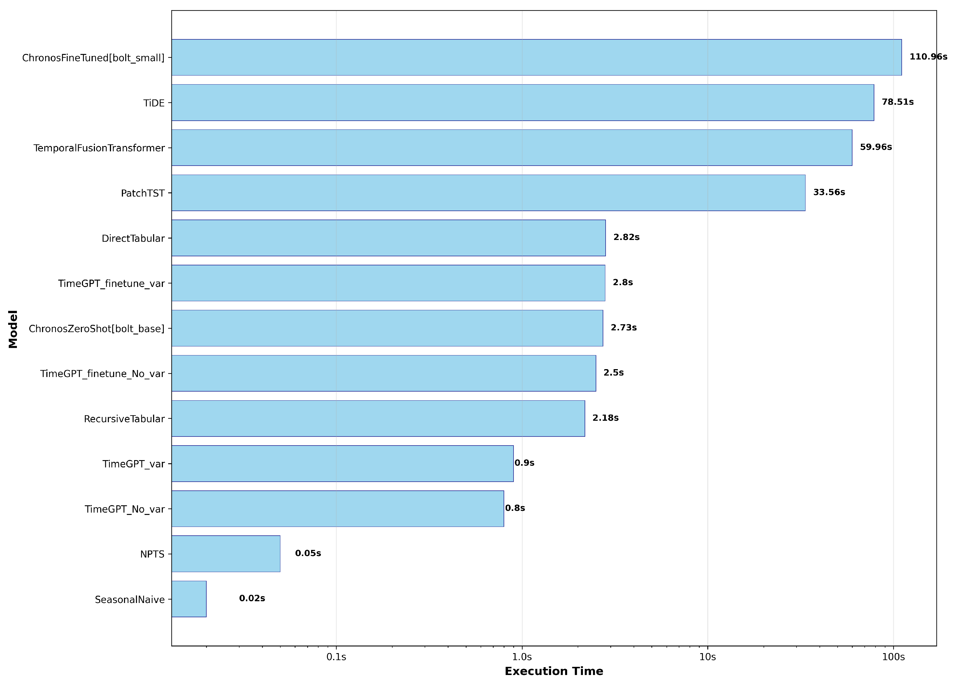
Figure 6 illustrates the total time required for models to generate predictions, encompassing both training and inference times. We observed that the total prediction times for the zero-shot models, TimeGPT and Chronos, are remarkably low, significantly outperforming deep learning models by an order of magnitude or more. When considering both Figure 6 and Table 3, it is evident that the optimally fine-tuned TimeGPT without additional variables achieved the best overall metrics in both Hourly and Daily datasets. Furthermore, this model produced predictions significantly faster than popular deep learning models such as TFT, TiDE, and PatchTST.

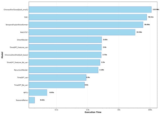
Figure 6. Model Timing Comparison Chart.

In our previous analysis, we established the technical leadership of models like TimeGPT without variables and Chronos based on their prediction accuracy and speed. However, a model’s true value is ultimately demonstrated by its ability to generate excess returns in a real market. To evaluate this, we used the Sharpe Ratio to measure economic value, analyzing performance under two trading strategies: long-only and long/short. It is important to note that the Sharpe Ratio calculation is based on 1-step-ahead price change prediction—essentially a classification or single-step forecasting task—which differs from our previous 7-step-ahead price trend forecasting.

The trading strategies were defined by simple, sign-based rules. For the long/short strategy, we adopted long positions when a price increase was predicted and short positions when a decrease was predicted. For the long-only strategy, we adopted long positions on a predicted price increase and held a cash position otherwise. Our positions were rebalanced at each time step based on the model’s latest prediction.

We selected BTC and ETH, the two cryptocurrencies with the highest market capitalization, as our subjects, which gives our analysis significant representativeness. During the analysis period (30 June 2024–30 June 2025), these two assets reflected two typical market states: BTC exhibited a strong cyclicality and upward trend, representing a relatively mature and stable market, while ETH underwent a large-scale drawdown and sharp volatility, representing a more challenging and complex market environment. By comparing the models’ performance across these two distinct market characteristics, we can more comprehensively evaluate their robustness and applicability.

Based on our analysis of the data in Table 6, we uncovered a key finding: a model’s effectiveness is not universal but is highly dependent on its ability to match specific market characteristics, and there is not a simple linear relationship between prediction accuracy and actual economic value.

Table 6. Comparison of ETH and BTC Sharpe Ratio Results for Different Strategies.

Model	Long-Only Strategy		Long/Short Strategy
	ETH SR	BTC SR	ETH SR	BTC SR
Chronos	−0.5789	1.2853	−0.7639	1.0296
DirectTabular	0.7188	0.3565	1.1915	−0.9114
NPTS	0.2070	0.3846	0.4491	−1.0395
PatchTST	−0.8138	−0.0386	−1.0519	−1.3850
RecursiveTabular	−0.4732	0.5507	−0.5973	−0.5343
SeasonalNaive	−0.0070	1.5388	0.0860	0.8594
timegpt_finetune_no_var	0.3180	0.9732	0.6317	0.1740
timegpt_finetune_var	2.5438	1.2337	4.2947	0.3506

Note: The bold values in the table indicate the optimal result.

Taking the TimeGPT model as an example, the version using variables showed astonishing profitability on ETH, with a Sharpe Ratio as high as 4.2947 under the long/short strategy. This proves that in ETH’s highly volatile market, variables provide crucial signals that can significantly enhance the model’s economic value. Conversely, in the relatively stable BTC market, the same model performed averagely, indicating that additional variable information may be of limited value.

In contrast, the zero-shot Chronos model performed best on BTC, with its pre-trained architecture appearing to be more adept at capturing the long-term trends and cyclicality of the BTC market. This further emphasizes the critical importance of a model’s fit with market characteristics.

This phenomenon also highlights the difference between the prediction task and economic value. Although the version not using variables had the lowest average error in 7-step-ahead forecasting, its Sharpe Ratio in 1-step-ahead predictions was inferior to those models that could more effectively utilize market dynamics (through variables or cyclicality). This suggests that the role of variables becomes more critical when the prediction task changes from multi-step trend forecasting to single-step price change prediction.

Given the highly volatile nature of the cryptocurrency market and its demand for rapid response times, relying solely on prediction accuracy scores, as is common in prior research, presents limitations in evaluating forecasting model efficacy. We propose that model evaluation should integrate both prediction speed and accuracy scores.

Our analysis, backed by the Diebold–Mariano (DM) test, confirmed the statistical superiority of the optimally fine-tuned TimeGPT without variables. This model achieved the lowest average error metrics and demonstrated a significant statistical advantage over other models across both the Hourly and Daily datasets. Following closely, the zero-shot Chronos model also showed strong performance, providing a robust, out-of-the-box solution.

However, the analysis of Sharpe Ratios revealed a deeper layer of model performance. While the TimeGPT model without variables excelled in terms of average prediction accuracy, its economic value did not always surpass models that effectively utilized specific market characteristics. The zero-shot Chronos model, for example, proved to be the superior choice for the BTC market, where it leveraged its pre-trained architecture to capture long-term trends and cyclicality, leading to high-performing trading strategies. In contrast, the TimeGPT model with variables showed a significant advantage in the highly volatile ETH market, where its ability to incorporate dynamic market data resulted in an outstanding Sharpe Ratio.

Overall, the optimally fine-tuned TimeGPT without variables demonstrates superior results and exceptionally fast prediction speeds across both Daily and Hourly interval datasets for all 21 cryptocurrencies, making it a compelling choice for a balanced approach to accuracy and efficiency. Our research highlights that a comprehensive evaluation framework, which includes statistical tests and economic value metrics alongside traditional accuracy scores, is essential for a more complete understanding of a model’s true effectiveness.

6. Conclusions

This study comprehensively evaluates nine baseline, zero-shot, and deep learning models on 21 cryptocurrency prediction tasks, aiming to provide investors and market participants with efficient and accurate forecasting strategies. Our key findings are as follows.

The TimeGPT model (without variables, optimally fine-tuned) demonstrated exceptional performance across both Daily and Hourly datasets, achieving the best prediction results. Our research confirmed this conclusion from a statistical standpoint through the Diebold–Mariano (DM) test, which showed this model to be significantly superior in error metrics to most other models, indicating its strong adaptability and generalization capabilities. The fine-tuned Chronos model performed well on the Daily dataset but saw its performance decline on the Hourly dataset, suggesting it may be more suitable for longer-term predictions.

Our research also revealed that variables have a significantly differentiated impact on the prediction performance of various cryptocurrencies. For assets such as ICP, LTC, OP, and DOT, introducing variables improved prediction performance on both Daily and Hourly datasets. However, for others like UNI, ATOM, BCH, and ARB, performance deteriorated. This finding emphasizes that the effectiveness of features like OHLCV (Open, High, Low, Close, Volume) and Moving Averages is not universal; their selection and combination require a targeted approach based on the specific prediction time interval and the characteristics of the crypto asset.

In terms of prediction speed, zero-shot models like TimeGPT and Chronos were tens of times faster than traditional deep learning models, significantly enhancing computational efficiency while maintaining high accuracy. Notably, on the Hourly dataset, the optimally fine-tuned TimeGPT not only achieved the best prediction metrics but also delivered results at a speed that is crucial in the fast-paced cryptocurrency market.

Beyond prediction accuracy and speed, our Sharpe Ratio analysis further revealed the models’ actual economic value, leading to the important conclusion that a model’s effectiveness is highly dependent on its fit with specific market characteristics. For example, the TimeGPT model (using variables) showed astonishing profitability in the highly volatile ETH market, with a Sharpe Ratio as high as 4.2947. In contrast, the zero-shot Chronos model performed best in the highly cyclical BTC market, with a Sharpe Ratio of 1.0296. This indicates that although the TimeGPT without variables was the best in terms of average error, its economic value was not always the highest, as different models can capture unique profit opportunities in different market environments.

Overall, the optimally fine-tuned TimeGPT (without variables) achieved the best comprehensive performance (balancing accuracy and speed) across both Daily and Hourly datasets for all 21 cryptocurrencies, making it a compelling choice for a balanced approach to accuracy and efficiency. Given the high volatility and strict real-time requirements of the cryptocurrency market, this study, by applying a multi-dimensional evaluation methodology that combines prediction speed with accuracy, provides a more comprehensive and practically guiding standard for evaluating financial time series forecasting models. TimeGPT, by delivering top-tier prediction results at speeds far exceeding its counterparts, will undoubtedly greatly assist cryptocurrency investors and participants in quickly obtaining high-quality forecasts, thereby more effectively mitigating potential risks and seizing market opportunities.

References

- CoinMarketCap. Cryptocurrency Prices, Charts and Market Caps. Available online: https://coinmarketcap.com (accessed on 9 July 2025).
- Stosic, D.; Stosic, D.; Ludermir, T.B.; Stosic, T. Exploring disorder and complexity in the cryptocurrency space. Phys. A Stat. Mech. Its Appl. 2019, 525, 548–556. [Google Scholar] [CrossRef]
- Dimpfl, T.; Peter, F.J. Nothing but noise? Price discovery across cryptocurrency exchanges. J. Financ. Mark. 2021, 54, 100584. [Google Scholar] [CrossRef]
- Lim, B.; Arık, S.Ö.; Loeff, N.; Pfister, T. Temporal fusion transformers for interpretable multi-horizon time series forecasting. Int. J. Forecast. 2021, 37, 1748–1764. [Google Scholar] [CrossRef]
- Das, A.; Kong, W.; Leach, A.; Mathur, S.; Sen, R.; Yu, R. Long-term forecasting with tide: Time-series dense encoder. arXiv 2023, arXiv:2304.08424. [Google Scholar] [CrossRef]
- Nie, Y.; Nguyen, N.H.; Sinthong, P.; Kalagnanam, J. A time series is worth 64 words: Long-term forecasting with transformers. arXiv 2022, arXiv:2211.14730. [Google Scholar] [CrossRef]
- Garza, A.; Mergenthaler-Canseco, M. TimeGPT-1. arXiv 2023, arXiv:2310.03589. [Google Scholar] [CrossRef]
- Ansari, A.F.; Stella, L.; Turkmen, C.; Zhang, X.; Mercado, P.; Shen, H.; Shchur, O.; Rangapuram, S.S.; Arango, S.P.; Kapoor, S.; et al. Chronos: Learning the Language of Time Series. arXiv 2024, arXiv:2403.07815. [Google Scholar] [CrossRef]
- García-Medina, A.; Aguayo-Moreno, E. Lstm–garch hybrid model for the prediction of volatility in cryptocurrency portfolios. Comput. Econ. 2024, 63, 1511–1542. [Google Scholar] [CrossRef] [PubMed]
- Li, D.; Sun, G.; Miao, S.; Gu, Y.; Zhang, Y.; He, S. A short-term electric load forecast method based on improved sequence-to-sequence gru with adaptive temporal dependence. Int. J. Electr. Power Energy Syst. 2022, 137, 107627. [Google Scholar] [CrossRef]
- Liu, T.; Wang, Y.; Sun, J.; Tian, Y.; Huang, Y.; Xue, T.; Li, P.; Liu, Y. The role of transformer models in advancing blockchain technology: A systematic survey. arXiv 2024, arXiv:2409.02139. [Google Scholar] [CrossRef]
- Sun, X.; Liu, M.; Sima, Z. A novel cryptocurrency price trend forecasting model based on LightGBM. Financ. Res. Lett. 2020, 32, 101084. [Google Scholar] [CrossRef]
- Rao, K.R.; Prasad, M.L.; Kumar, G.R.; Natchadalingam, R.; Hussain, M.M.; Reddy, P.C.S. Time-series cryptocurrency forecasting using ensemble deep learning. In Proceedings of the 2023 International Conference on Circuit Power and Computing Technologies (ICCPCT), Kollam, India, 10–11 August 2023; IEEE: New York, NY, USA, 2023; pp. 1446–1451. [Google Scholar] [CrossRef]
- Murray, K.; Rossi, A.; Carraro, D.; Visentin, A. On forecasting cryptocurrency prices: A comparison of machine learning, deep learning, and ensembles. Forecasting 2023, 5, 196–209. [Google Scholar] [CrossRef]
- Belcastro, L.; Carbone, D.; Cosentino, C.; Marozzo, F.; Trunfio, P. Enhancing cryptocurrency price forecasting by integrating machine learning with social media and market data. Algorithms 2023, 16, 542. [Google Scholar] [CrossRef]
- Lee, M.C. Temporal Fusion Transformer-Based Trading Strategy for Multi-Crypto Assets Using On-Chain and Technical Indicators. Systems 2025, 13, 474. [Google Scholar] [CrossRef]
- Wang, M.; Braslavski, P.; Manevich, V.; Ignatov, D.I. Bitcoin Ordinals: Bitcoin Price and Transaction Fee Rate Predictions. IEEE Access 2025, 13, 35478–35489. [Google Scholar] [CrossRef]
- Zhou, W.-X.; Mu, G.-H.; Chen, W.; Sornette, D. Investment strategies used as spectroscopy of financial markets reveal new stylized facts. PLoS ONE 2011, 6, e24391. [Google Scholar] [CrossRef]
- Das, A.; Kong, W.; Sen, R.; Zhou, Y. A decoder-only foundation model for time-series forecasting. In Proceedings of the 41st International Conference on Machine Learning, Vienna, Austria, 21–27 July 2024; PMLR, 2024; pp. 10148–10167. [Google Scholar] [CrossRef]
- Diebold, F.X.; Mariano, R.S. Comparing predictive accuracy. J. Bus. Econ. Stat. 2002, 20, 134–144. [Google Scholar] [CrossRef]
- Sharpe, W.F. Mutual fund performance. J. Bus. 1966, 39, 119–138. [Google Scholar] [CrossRef]
- Erickson, N.; Mueller, J.; Shirkov, A.; Zhang, H.; Larroy, P.; Li, M.; Smola, A. AutoGluon-Tabular: Robust and Accurate AutoML for Structured Data. arXiv 2020, arXiv:2003.06505. [Google Scholar] [CrossRef]
Disclaimer/Publisher’s Note: The statements, opinions and data contained in all publications are solely those of the individual author(s) and contributor(s) and not of MDPI and/or the editor(s). MDPI and/or the editor(s) disclaim responsibility for any injury to people or property resulting from any ideas, methods, instructions or products referred to in the content. |
© 2025 by the authors. Licensee MDPI, Basel, Switzerland. This article is an open access article distributed under the terms and conditions of the Creative Commons Attribution (CC BY) license (https://creativecommons.org/licenses/by/4.0/).