Article

Improving Dry-Bulb Air Temperature Prediction Using a Hybrid Model Integrating Genetic Algorithms with a Fourier–Bessel Series Expansion-Based LSTM Model

1
UniSQ College, University of Southern Queensland, Springfield, QLD 4350, Australia
2
Department of Cybersecurity, Technical College of Engineering, Al-Ayen Iraqi University, Nasiriyah 64001, Thi-Qar, Iraq
3
Faculty of Sustainable Design Engineering, University of Prince Edward Island, Charlottetown, PE C1A 4P3, Canada
4
Artificial Intelligence Applications Laboratory, School of Mathematics, Physics, and Computing, University of Southern Queensland, Springfield, QLD 4300, Australia
5
Department of Mathematics and Statistics, Faculty of Science, King Faisal University, P.O. Box 400, Al-Ahsa 31982, Saudi Arabia
6
Canadian Centre for Climate Change and Adaptation, University of Prince Edward Island, St Peters, PE C1A 4P3, Canada
*
Authors to whom correspondence should be addressed.
Forecasting 2025, 7(3), 46; https://doi.org/10.3390/forecast7030046
Submission received: 25 July 2025 / Revised: 13 August 2025 / Accepted: 26 August 2025 / Published: 29 August 2025
(This article belongs to the Section Environmental Forecasting)

Abstract

The dry-bulb temperature is a critical parameter in weather forecasting, agriculture, energy management, and climate research. This work proposes a new hybrid prediction model (FBSE-GA-LSTM) that integrates the Fourier–Bessel series expansion (FBSE), genetic algorithm (GA), and long short-term memory (LSTM) networks together to predict the dry-bulb air temperature. The hybrid model FBSE-GA-LSTM utilises the FBSE to decompose time series data of interest into an attempt to remove the noise level for capturing the dominant predictive patterns. Then, the FBSE is embedded into the GA method for the best feature selection and dimension reduction. To predict the dry-bulb temperature, a new model (FBSE-GA-LSTM) was used by hybridising a proposed model FBSE-GA with the LSTM model on the time series dataset of two different regions in Saudi Arabia. For comparison, the FBSE and GA models were hybridised with a bidirectional LSTM (BiLSTM), gated recurrent unit (GRU), and bidirectional gated recurrent unit (BiGRU) models to obtain the hybrid FBSE-GA-BiLSTM, FBSE-GA-GRU, and FBSE-GA-BiGRU models along with their standalone versions. In addition, benchmark models, including the climatic average and persistence approaches, were employed to demonstrate that the proposed model outperforms simple baseline predictors. The experimental results indicated that the proposed hybrid FBSE-GA-LSTM model achieved improved prediction performance compared with the contrastive models for the Jazan region, with a mean absolute error (MAE) of 1.458 °C, a correlation coefficient (R) of 0.954, and a root mean squared error (RMSE) of 1.780 °C, and for the Jeddah region, with an MAE of 1.459 °C, an R of 0.952, and an RMSE of 1.782 °C, between the predicted and observed values of dry-bulb air temperature.

1. Introduction

The dry-bulb temperature (DBT) is a critical weather parameter which is used as a representative of temperature for many applications such as environmental monitoring of industrial and agricultural processes. It is the temperature of the air as measured by a thermometer freely exposed to the air but shielded from radiation and moisture. The accurate prediction of DBT is important in several domains such as weather forecasting, the analysis of climate change, and the management of renewable energy, and precision agriculture DBT predictions contribute to energy optimisation, building climate control as well as natural disaster preparations [1,2].
In the literature, DBT estimations have been traditionally based on the numerical weather prediction (NWP) model and statistical methodologies, for example on autoregressive integrated moving averages (ARIMA) or regression methods [3]. Although these are widely applied techniques, it is frequently difficult for these techniques to effectively represent non-linear, highly complex, and dynamically interacting influences on meteorological variables [4]. This limitation has led to the investigation and application of advanced artificial intelligence (AI) and machine learning (ML) tools to improve the accuracy of predictions [5,6].
Significant recent advances in deep learning (DL) have made DBT prediction more accurate through big data solutions to recognise the highly complex patterns of atmosphere behaviour. In the last few years, there has been an increasing use of machine learning (ML) for DBT prediction, especially since the conventional statistical methods have shortcomings in dealing with nonlinear relationships between input–output variables, and the temporal relationships between the variables in climatic time series.
Among these models, artificial neural networks (ANNs), the convolutional neural network (CNN), recurrent neural networks (RNNs), and long short-term memory (LSTM) have demonstrated a lot of potential. ANNs have been heavily utilised in DBT prediction because of their capacity to model complex, nonlinear relationships. For example, Gündoğdu and Elbir [7] used a feedforward ANN to forecast maximum daily temperatures and better results were obtained compared to regression-based approaches. Similarly, Tehrani et al., [8] used ANN models to predict hourly temperatures in urban areas, obtaining high accuracy in the representation of short-term DBT variability. Currently LSTM networks (an RNN variant that captures long-term dependencies) have been established as being some of the best methods for DBT prediction. Hasan et al., [9] used LSTM models with features including humidity, solar radiation, and wind speed to forecast the daily DBT with substantial enhancements in the accuracy of prediction. Huang et al., [10] found that LSTM models could successfully manage nonstationary temperature patterns to be applicable in long-term climate interpretation. Yet independent ML and DL models can be ineffective toward noisy imaging data because they are restricted by their own model capacity, and they may not entirely represent subtle nuances in DBT [11].
In order to overcome these issues, hybrid modelling paradigms have been considered as the more promising alternative. In recent works, excellent results have been achieved by coupling signal processing methods such as multivariate variational mode decomposition (MVMD), with state-of-the-art neural network designs such as the bidirectional long short-term memory (BiLSTM) networks. To improve the accuracy of temperature prediction, in recent years, some signal decomposition methods have been widely used for preprocessing the nonstationary and nonlinear time series data inputs for the machine learning or deep learning models in the era of signal processing and data science technology. Decomposition methods aim at decomposing complex climate signals into simpler sub-structures which have more stable statistical properties to facilitate the physical interpretation of a model prediction. Empirical mode decomposition (EMD) is one of the early adaptive decomposition techniques used in this regard. It is a versatile instrument to perform signal decomposition into the IMFs without a predetermined set of basis functions [12]. However, mode mixing and noise degradation are two drawbacks of EMD. Ensemble empirical mode decomposition (EEMD) was proposed to solve these problems, which adds white noises to cut down the mode mixing and improve stability [13]. Further developments, such as the improvement based on the complete ensemble empirical mode decomposition with adaptive noise [14], have enhanced the robustness and the accuracy of the decomposition of signals. Wavelet transform (WT) and discrete wavelet transform (DWT) are other methods that have been extensively used for predicting DBT. These models decompose a time series into multiple time resolutions based on fixed basis functions and are well suited to capturing localised features in non-stationary data [15]. However, unlike EMD-based approaches, wavelet techniques necessitate a priori choice of the wavelet basis and this can be too restrictive for real-time implementations, as new wavelet representations are to be selected each time new segments of the learning data are processed.
More recently, variational mode decomposition (VMD) and its multivariate extension MVMD has been presented to accomplish this task. VMD formulates the decomposition as an optimisation problem, thereby improving the mode mixing and ensuring a compacted and band-limited modes [16]. An extension of MVMD allows joint decomposition of the multivariate signals, retaining the inter-channel dependencies and gaining improved performance in multi-sensor and multivariate problem predictions [17]. Multivariate empirical mode decomposition (MEMD) is another approach to process multichannel data with shared modes among the signals, to increase interpretability in multivariate systems [18]. These approaches of decomposition together with the advanced deep learning models like BiLSTM, have shown to be successful in improving prediction performance. For instance, Tang et al., [19] utilised VMD with BiLSTM for the hourly temperature forecast and demonstrated great improvement on the forecasting accuracy compared with raw-data-based models. Similarly, Ahmed et al., [20] also suggested EEMD-BiLSTM for air temperature forecasting and demonstrated that hybrid decomposition and deep learning models were able to handle both seasonal patterns and non-linear relations. These findings highlight the importance of decomposition methods as a pre-processing stage for modern temperature predictors in which the deep learning models can work over thousands of more regularised and interpretable signals. These hybrid methods provide further improvement in the forecasting accuracy since complex signals can be effectively decomposed by those methods, noise is reduced, and critical temperature patterns are preserved [21,22]. Through this comparison, it was shown that the hybrid models that combine the ML and DL models performed the best for DBT prediction. For example, Zhou et al., [23] developed an HBA-optimised hybrid ANN model which is denoted as HBA-ANN. They compared HBA-ANN model with the classical ANN and gene expression programming (GEP) models to predict DBT in extreme regions, the Furnace Creek Death Valley, USA, and Vostok Station, Antarctica. Within the prediction horizons of 1–3 months, the HBA-ANN model performed better than the benchmark models. Comparison on the performance of this approach versus their counterparts’ classical artificial neural networks (ANN) and RNN were performed. They employed a genetic algorithm (GA) for meta-learning to optimise abstract network architecture selection as well. They confirmed that the GA–LSTM hybrid model was better than the ML and DL models. One such contemporary hybrid model is the combination of CNN and LSTM, termed as CNN-LSTM. This is to take advantage of the CNN’s property to process low dimensional time series data and the LSTM’s ability to learn long distance relationships to capture temporal patterns present in wide datasets (i.e., large temperature datasets). In [24], authors showed that CNN-LSTM outperformed CNN and LSTM for daily DBT forecast at the John F. Kennedy International Airport (New York). Similarly, Hou et al., [25], using CNN-LSTM tightening methods, presented a better hourly DBT forecasting accuracy in Yinchuan, China. The superiority of hybrid deep learning models is justified also by the integration of pre-processing methods to enhance the model performance [26]. In this paper, we attempt to construct an accurate prediction model for the DBT prediction problem and exploit the combination of the hybrid models derived from the FBSE, genetic algorithm (GA), and long short-term memory (LSTM) networks. We investigate the performance of the hybrid model FBSE-GA-LSTM and other deep learning model structures in the context of DBT prediction at various horizon lengths (i.e., one hourly/monthly/weekly ahead horizon) [27]. The performances of the proposed FBSE-GA-BLSTM models were tested across various evaluation metrics such as root mean square error (RMSE), mean absolute error (MAE), correlation coefficient (R), linear model efficiency (LME), and relative percentage error (RPE) to critically measure the correctness of predictions from different perspectives.
Previous studies have demonstrated the potential of hybrid models for improving weather prediction accuracy; however, many have been limited by suboptimal noise handling, inadequate feature selection, or insufficient evaluation against naïve benchmarks. The proposed FBSE-GA-LSTM framework addresses these gaps by integrating Fourier–Bessel series expansion (FBSE) for effective noise reduction and extraction of dominant predictive patterns, genetic algorithm (GA) for optimal feature selection and dimensionality reduction, and long short-term memory (LSTM) networks for capturing temporal dependencies in the data. Unlike earlier approaches, the present model has been systematically compared with both advanced deep learning hybrids (FBSE-GA-BiLSTM, FBSE-GA-GRU) and simple baseline predictors (persistence and climatic average), demonstrating superior predictive performance across two distinct climatic regions. This design not only enhances accuracy but also provides robustness in forecasting highly repetitive variables such as the dry-bulb temperature.

2. Materials and Methods

2.1. Dataset and Study Location

The data used in this study were collected from selected areas in the Kingdom of Saudi Arabia as shown in Figure 1. These data were retrieved from the Department of Meteorology, ranging from the period of 1978 to 2013 on daily basis. Jazan is located in the southwest of Saudi Arabia at about 16.8892° N latitude and 42.5511° E longitude with a tropical type of climate. In Jazan, temperatures always remain slightly high during all year, complimented by moderate humidity. Jazan City experiences a hot, humid summer with temperatures exceeding 40 °C, but relatively mild winters with temperatures not dropping below 20 °C and monsoon-like rains which occur during June to September when Jazan receives heavy rainfall, contributing to vegetative growth and crop productivity. The topographical nature of Jazan includes coastal, plain, and mountainous areas, forming valleys. All along the coast of the Red Sea, one can see sandy beaches and low-lying areas. The mountains of the SAWARAT range the picturesque hills parallel to the sea lines and change weather of the area by varying the temperature and precipitation. Transport Jazan is situated in a region of Saudi Arabia which is of great strategic importance regarding trade as well as an access point to the rest of the Arabian Peninsula. Jeddah lies along the western coast of Saudi Arabia at the coordinates 21.2854° N 39.2376° E. The city has a desert climate with blistering summer heat (with temperatures often exceeding 40 °C) and mild winters (with temperatures dropping to 15 °C). Jeddah encounters limited precipitation, predominantly during the winter season. Nonetheless, the summer months are marked by elevated humidity levels attributable to its coastal geography. The city is susceptible to flash flooding during infrequent heavy precipitation events, primarily due to the presence of adjacent wadis (dry riverbeds) and minor valleys. Jeddah functions as a significant port and commercial centre, establishing a connection between the Kingdom and international markets, thereby facilitating trade and economic activities.
A geographical overview of the research region is illustrated in Figure 1, highlighting the positions of the meteorological stations located in Jazan and Jeddah.
The dataset consisted of various input variables recorded at daily intervals. These variables included the mean wind speed, maximum wind direction, maximum wind speed, timing of the maximum wind speed, mean station-level pressure, mean sea level pressure, mean relative humidity, mean vapour pressure, mean sky cover (measured in oktas), maximum station-level pressure, maximum sea level pressure, maximum air temperature (dry bulb), maximum air temperature (wet bulb), maximum relative humidity, minimum station-level pressure, minimum sea level pressure, minimum air temperature (dry bulb), minimum air temperature (wet bulb), minimum relative humidity, total rainfall, SynOps hours, four primary synoptic observations, individual synoptic observations, and mean air temperature (wet bulb). Figure 2 presents a summary and descriptive analysis of the data utilised in this study.

2.2. The Proposed Model

In this study, we adopted three distinct modelling methods based on the Fourier–Bessel series expansion, genetic algorithm and the long short-term memory network models to improve the prediction of dry-bulb air temperature. The details of the model development methodology are given below.

2.2.1. Fourier–Bessel Series Expansion (FBSE)

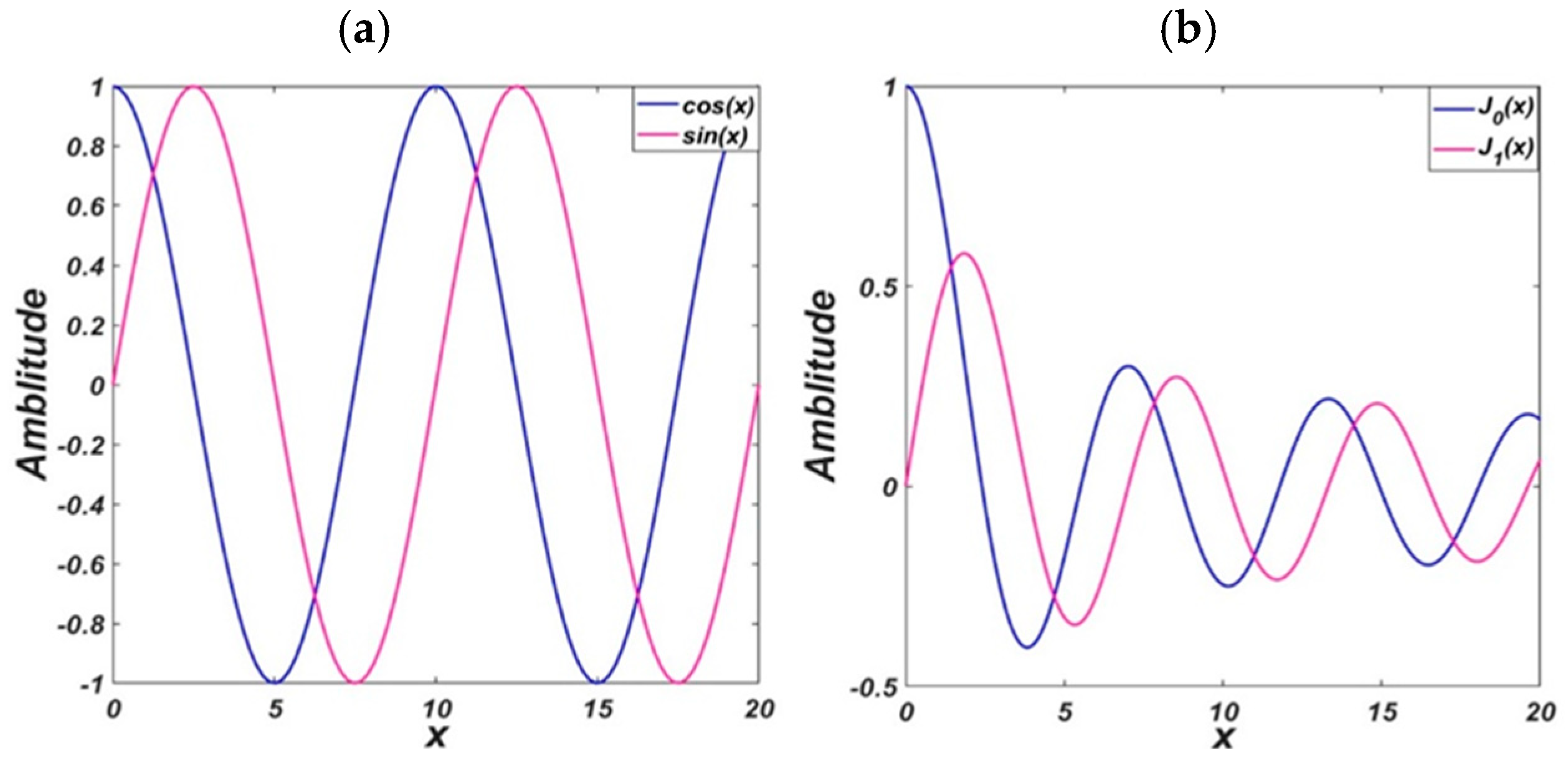
FBSE has been well-applied to non-stationary signal analysis [27], and many works show the great advantages of FBSE compared to FFT. Firstly, compared with Fourier transform (FT), the FBSE method does not require a window function for spectrum analysis. Second, the FBSE has two-time interval processing and the DFT length is the same as the signal length of the filter that produces coefficients. When we compared the Bessel function (BF) with the FT, it is shown in Figure 3 that the BF was non-stationary and had amplitude modulation. Most importantly, in contrast to FBSE, which uses the non-stationary BF, the FT uses the stationary BF, according to [27], the FBSE in fact can offer and achieve a more compact representation than the FT, and the FBSE method has obtained a good frequency resolution compared with the FT. Dash et al. [28] when analysing non-stationary signals, showed that the FBSE coefficients were unique and had a better spectral resolution than FT, with the number of unique FBSE coefficients needed for representation of the spectrum being equal to the length of the discrete time signal, in contrast to FFT which was two times the length of the discrete time signal.
The Fourier–Bessel series expansion’s fundamental idea is that any function can be expressed as the sum of Bessel functions. Friedrich Bessel was a German mathematician who first studied them in the early 19th century, and thus it was named after him. The second-order differential Bessel equation has a regular singular point at the origin. Bessel functions are solutions to this differential equation. The second-order ordinary differential equation of the following form is Bessel’s equation of order α (with α ≥ 0):
x 2 z + x z + x 2 α 2 z = 0
The general solution of Equation (1) is
z x = A J α x + B Z α x
where α = 0, 1, 2,…, is the Bessel function’s order, A and B are constants, and the J α x   and Z α x   are the solutions to this equation and are referred to as Bessel functions of the first and second kinds, respectively. The solutions to the Bessel differential Equation (2) are Bessel functions J α x of the first type of order α, which are also referred to as cylindrical functions. For the negative non-integer α, these solutions diverge as x approaches zero, but for integer or positive α, they are finite at x = 0. The Bessel differential equation of order zero is a second-order ordinary differential Equation with the following formula:
  x 2 z + x z + x 2 z = 0
By extending Bessel functions, a function can be expressed in terms of Bessel functions of a specific type and order. The Fourier–Bessel series expansion, which represents a function in terms of Bessel functions of the first class, is a frequently used example. The formula for this type of expansion is as follows:
f x =   i = 1   C i J α x   z i
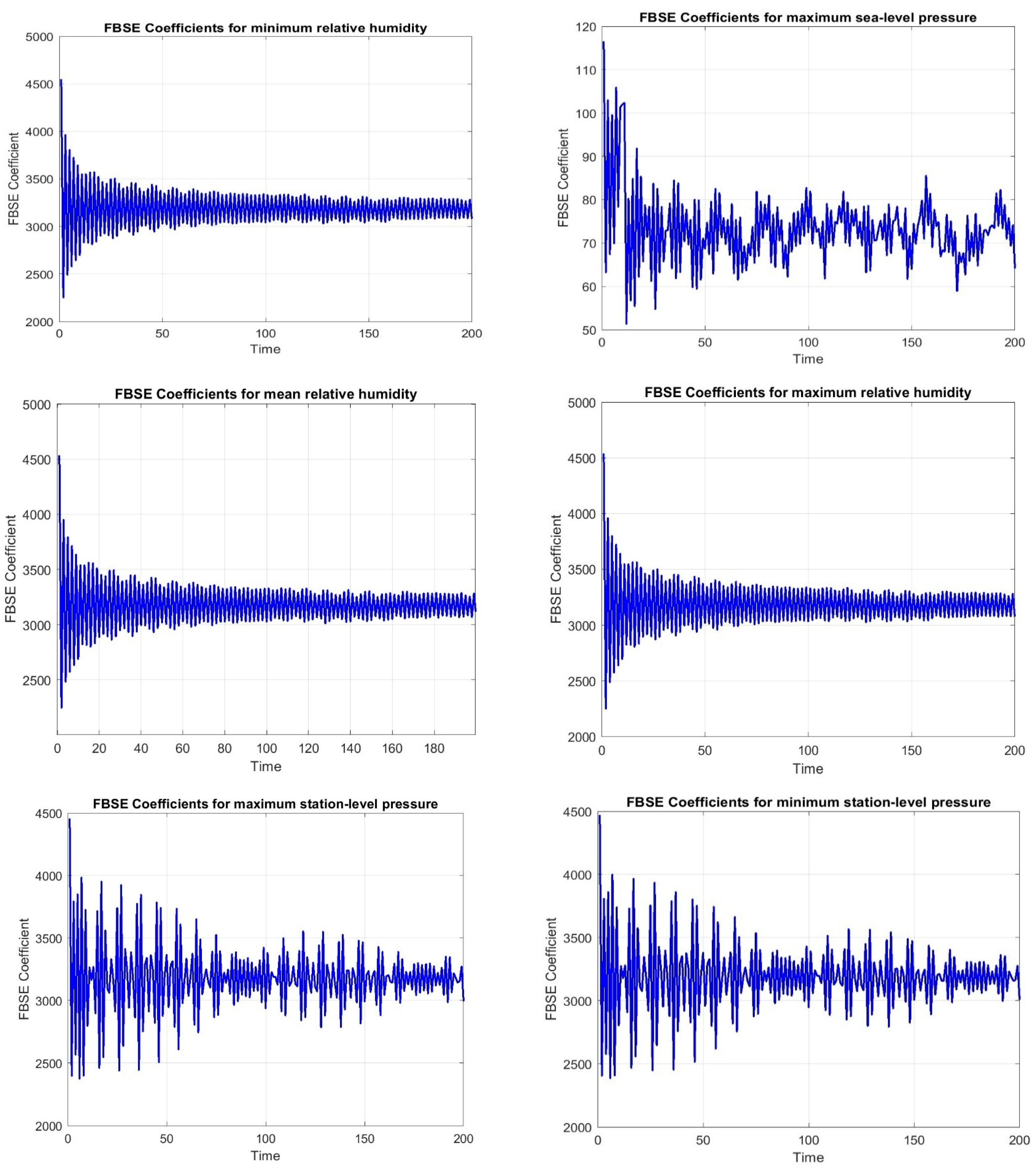
where   z i denotes the positive roots and C i   denotes the expansion’s coefficients. Usually, the orthogonality characteristics of the Bessel functions—such as the orthogonality integral are used to derive the coefficient C i   . There are also other types of Bessel function expansions. For instance, the Fourier–Bessel series makes use of the Bessel function of the second kind Zα(x). The Fourier–Bessel transform which is an effective method for the investigation of functions in the frequency domain can be carried out by the Fourier–Bessel series. To analyse the spectral content of a function, the Fourier–Bessel transform can be used to decompose a process into a sum of Bessel functions and their coefficients [28]. In signal processing, the Fourier–Bessel series is an expansion of functions in terms of Bessel functions. Bessel functions are chosen as the basic functions in the Fourier–Bessel series expansion, based on their orthogonality property (which will be explained later), to allow the series to converge to the original function in a suitable domain. The Bessel functions are used by the FBSE mainly due to their orthogonality. The recurrence relation of the Bessel function is also used to compute the Fourier–Bessel transform and its inverse, which improves computation efficiency [28]. Figure 4 shows FBSE coefficients for the different variables.

2.2.2. Genetic Algorithm (GA)

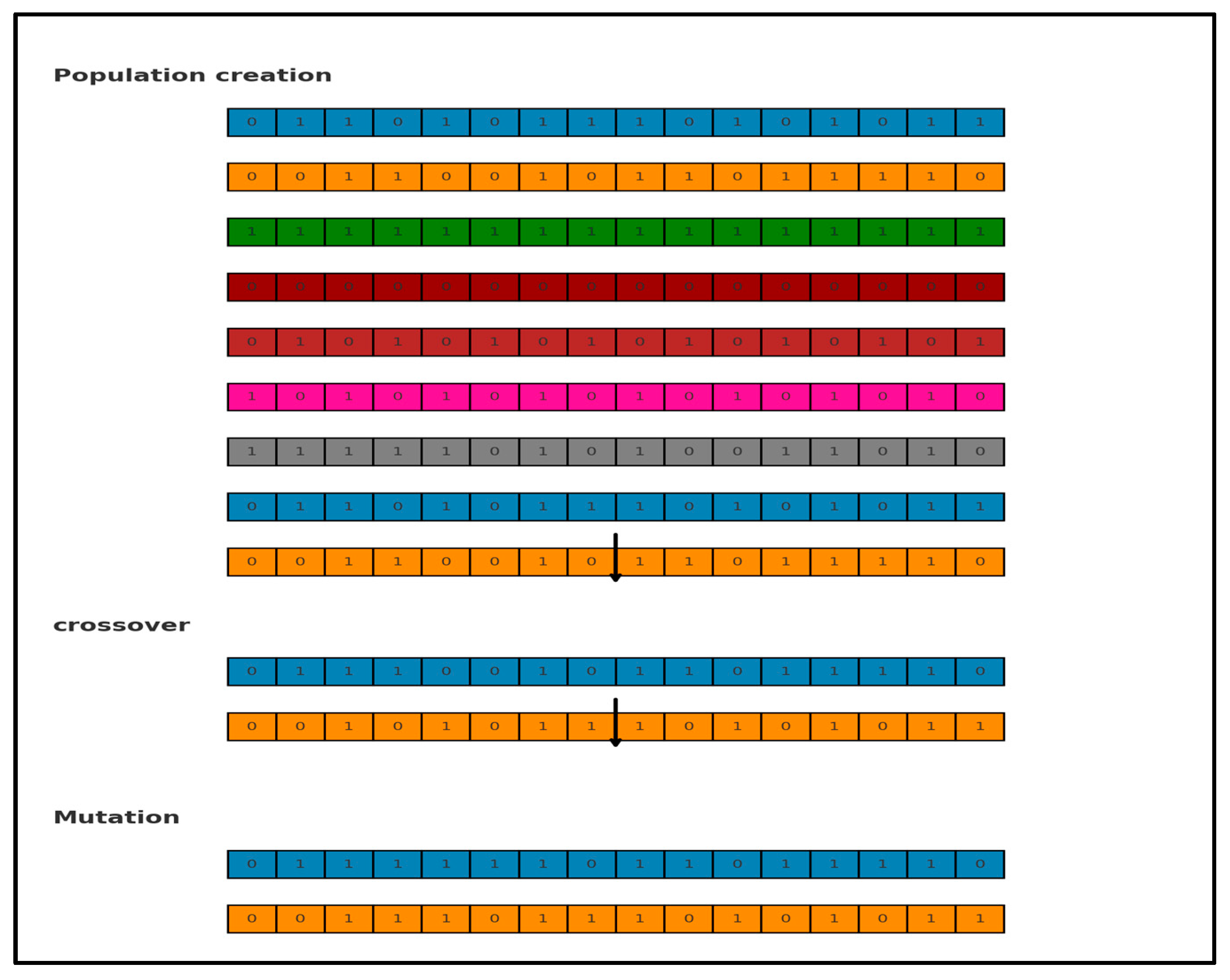
The genetic algorithm (GA) was utilised to extract key attributes from the time series dataset. As shown in Figure 5, the procedure began with the creation of an initial population composed of random candidates. These individuals were assessed through a fitness evaluation metric. Top-performing candidates were retained without alteration for the subsequent iteration, while the remaining members undergo recombination and modification operations to produce the next generation [29].
The dataset included 28 distinct parameters relevant to forecasting air temperature. To identify the most impactful ones, a binary encoding approach was applied, where sequence like [1, 0, 0, 1, 1, …] signified inclusion (1) or exclusion (0) of each parameter. Each sequence acted as a candidate solution, and each binary digit within it was termed a “gene”. These genes were initialised randomly. According to Figure 5, the number of genes was N = 12 with a population size of 8. Each candidate was scored using an evaluation criterion, with higher-scoring solutions advancing. Poorly performing candidates were discarded. Through genetic operations, namely crossover and mutation, a new generation of candidates was generated, as depicted in Figure 5.
Table 1 presents the GA parameters. As previously mentioned, selecting an optimal number of chromosomes was a crucial step in the evolutionary computation process. Existing research provided varying insights on the appropriate population size, with some studies indicating that a small population may lead to suboptimal solutions, while a larger population demands higher computational resources. To define a subset of features, a trapping function is utilised to assess the suitability of each subset. We adopted the {@(x) -var(X_all.* x, 0, ‘all’)} function as the fitness function. GA effectively minimised the error rate and selected individuals with the best fitness scores, thereby reducing the number of features. The prediction process evaluated the entire training dataset to identify the most similar K instances for generating new data points. Various population sizes were tested in this study to determine the optimal configuration.

2.2.3. LSTM

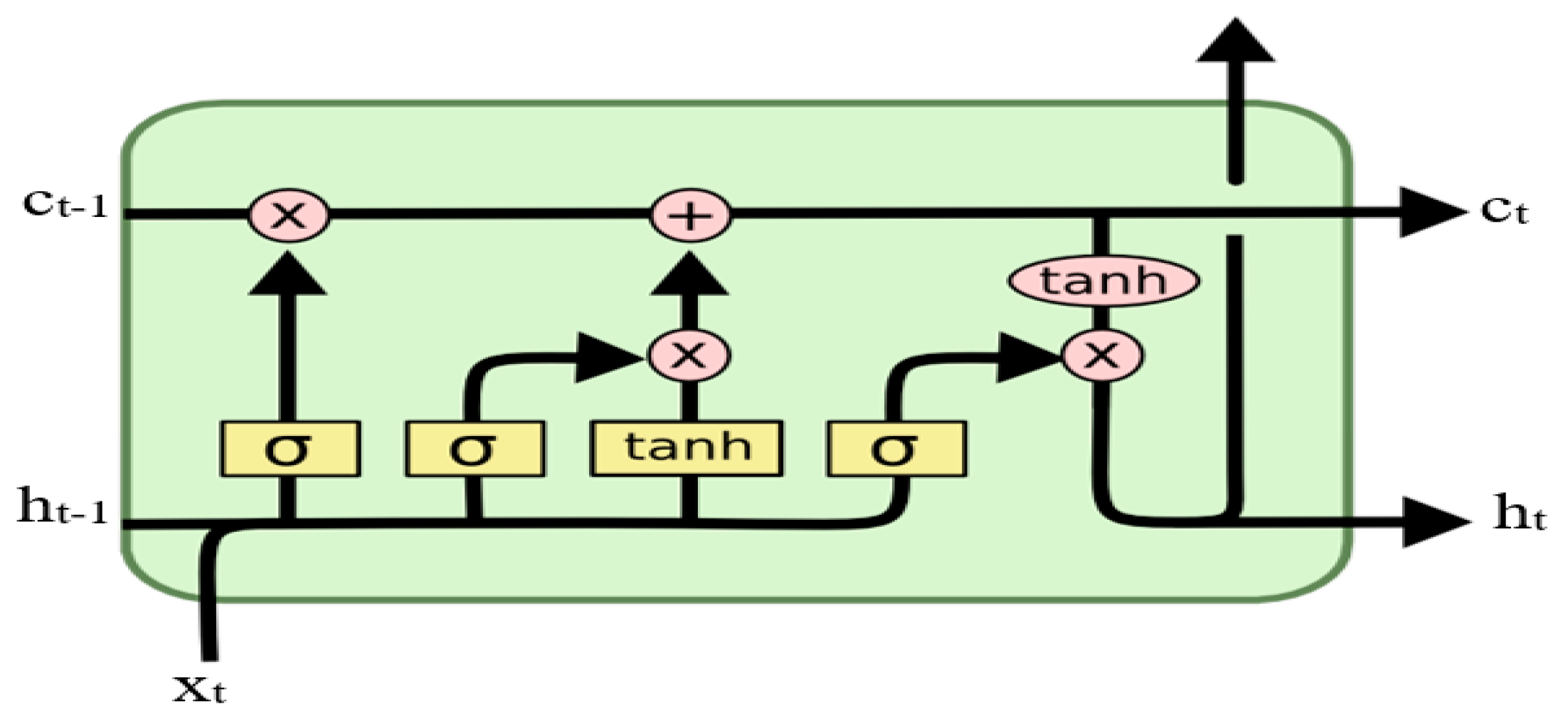
The architecture of LSTM is constructed as follows [30]: Within the memory block, there are one or more core cells that are self-connected to three multiplicative units known as the input, output, and forget gates. The presence of additional units in a system influences the transmission of information. Specifically, the multiplication of input values safeguards the memory block from disturbances caused by irrelevant inputs. Additionally, the output gates shield other units from obtaining irrelevant information pertaining to the current block [30,31]. The units function as gates to prevent weight conflicts. The input gate determines when to retain information or omit material within the block, and the output gate determines the timing of accessing the block and prevents interference with other blocks. At the time t, the inputs of the LSTM module contain the combined significant wave height representation x and the memory cell state c. At time t, the inputs of the LSTM module contain the combined significant wave height representation xt, the memory cell state ct−1, and the output of the LSTM module ht−1. yt denotes memory information. The LSTM computing process is as follows:
I t   = s i g W I   x t + U I h t 1 +   b I  
f t   = s i g W f   x t + U f h t 1 + b f  
o t   = s i g W o   x t + U o h t 1 + b o  
  y t   = t a n h W c   x t + U c h t 1 + b c  
c t = I t   c t 1 + f t y t    
h t   = o t t a n h ( c t )
where W and U denote weight matrices and b denotes bias vectors. Sig and tanh are smooth step functions and hyperbolic tangent functions. The output of the LSTM module ct and ht were the input of the LSTM module as shown in Figure 6.

2.2.4. Model Development

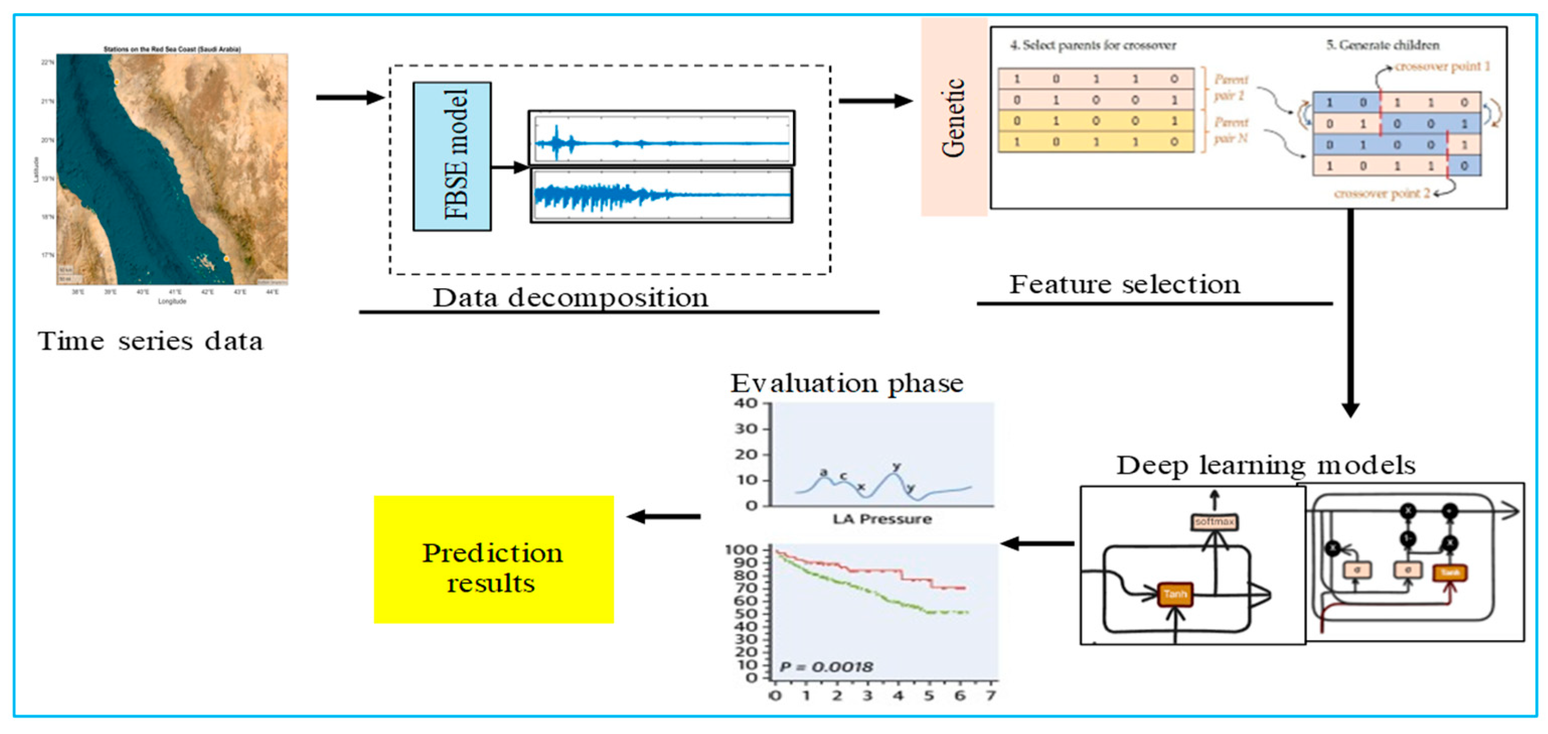
In this section, the model development is explained. To predict the daily, weekly, and monthly dry-bulb air temperature, we designed a hybrid architecture utilising the Fourier–Bessel series expansion (FBSE), a genetic algorithm (GA), and an LSTM. The time series data were passed through FBSE, then the GA was applied to extract the important features from the FBSE coefficients and reduce the dimensionality. Then, the outputs of the GA were sent to the GRU, BiGRU, LSTM, and BilSTM models [32,33,34].
The structure of the model designed for forecasting the dry-bulb air temperature is illustrated in Figure 7. The data were segmented into three subsets: training (60%), validation (20%), and testing (20%). Model fitting was carried out using the training subset. To monitor and evaluate performance during training, the validation data were utilised independently and excluded from the fitting phase. The validation loss served as the criterion for selecting the model’s optimal parameter configuration. No random sampling or shuffling was applied to avoid temporal information leakage. The FBSE decomposition was applied exclusively to the training data. The decomposition parameters obtained from the training set were then used to transform the validation and testing sets. This ensured that no information from the testing set was available during training, preserving the integrity and reproducibility of the prediction model.

3. Experimental Results

This section reports the results of the dry-bulb air temperature prediction based on the proposed model for the two regions in Saudia Arabia. This study evaluated the performance of the proposed model, which integrated FBSE, GA, and LSTM techniques to predict one-day, one-week, and one-month dry-bulb air temperatures. For the one-day-ahead prediction, we used the time series data from a single day (t − 1) as the input to forecast the next day (t). For the one-week-ahead prediction, we used the complete preceding week of the time series data (t − 7 to t − 1) to forecast the aggregated value for the following week. Similarly, for the one-month-ahead prediction, we used the preceding month of the time series data (t − 30 to t − 1) to predict the aggregated value for the following month. The dataset was segmented chronologically into 60% training, 20% validation, and 20% testing sets respectively. No random sampling was applied. The FBSE decomposition was applied exclusively to the training data.

3.1. Evaluation Metrics

The test set was utilised to evaluate the performance of the completed model. Several metrics were used to measure this performance, and Table 2 summarises all the metrics applied in the evaluation of the proposed model [35,36,37,38].

3.2. Benchmark Models

In this paper, the proposed FBSE-GA was hybridised with several benchmark models: GRU, BiGRU, LSTM, and BiLSTM. The following section provides a brief description of these models. Table 3 lists all the hyperparameters of the proposed models.
GRU: GRU was utilised as a foundational model to benchmark the performance of the hybrid approach for temperature prediction. A hybrid approach can significantly enhance the accuracy of dry-bulb air temperature predictions. This model can leverage various components.
BiGRU: Incorporating the bidirectional gated recurrent unit (BiGRU) effectively captures bidirectional dependencies within the data, leading to improved prediction accuracy.
BiLSTM: Employing bidirectional long short-term memory (BiLSTM) as an alternative to standard LSTM can reveal its advantages in recognising complex patterns within the dataset.
While the hybrid model harnesses the strengths of its components, it may demand substantial computational resources, especially when processing large datasets. Furthermore, the model’s performance can be sensitive to the choice of hyperparameters, requiring meticulous tuning and optimisation.
The complexity of the models and techniques involved may create challenges in interpreting results and understanding the underlying relationships within the data. By exploring the integration of FBSE with GRU, BiGRU, and BiLSTM in a hybrid framework, a more accurate and robust model for predicting the dry-bulb air temperature can be developed.

4. The Obtained Results

4.1. One-Day-Ahead Prediction Results

Table 4, the prediction results are listed for the two regions, Jazan and Jeddah; in terms of the regression ( R ) , RMSE, and MAE, a perfect predictor score is indicated by R values close to 1, while the ideal RMSE/MAE values are close to 0. In addition, with the metrics Willmott’s Index ( W I ), Nash–Sutcliffe Efficiency ( N S E ), and Legate–McCabe Efficiency ( L M E ), the accurate prediction model is expected to be close to 1, while the mean absolute percentage error ( M A P E ) and root mean square percentage error ( R M S P E ) should approach 0%.
From the results in Table 4, it was noted that the hybrid models FBSE-GA-BiLSTM, FBSE-GA-GRU, FBSE-GA-LSTM, and FBSE-GA-BiGRU showed superior prediction results compared to individual models. The FBSE-GA-LSTM scored the highest predictive accuracy with an R = 0.986, RMSE = 1.754, and MAE = 1.432, W I = 0.965 , N S E = 0.943 , M A P E = 7.200 , and M S P E = 8.786 for the Jeddah region, and R = 0.982, RMSE = 1.742, and MAE=1.410. W I = 0.954 , N S E = 0.933 , M A P E = 7.176 , and R M S P E = 8.732 for the Jazan region. The results indicated strong predictive abilities for the hybrid models compared with individual models. However, the LSTM showed high prediction results compared with other individual models GRU, BiGRU, and BiLSTM. Overall, the results indicated the superior performance of the FBSE-GA-LSTM and FBSE-GA-BiLSTM models compared to the other individual and hybrid models. The improved DBT prediction can be recognised in the FBSE-GA model which showed a strong resistance to noise.
The results for the two regions, Jazan and Jeddah, demonstrated that the hybrid models delivered the highest performances as shown in Table 4, with the lowest RMSE at 1.754 and 1.773 and a MAE of 1.432 and 1.465 recorded for FBSE-GA-LSTM and FBSE-GA-BiLSTM, respectively, proving that the proposed model closely corresponding observed values.
All hybrid models coupled with the FBSE-GA model demonstrated higher performance; for example, FBSE-GA-LSTM and FBSE-GA-BiLSTM achieved the second and the highest prediction rates in terms of W I and N S E . Figure 8 reports the results in terms of LME. It can be noted that all hybrid models outperformed individual models, with LME values ranging from 0.901 to 0.912, significantly improving the performance of LSTM, GRU, BiLSTM, and BiGRU models. These results confirmed the effectiveness of integrating LSTM, GRU, BiLSTM, and BiGRU models with FBSE-GA in enhancing model accuracy. In addition, the persistence model showed a high performance compared to deep learning models.

4.2. One-Week-Ahead Prediction

In this experiment, hybrid models were tested one week before the prediction of DBT. From the results obtained in Table 5, it was observed that all hybrid models outperformed individual models with the FBSE-GA-LSTM model scoring the highest prediction with R = 0.975, and an RMSE = 1.778 showed a high correlation with observed values. This high correlation proved the proposed FBSE-GA was effective in accurately replicating weekly DBT prediction in both regions.
Table 5 reports the one-week-ahead prediction rates for the Jazan region, and these findings confirmed that integrating the LSTM, GRU, BiLSTM, and BiGRU models with FBSE-GA improved their prediction accuracy and surpassed standalone approaches. Furthermore, all hybrid (FBSE-GA-LSTM, FBSE-GA-GRU, FBSE-GA-BiLSTM, and FBSE-GA-BiGRU) models demonstrated consistent precision rates for one week ahead and their MAPE values were under 8%. The obtained results indicated that hybridisation improved the predictive accuracy of LSTM, GRU, BiLSTM, and BiGRU compared to their standalone performance. It was noted that the persistence model kept showing a good performance in the one-week prediction and delivered consistently low prediction errors.
The performance of all hybrid models was evaluated in term of LME. From the results in Figure 9, hybrid models showed their superior performances, with FBSE-GA-LSTM and FBSE-GA-BiLSTM scoring the highest values of 0.9337 and 0.903, respectively.
The comparative analysis revealed that the proposed FBSE-GA model improved the performance of all models, with an increase in R ranging 7–9%. The best hybrid model was the FBSE-GA-LSTM, which showed its superior ability to predict the weekly dry-bulb air temperature. Moreover, the FBSE-GA-BiLSTM recorded the lowest RMSE.

4.3. One-Month-Ahead Prediction Results

The proposed hybrid model FBSE-GA-BiLSTM was evaluated to predict the one-month-ahead dry-bulb air temperature. As shown in Table 6, all hybrid models outperformed when compared to the individual models. Specifically, the FBSE-GA-BiLSTM model achieved the highest R of 0.954, with an RMSE of 1.780. This highest R indicated that the proposed FBSE-GA-BiLSTM model effectively reproduces the monthly-ahead DBT in the two regions, Jazan and Jeddah.
In addition, the FBSE-GA-LSTM scored the second-highest prediction rate compared to the other hybrid models, FBSE-GRU and FBSE-BiGRU.
A further assessment was carried out using the LME metric, as shown in Figure 10, which demonstrated that the FBSE-GA-BiLSTM model scored the highest prediction rates of 0.903, 0.8337, and 0.893, respectively. These results proved that combining the models into hybrid (FBSE-GA-BiLSTM, FBSE-GA-LSTM, FBSE-GA-GRU, FBSE-GA-BiGRU) models surpasses standalone models. Additionally, based on the MAPE metric, all hybrid models (FBSE-GA-BiLSTM, FBSE-GA-LSTM, FBSE-GA-GRU, FBSE-GA-BiGRU) recoded lower MAPE values <10%. These results support the superior predictive output of hybrid models over individual models.
Across all experiments, the proposed FBSE-GA-BiLSTM model scored the highest prediction rate for the one-day, one-month, one-week predictions. These findings indicated that the proposed FBSE-GA model effectively improved the performance of deep learning models.

5. Discussion

The findings highlight the importance of integrating the decomposition model with deep learning architectures for achieving accurate predictions. The article “Hybrid Model of Feature-Based Selection and Extraction and Genetic Algorithms GA for Optimizing the Prediction of Complex and Non-Stationary Time Series” was submitted for hybrid models to predict nonstationary and complex time series data, which extended the concept of hybrid models by integrating feature-based selection and extraction (FBSE) and genetic algorithms (GA), that optimised model parameters, performed data decomposition with selected features, and eliminated the abnormal values of selecting features. This complementary relationship enabled us to seek out significant patterns from complex data and to optimise model parameters for accurate forecast. Combining these methods enabled us to handle the difficulty of nonlinearity, non-stationarity, and noise in time series data, thus improving the prediction accuracy. In addition, the FBSE-based GA demonstrated a strong performance in analysing the nonstationary and complex time series data. The relationship between the novelty of the decomposition model, feature selection, and deep learning models became clear in cases where the datasets did not necessarily satisfy the independent and identically distributed requirement. In our work to tackle these problems in DBT prediction, we introduced a hybrid model of FBSE, GA, and BiLSTM. The main discovery is described in this section.
1.
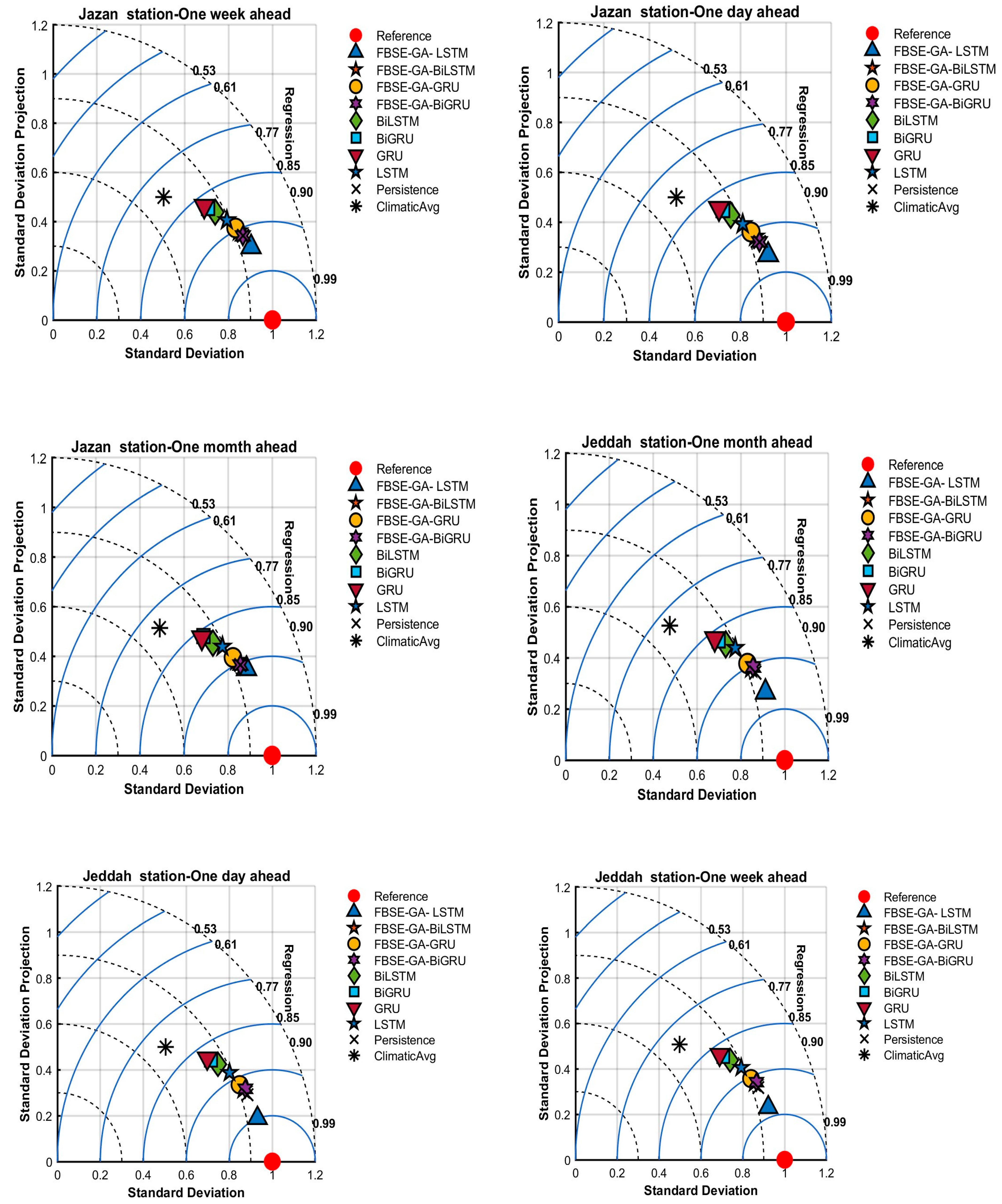
Figure 11 reports the results using Taylor diagrams. From the results, we can observe that all hybrid models were close to actual values. The proposed FBSE-GA coupled with LSTM, GRU, BiLSTM, and BiGRU models scored the highest R values for the two (Jeddah and Jazan) stations. The values generated by the individual LSTM, GRU, BiLSTM, and BiGRU models differed significantly from those generated by the actual model. For weekly and monthly air temperature predictions, it can be observed the proposed FBSE-GA-LSTM outperformed all hybrid and individual models.
2.
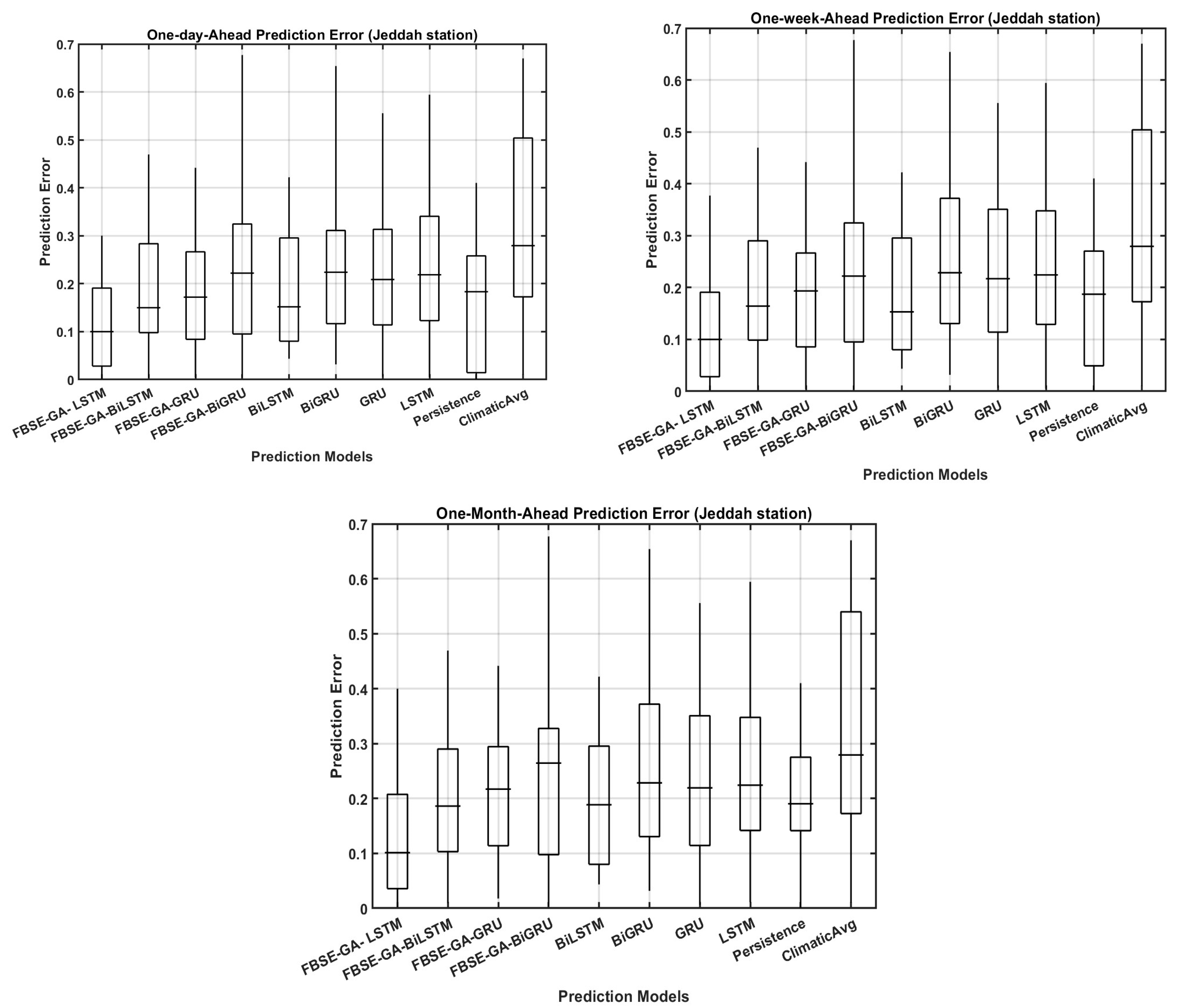
Figure 12 reports the prediction error (FE) boxplots for the daily, weekly, and monthly dry-bulb air temperature predictions for all hybrid models using the Jazan station data. The results revealed that with monthly dry-bulb air temperature prediction, all models exhibited low error forecasting accuracy across the two regions compared to the daily and weekly predictions. For the daily prediction, all hybrid models showed lower FE, while the individual models exhibited high FE. These findings indicated the ability of integrating FBSE-GA with deep learning models to improve dry-bulb air temperature prediction.
3.
To validate the efficiency of the proposed model, FBSE-GA-LSTM, it was compared with the classic decomposition models fast Fourier transform (FFT) and discrete wavelet transform (DWT). Comparisons with DWT and Fourier transform (FF) were also conducted. In this experiment, FFT and DWT were integrated with GA and LSTM for fair comparison. Table 7 reports the comparison results. It was observed that FBSE outperformed FFT and DWT in terms of R and WI. In addition, the FBSE was faster, and utilised less computation time compared with FFT and DWT.
4.
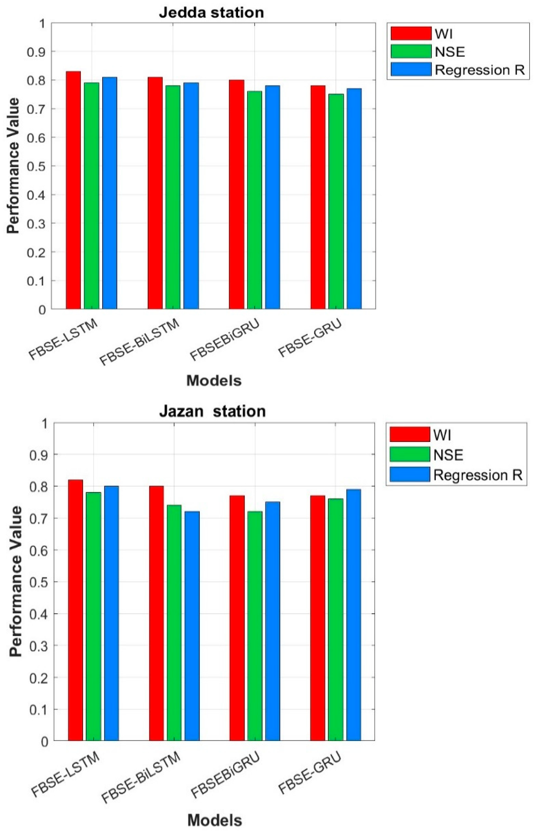
This study also examined the effect of GA on the prediction rate. Figure 13 shows the performance of all hybrid models without GA. The FBSE coefficients were sent directly to all models without GA. The results showed that all models’ performance was degraded and poor. The results confirmed that the combination of FBSE and GA improved the predictive accuracy of all models.
5.
The computational cost of the proposed FBSE-GA-LSTM and the state-of-the-art models were evaluated in terms of complexity time. Based on the results, the statistical model’s persistence and climatic average scored the lowest computational times, with training times below 16 s, reflecting their simplicity and absence of model parameter optimisation. In contrast, most of the deep learning models, particularly the proposed models, exhibited longer training times due to the additional cost associated with the GA-based feature selection phase. For example, FBSE-GA-LSTM scored approximately 320 s to train, compared to 180 s for the LSTM, exhibiting the added optimisation overhead. Overall, these results demonstrated that the proposed models offer a favourable trade-off between improved accuracy and acceptable computational overhead, especially in applications where training is performed offline, as shown in Figure 14.
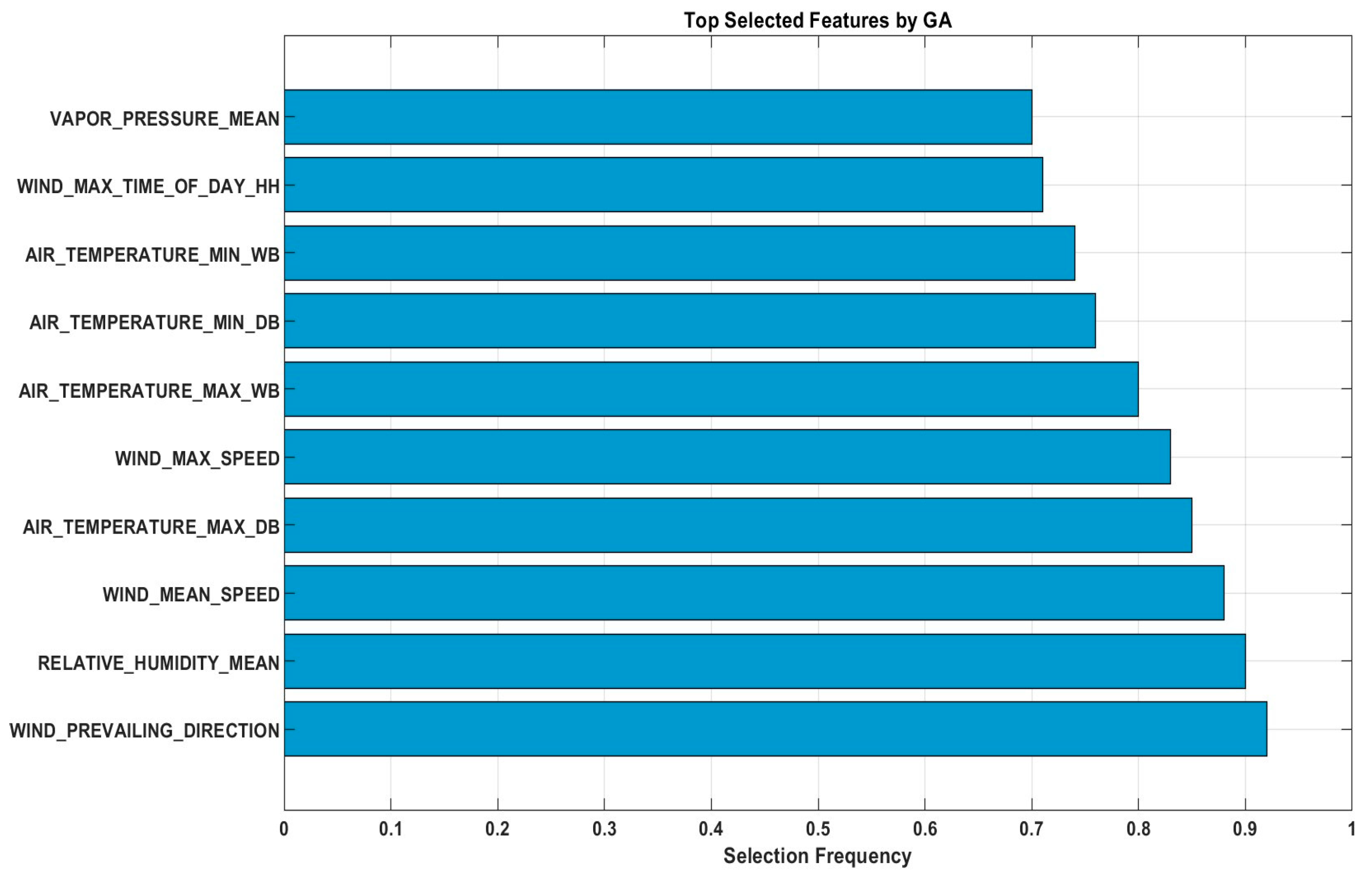
To enhance the interpretability of the proposed model, we conducted a feature analysis to show which features were selected by the GA across 100 optimisation runs. The results showed that WIND_MEAN_SPEED, RELATIVE_HUMIDITY_MEAN, AIR_TEMPERATURE_MAX_DB, WIND_PREVAILING_DIRECTION, WIND_MAX_SPEED, AIR_TEMPERATURE_MAX_WB, AIR_TEMPERATURE_MIN_DB, AIR_TEMPERATURE_MIN_W, WIND_MAX_TIME_OF_DAY_HH, and VAPOR_PRESSURE_MEAN were the top ten features, each with a selection frequency exceeding 75%. Based on our findings these features capture influential meteorological conditions influencing temperature dynamics, such as wind patterns, humidity, and temperature extremes. Figure 15 presents a bar chart of the selection frequencies, which demonstrated that the GA effectively identifies the most relevant inputs, thereby enhancing model efficiency and reducing redundancy without compromising predictive performance. The feature wind direction had the most significant influence on DBT because it directly affects heat advection and air mass movement in the study area. Certain wind directions are associated with the transport of warmer or cooler air masses, which can substantially alter the local dry-bulb temperature. This relationship reflects the climatological patterns of the region, where prevailing winds often coincide with the specific thermal characteristics of incoming air.
The integration of decomposition models with deep learning architectures has shown promise in enhancing the predictive accuracy of hybrid models for nonstationary and complex time series data. Nevertheless, there are still restrictions, and future prospects should be considered to achieve more perfection on these models. The challenges are largely related to the integration of models, computational constraints, and the handling of more diverse datasets. The work presented here could be extended to better models for such issues and other approaches for better accuracy and performance. One of our future works is that the proposed model will be applied to predict other variables such as the relative humidity and wind speed as it was designed to work on multivariate time series data.

6. Conclusions

In this study, an accurate model of FBSE, GA, and BiLSTM was developed for predicting the DBT, indicating the extraordinary precision of these models to predict temperature fluctuation. Using hybrid techniques, the research assured that the predictive quality was enhanced by combining FBSE-GA with LSTM rather than the separated models. The results highlighted the importance of GA in choosing the essential features for enhancing the model robustness. Results also showed that the predictive accuracy of hybrid models was superior in the case of the changing seasonality.
While the proposed model showed high performance against the standard models, this study did not include comparisons with established regional or numerical weather prediction (NWP) models for temperature forecasting. Such models, which include broader atmospheric dynamics and regional climate data, could improve the evaluation phase of the paper. Including these comparisons in future work would help contextualise the results within the wider environment of temperature prediction models.

Author Contributions

Conceptualisation, H.A., M.A. and M.D.; methodology, H.A., M.A. and M.D.; validation, H.A.; formal analysis, H.A., M.A. and M.D.; investigation, H.A., M.A., M.D. and A.A.A.; resources, A.A.A.; data curation, H.A. and M.A.; writing—original draft preparation, H.A. and M.A.; writing—review and editing, A.A.A., M.A., R.C.D., A.A.F. and S.A.; visualisation, H.A.; supervision, M.A., A.A.A., R.C.D. and A.A.F.; All authors have read and agreed to the published version of the manuscript.

Funding

This work was funded by the Deanship of Scientific Research, Vice Presidency for Graduate Studies and Scientific Research, King Faisal University, Saudi Arabia [Project No. KFU253051].

Data Availability Statement

The authors do not have the permission to share the data.

Acknowledgments

The authors are thankful to the Department of Meteorology, Saudi Arabia for providing the relevant datasets.

Conflicts of Interest

The authors declare that they have no known competing financial interests or personal relationships that could have appeared to influence the work reported in this paper.

References

  1. Liljegren, J.C.; Carhart, R.A.; Lawday, P.; Tschopp, S.; Sharp, R. Modeling the wet bulb globe temperature using standard meteorological measurements. J. Occup. Environ. Hyg. 2008, 5, 645–655. [Google Scholar] [CrossRef]
  2. Yang, R.; Hu, J.; Li, Z.; Mu, J.; Yu, T.; Xia, J.; Li, X.; Dasgupta, A.; Xiong, H. Interpretable machine learning for weather and climate prediction: A review. Atmos. Environ. 2024, 338, 120797. [Google Scholar] [CrossRef]
  3. Apaydin, M.; Yumuş, M.; Değirmenci, A.; Karal, Ö. Evaluation of air temperature with machine learning regression methods using Seoul City meteorological data. Pamukkale Univ. J. Eng. Sci. 2022, 28, 737–747. [Google Scholar] [CrossRef]
  4. Palmer, T.N. A nonlinear dynamical perspective on model error: A proposal for non-local stochastic-dynamic parametrization in weather and climate prediction models. Q. J. R. Meteorol. Soc. 2001, 127, 279–304. [Google Scholar] [CrossRef]
  5. Adnan, R.M.; Liang, Z.; Kuriqi, A.; Kisi, O.; Malik, A.; Li, B.; Mortazavizadeh, F. Air temperature prediction using different machine learning models. Indones. J. Electr. Eng. Comput. Sci. 2021, 22, 534–541. [Google Scholar] [CrossRef]
  6. Ali, M.; Prasad, R. Significant wave height forecasting via an extreme learning machine model integrated with improved complete ensemble empirical mode decomposition. Renew. Sustain. Energy Rev. 2019, 104, 281–295. [Google Scholar] [CrossRef]
  7. Gündoğdu, S.; Elbir, T. Application of feed forward and cascade forward neural network models for prediction of hourly ambient air temperature based on MERRA-2 reanalysis data in a coastal area of Turkey. Meteorol. Atmos. Phys. 2021, 133, 1481–1493. [Google Scholar] [CrossRef]
  8. Tehrani, A.A.; Veisi, O.; Delavar, Y.; Bahrami, S.; Sobhaninia, S.; Mehan, A. Predicting urban Heat Island in European cities: A comparative study of GRU, DNN, and ANN models using urban morphological variables. Urban Clim. 2024, 56, 102061. [Google Scholar] [CrossRef]
  9. Hasan, M.M.; Hasan, M.J.; Rahman, P.B. Comparison of RNN-LSTM, TFDF and stacking model approach for weather forecasting in Bangladesh using historical data from 1963 to 2022. PLoS ONE 2024, 19, e0310446. [Google Scholar] [CrossRef]
  10. Huang, C.; He, W.; Liu, J.; Nguyen, N.T.; Yang, H.; Lv, Y.; Chen, H.; Zhao, M. Exploring the Potential of Long Short-Term Memory Networks for Predicting Net CO2 Exchange Across Various Ecosystems ss Multi-Source Data. Authorea Prepr. 2023. [Google Scholar] [CrossRef]
  11. Gong, B.; Langguth, M.; Ji, Y.; Mozaffari, A.; Stadtler, S.; Mache, K.; Schultz, M.G. Temperature forecasting by deep learning methods. Geosci. Model Dev. 2022, 15, 8931–8956. [Google Scholar] [CrossRef]
  12. Feng, Z.; Zhang, D.; Zuo, M.J. Adaptive mode decomposition methods and their applications in signal analysis for machinery fault diagnosis: A review with examples. IEEE Access 2017, 5, 24301–24331. [Google Scholar] [CrossRef]
  13. Wu, Z.; Huang, N.E. Ensemble empirical mode decomposition: A noise-assisted data analysis method. Adv. Adapt. Data Anal. 2009, 1, 1–41. [Google Scholar] [CrossRef]
  14. Colominas, M.A.; Schlotthauer, G.; Torres, M.E. Improved complete ensemble EMD: A suitable tool for biomedical signal processing. Biomed. Signal Process. Control 2014, 14, 19–29. [Google Scholar] [CrossRef]
  15. Hadi, S.J.; Tombul, M. Streamflow forecasting using four wavelet transformation combinations approaches with data-driven models: A comparative study. Water Resour. Manag. 2018, 32, 4661–4679. [Google Scholar] [CrossRef]
  16. Liu, W.; Liu, Y.; Li, S.; Chen, Y. A review of variational mode decomposition in seismic data analysis. Surv. Geophys. 2023, 44, 323–355. [Google Scholar] [CrossRef]
  17. Bagri, I.; Tahiry, K.; Hraiba, A.; Touil, A.; Mousrij, A. Vibration Signal Analysis for Intelligent Rotating Machinery Diagnosis and Prognosis: A Comprehensive Systematic Literature Review. Vibration 2024, 7, 1013–1062. [Google Scholar] [CrossRef]
  18. Rehman, N.; Mandic, D.P. Multivariate empirical mode decomposition. Proc. R. Soc. A Math. Phys. Eng. Sci. 2010, 466, 1291–1302. [Google Scholar] [CrossRef]
  19. Tang, M.; Sheng, W.; Qiu, J.; Zhang, C.; Li, H. Short-term load forecasting of electric vehicle charging stations based on adaptive VMD-BiLSTM. J. Ind. Manag. Optim. 2025, 21, 2107–2129. [Google Scholar] [CrossRef]
  20. Ahmed, A.A.; Deo, R.C.; Ghahramani, A.; Feng, Q.; Raj, N.; Yin, Z.; Yang, L. New double decomposition deep learning methods for stream-flow water level forecasting using remote sensing modis satellite variables, climate indices and observations. Sci. Total Environ. 2022, 831, 154722. [Google Scholar] [CrossRef]
  21. Bhattacharyya, A.; Pachori, R.B. A multivariate approach for patient-specific EEG seizure detection using empirical wavelet transform. IEEE Trans. Biomed. Eng. 2017, 64, 2003–2015. [Google Scholar] [CrossRef]
  22. Duan, W.Y.; Han, Y.; Huang, L.M.; Zhao, B.B.; Wang, M.H. A hybrid EMD-SVR model for the short-term prediction of significant wave height. Ocean. Eng. 2016, 124, 54–73. [Google Scholar] [CrossRef]
  23. Zhou, J.; Wang, D.; Band, S.S.; Mirzania, E.; Roshni, T. Atmosphere air temperature forecasting using the honey badger optimization algorithm: On the warmest and coldest areas of the world. Eng. Appl. Comput. Fluid Mech. 2023, 17, 2174189. [Google Scholar] [CrossRef]
  24. Hou, J.; Wang, Y.; Zhou, J.; Tian, Q. Prediction of hourly air temperature based on CNN–LSTM. Geomat. Nat. Hazards Risk 2022, 13, 1962–1986. [Google Scholar] [CrossRef]
  25. Mohammed, H.; Diykh, M. Improving EEG major depression disorder classification using FBSE coupled with domain adaptation method-based machine learning algorithms. Biomed. Signal Process. Control 2023, 85, 104923. [Google Scholar] [CrossRef]
  26. Fister, D.; Pérez-Aracil, J.; Peláez-Rodríguez, C.; Del Ser, J.; Salcedo-Sanz, S. Accurate long-term air temperature prediction with Machine Learning models and data reduction techniques. Appl. Soft Comput. 2023, 136, 110118. [Google Scholar] [CrossRef]
  27. Diykh, M.; Ali, M.; Labban, A.H.; Prasad, R.; Jamei, M.; Abdulla, S.; Farooque, A.A. Designing empirical fourier decomposition reinforced with multiscale increment entropy and deep learning to forecast dry bulb air temperature. Results Eng. 2025, 26, 104597. [Google Scholar] [CrossRef]
  28. Dash, S.; Ghosh, S.K.; Tripathy, R.K.; Panda, G.; Pachori, R.B. Fourier-Bessel domain based discrete Stockwell transform for the analysis of non-stationary signals. In Proceedings of the 2022 IEEE India Council International Subsections Conference (INDISCON), Bhubaneswar, India, 15–17 July 2022; pp. 1–6. [Google Scholar]
  29. Diykh, M.; Abdulla, S.; Deo, R.C.; Siuly, S.; Ali, M. Developing a novel hybrid method based on dispersion entropy and adaptive boosting algorithm for human activity recognition. Comput. Methods Programs Biomed. 2023, 229, 107305. [Google Scholar] [CrossRef]
  30. Hochreiter, S.; Schmidhuber, J. Long short-term memory. Neural Comput. 1997, 9, 1735–1780. [Google Scholar] [CrossRef] [PubMed]
  31. Yu, Y.; Si, X.; Hu, C.; Zhang, J. A review of recurrent neural networks: LSTM cells and network architectures. Neural Comput. 2019, 31, 1235–1270. [Google Scholar] [CrossRef] [PubMed]
  32. Nosouhian, S.; Nosouhian, F.; Khoshouei, A.K. A review of recurrent neural network architecture for sequence learning: Comparison between LSTM and GRU. Preprints 2021. [Google Scholar] [CrossRef]
  33. She, D.; Jia, M. A BiGRU method for remaining useful life prediction of machinery. Measurement 2021, 167, 108277. [Google Scholar] [CrossRef]
  34. Al-Saadi, Y.R.; Tapou, M.S.; Badi, A.A.; Abdulla, S.; Diykh, M. Developing smart self orienting solar tracker for mobile PV power generation systems. IEEE Access 2022, 10, 79090–79099. [Google Scholar] [CrossRef]
  35. Faris, N.; Sahi, A.; Diykh, M.; Abdulla, S.; Siuly, S. Enhanced Polycystic Ovary Syndrome diagnosis model leveraging a K-means based genetic algorithm and ensemble approach. Intell.-Based Med. 2025, 11, 100253. [Google Scholar] [CrossRef]
  36. Diykh, M.; Ali, M.; Jamei, M.; Abdulla, S.; Uddin, M.P.; Farooque, A.A.; Labban, A.H.; Alabdally, H. Empirical curvelet transform based deep DenseNet model to predict NDVI using RGB drone imagery data. Comput. Electron. Agric. 2024, 221, 108964. [Google Scholar] [CrossRef]
  37. Kazemi, S.M.; Saffarian, M.; Babaiyan, V. Time series forecasting of air temperature using an intelligent hybrid model of genetic algorithm and neural network. J. Ind. Syst. Eng. 2021, 13, 1–15. [Google Scholar]
  38. Yaprakdal, F.; Varol Arısoy, M. A multivariate time series analysis of electrical load forecasting based on a hybrid feature selection approach and explainable deep learning. Appl. Sci. 2023, 13, 12946. [Google Scholar] [CrossRef]
Figure 1. Map of the study locations in Saudi Arabia where the proposed FBSE-GA-LSTM hybrid model was implemented.
Forecasting 07 00046 g001
Figure 2. Descriptive analysis of the normalised data collected from the Jeddah and Jazan stations used to evaluate the efficacy of the proposed FBSE-GA-LSTM hybrid model.
Forecasting 07 00046 g002
Figure 3. Basis function plot (a) with FFT coefficients and (b) with BF coefficients.
Forecasting 07 00046 g003
Figure 4. The FBSE coefficients for the different variables of Jazan station.
Forecasting 07 00046 g004
Figure 5. The main process of GA.
Forecasting 07 00046 g005
Figure 6. The structure of the LSTM.
Forecasting 07 00046 g006
Figure 7. Proposed model for dry-bulb air temperature prediction.
Forecasting 07 00046 g007
Figure 8. LME of each model for one-day ahead prediction in both stations.
Forecasting 07 00046 g008
Figure 9. LME for the weekly performance evaluation of each model.
Forecasting 07 00046 g009
Figure 10. LME for the monthly performance evaluation.
Forecasting 07 00046 g010
Figure 11. Tayler plots for Jeddah and Jazan stations.
Forecasting 07 00046 g011
Figure 12. Boxplots for Jeddah and Jazan stations.
Forecasting 07 00046 g012
Figure 13. Performance evaluation without GA for Jeddah and Jazan stations.
Forecasting 07 00046 g013
Figure 14. Training time for each model.
Forecasting 07 00046 g014
Figure 15. Top selected features by GA.
Forecasting 07 00046 g015
Table 1. Genetic algorithm configuration settings.
ParameterValue
Total Features Considered27
Size of the Population30
Genome Length27
Population RepresentationdoubleVector
Fitness Function@(x) -var(X_all.* x, 0, ‘all’)
Number of generations20
Crossover Mechanismcrossoverscattered
Crossover Probability (CP)0.5 default
Mutation Strategymutationadaptfeasible
Mutation RateAdaptive (auto)
Selection Strategyselectionstochunif
Number of Elites Retainedceil(0.05 * PopulationSize) → 2
Table 2. Statistical performance metrics used in this paper.
MetricsEquations
Mean absolute error (MAE) M A E = m e a n ( i A t e s t i n g s e t | T a i r i T a i r i ¯ | )
Correlation coefficient (CORR) C O R R = 1 S P I t e s t i t e s t i n g _ s e t i ( T a i r i m e a n T a i r i ) ( T a i r i ¯ m e a n T a i r i ¯ ) ) i ( T a i r i m e a n T a i r i ) 2 i = 1 n T a i r i ¯ m e a n T a i r i ¯ ) 2
Willmott’s index (WI) W I = 1 i t e s t i n g s e t N ( T a i r i ¯ T a i r i ) 2 i t e s t i n g s e t N ( | T a i r i ¯ T a i r i + T a i r i ¯ T a i r i 2
Root square error (RSE) R S E = 1 i t e s t i n g s e t N ( T a i r i ¯ T a i r i ) 2 i t e s t i n g s e t N ( T a i r i ¯ T a i r i ) 2
Legates and McCabe’s index (LM) L M = 1 i t e s t i n g s e t N T a i r i ¯ T a i r i i t e s t i n g s e t N T a i r i ¯ T a i r i
Relative percentage error (RPE) R P E = 1 N t e s t i n g _ s e t N | T a i r i ¯ T a i r i T a i r i | × 100
Where T a i r i denotes the actual values and T a i r i ¯ refers to the predicted air temperature values. Low MAE and RSE values indicate a high performance.
Table 3. Hyperparameters of all models used for dry-bulb air temperature prediction.
ModelParameters
JeddahJazan
FBSE-GA-LSTMR = 1, alpha = 1, N = 200, PS = 20; MG = 100; MP = 0.1, ER = 0.01, CP = 0.5, PP = 0.3, CT = uniform’, dropout = 0.3, learning rate = 0.001–0.005, batch size = 64, epoch = 200.R = 1, alpha = 1, N = 200, PS = 30; MG = 100; MP = 0.1, ER = 0.01, CP = 0.5, PP = 0.3, CT = uniform’, dropout = 0.2, learning rate = 0.001–0.005, batch size = 64, epoch = 100.
FBSE-GA-BiLSTMR = 1, alpha = 1, N = 200, PS = 30; MG = 100; MP = 0.1, ER = 0.01, CP = 0.5, PP = 0.3, CT = uniform’, dropout = 0.3, learning rate = 0.001–0.005, batch size = 64, epoch = 200.R = 1, alpha = 1, N = 200, PS = 30; MG = 100; MP = 0.1, ER = 0.01, CP = 0.5, PP = 0.3, CT = uniform’, dropout = 0.2, learning rate = 0.001–0.005, batch size = 64, epoch = 100.
FBSE-GA-GRUR = 1, alpha = 1, N = 200, PS = 30; MG = 100; MP = 0.1, ER = 0.01, CP = 0.5, PP = 0.3, CT = uniform’, dropout = 0.3, learning rate = 0.001–0.005, batch size = 64, epoch = 200.R = 1, alpha = 1, N = 200, PS = 30; MG = 100; MP = 0.1, ER = 0.01, CP = 0.5, PP = 0.3, CT = uniform’, dropout = 0.2, learning rate = 0.001–0.005, batch size = 64, epoch = 100.
FBSE-GA-BiGRUR = 1, alpha = 1, N = 200, PS = 30; MG = 100; MP = 0.1, ER = 0.01, CP = 0.5, PP = 0.3, CT = uniform’, dropout = 0.3, learning rate = 0.001–0.005, batch size = 64, epoch = 200.R = 1, alpha = 1, N = 200, PS = 30; MG = 100; MP = 0.1, ER = 0.01, CP = 0.5, PP = 0.3, CT = uniform’, dropout = 0.2, learning rate = 0.001–0.005, batch size = 64, epoch = 100.
BiLSTMR = 1, alpha = 1, N = 200, dropout = 0.3, learning rate = 0.001–0.005, batch size = 64, epoch = 200.R = 1, alpha = 1, N = 200, dropout = 0.2, learning rate = 0.001–0.005, batch size = 64, epoch = 100.
BiGRUR = 1, alpha = 1, N = 200, dropout = 0.3, learning rate = 0.001–0.005, batch size = 64, epoch = 200.R = 1, alpha = 1, N = 200, dropout = 0.2, learning rate = 0.001–0.005, batch size = 64, epoch = 100.
GRUR = 1, alpha = 1, N = 200, dropout = 0.4, learning rate = 0.001–0.003, batch size = 64, epoch = 150.R = 1, alpha = 1, N = 200, dropout = 0.3, learning rate = 0.001–0.003, batch size = 64, epoch = 100.
LSTMR = 1, alpha = 1, N = 200, dropout = 0.3, learning rate = 0.001–0.005, batch size = 32, epoch = 200.R = 1, alpha = 1, N = 200, dropout = 0.2, learning rate = 0.001–0.005, batch size = 64, epoch = 200.
PersistenceTemporal split = Chronological (no shuffling)Temporal split = Chronological (no shuffling)
Climatic AvgTemporal split = Chronological (no shuffling)Temporal split = Chronological (no shuffling)
Upper limit of interval (R), number of coefficients (N), population size (PS), max generations (MG), mutation probability (MP), elitism ratio (ER), crossover probability (CP), parents portion (PP), crossover type (CT).
Table 4. One-day-ahead prediction results for Jazan and Jeddah stations.
Jazan Stations
Models R RMSEMAE W I N S E M A P E R M S P E
FBSE-GA-LSTM0.9861.7541.4320.9650.9437.2008.786
FBSE-GA-BiLSTM0.9541.7731.4650.9610.9427.2008.791
FBSE-GA-GRU0.9431.8641.4720.9530.9387.6008.793
FBSE-GA-BiGRU0.95218681.5120.9510.9367.6108.995
BiLSTM0.8762.2821.8420.8530.87410.239.772
BiGRU0.8542.8871.8630.8510.87310.259.781
GRU0.8432.9211.8780.8490.86310.289.792
LSTM0.9012.1231.7820.8640.88210.299.632
Persistence0.9471.7661.4220.7690.8217.188.811
ClimaticAvg0.7283.2111.9320.4780.59210.529.975
Jeddah Station
Models R RMSEMAE W I N S E M A P E R M S P E
FBSE-GA-LSTM0.9821.7421.4100.9540.9337.1768.732
FBSE-GA-BiLSTM0.9461.7711.4560.9510.9317.1828.681
FBSE-GA-GRU0.9381.8681.4790.9420.9317.7008.892
FBSE-GA-BiGRU0.94818691.5370.9480.9247.7708.999
BiLSTM0.8722.2841.8460.8500.87110.539.777
BiGRU0.8522.8811.8640.8430.86310.569.787
GRU0.8412.9201.8760.8370.83410.379.798
LSTM0.9002.1251.7860.8520.87710.339.633
Persistence0.9451.7631.4320.7620.8207.178.812
ClimaticAvg0.7193.2001.9530.4750.59110.519.976
Table 5. Prediction results based on different evaluation metrics (one week ahead) for Jazan and Jeddah stations.
Jazan Station
Models R RMSEMAE W I N S E M A P E R M S P E
FBSE-GA-LSTM0.9751.7781.4530.9540.9377.3008.794
FBSE-GA-BiLSTM0.9651.7791.4570.9550.9387.3018.797
FBSE-GA-GRU0.9631.7791.4540.9550.9387.3048.798
FBSE-GA-BiGRU0.9541.7811.4640.9430.9397.3088.799
BiLSTM0.8662.2861.8450.8550.87610.269.776
BiGRU0.8432.8891.8680.8560.87710.279.785
GRU0.8322.9711.8880.8390.85310.299.798
LSTM0.9002.1251.7850.8620.88010.399.636
Persistence0.9391.7551.4270.9010.8947.5458.932
ClimaticAvg0.7113.1801.9490.7030.69911.239.987
Jeddah Station
Models R RMSEMAE W I N S E M A P E R M S P E
FBSE-GA-LSTM0.9731.7811.4560.9420.9267.3048.797
FBSE-GA-BiLSTM0.9531.7831.4590.9450.9267.3058.799
FBSE-GA-GRU0.9511.7861.4620.9570.9217.3088.781
FBSE-GA-BiGRU0.9501.7831.4680.9310.9217.3098.817
BiLSTM0.8522.2891.8480.8320.84310.289.779
BiGRU0.8312.8981.8710.8320.83510.299.788
GRU0.8302.9751.8950.8280.82110.369.899
LSTM0.8992.1271.7880.8510.85810.699.686
Persistence0.9361.7541.4290.9000.8857.5438.931
ClimaticAvg0.7093.1771.9500.7000.68711.229.984
Table 6. One-month-ahead prediction results for the Jazan and Jeddah stations.
Jazan Station
Models R RMSEMAE W I N S E M A P E R M S P E
FBSE-GA-LSTM0.9541.7801.4580.9430.9317.3318.798
FBSE-GA-BiLSTM0.9431.7831.4590.9350.9287.3058.799
FBSE-GA-GRU0.9411.7851.4560.9230.9317.3078.799
FBSE-GA-BiGRU0.9361.7891.4680.9230.9287.3198.782
BiLSTM0.8322.2881.8480.8230.83210.299.781
BiGRU0.8312.8941.8760.8350.83110.399.792
GRU0.8262.9891.8930.8210.82710.679.876
LSTM0.8842.1761.7910.8540.87510.569.674
Persistence0.9291.7321.5410.8970.8737.6218.945
ClimaticAvg0.6993.2001.9760.6880.67811.329.993
Jeddah Station
Models R RMSEMAE W I N S E M A P E R M S P E
FBSE-GA-LSTM0.9521.7821.4590.9420.9307.3308.799
FBSE-GA-BiLSTM0.9401.7811.4690.9310.9257.3078.819
FBSE-GA-GRU0.9401.7871.4570.9200.9307.3088.811
FBSE-GA-BiGRU0.9301.7891.4670.9200.9207.3228.789
BiLSTM0.8302.2891.8490.8200.83010.339.787
BiGRU0.8302.8921.8720.8300.83010.439.791
GRU0.8202.9941.8950.8100.81110.699.879
LSTM0.8702.1781.7950.8400.86010.599.679
Persistence0.9221.7311.5430.8950.8727.6248.946
ClimaticAvg0.6973.1801.9770.6870.67411.359.995
Table 7. Comparison among FFT, BSE, and DWT for dry-bulb air temperature prediction.
JazanJedda
One DayOne WeekOne Month One DayOne WeekOne Month
R W I R W I R W I R W I R W I R W I
FBSE-GA-LSTM0.9860.9660.975 0.954 0.954 0.943 0.965 0.9530.973 0.9420.952 0.942
FF-GA-LSTM0.9210.9120.9130.9040.8920.8850.9230.9150.9310.9210.870.86
DWT-GA-LATM0.880.8640.8720.8620.8120.8320.8640.8540.8210.8120.8020.800
Disclaimer/Publisher’s Note: The statements, opinions and data contained in all publications are solely those of the individual author(s) and contributor(s) and not of MDPI and/or the editor(s). MDPI and/or the editor(s) disclaim responsibility for any injury to people or property resulting from any ideas, methods, instructions or products referred to in the content.