1. Introduction
The demand is essential to an Electrical Power System (EPS). These can range from domestic energy use to industrial applications and consume energy from generation sources. The planning of an EPS operation depends on the analysis of short-term demand. In this way, a demand forecast allows the available resources to operate optimally in a EPS to supply demand. Demand growth is subject to various factors, among the most important being economic and population growth, seasonality, fuel prices, electricity price, electricity losses, energy efficiency, distributed generation, electromobility, and the structure of final electricity consumption [
1]. The short-term demand forecast (STDF) is commonly applied to ranges ranging from half an hour to seven days before the operation [
2,
3].
In Mexico, the National Center of Energy Control (CENACE), which acts as an independent system operator, uses methods to STDF such as: the simple moving average, the weighted moving average, and the multiple linear regression [
3]. These methods are useful and easy to implement when the data have a stable and predictable behavior; however, they may not be enough in complex scenarios where demand depends on multiple climatic, social factors, or non-linear trends. Therefore, making a good forecast of demand is essential for the EPS. An accurate STDF helps prevent overloads and optimize the operation of conventional or renewable generators. Likewise, it facilitates planning new generation units and transmission and distribution lines to ensure future energy supply [
3].
Quite a few studies in the literature have approached the STDF using different approaches, such as Artificial Intelligence (AI) models based on Artificial Neural Networks (ANN) [
4,
5], statistical time series, probabilistic forecasting and various hybrid methods [
6,
7,
8]. Models based on long and short term memory neural networks (LSTM) and their variants have proven practical tools for the forecast of temporal series in EPS. However, recent research has sought to improve their limitations by integrating them with other advanced architectures and mechanisms [
9]. For example, in [
10], an approach is presented that combines multiscale convolutional neural networks and transformer modules to address the complexity of the spatiotemporal dependencies in short-term load prediction. Compared with traditional models such as LSTM, this approach showed superior performance with a Mean Square Error (MSE) of 0.62, evaluated on a data set divided into 80% for training and 20% for testing. In contrast, Ref. [
11] proposes an intelligent framework for STDF that combines attention and pattern extraction mechanisms to map relationships between influential factors and load patterns. With hourly load and temperature data from 2014, the model obtained an MSE of 0.810 MW and a Mean Absolute Percentage Error (MAPE) of 7.09%, highlighting its ability to capture intrinsic patterns in the data. In a more integrated approach [
12], introduces the POA-DLSTMs-FCN method, which combines ANN with LSTM loss (DLSTM), Fully Convolutional Networks (FCNs) and the Pelican optimization algorithm. This method uses load, climate, and price data in Australia (2006–2010) to significantly reduce prediction errors compared to other methods, achieving improvements of up to 78% in MAPE and 73% in the Root of the Mean Square Error (RMSE).
Likewise, Ref. [
13] proposes a model based on convolutional neural networks and recurrent units controlled with attention mechanisms applied to meteorological and regional electric demand data. This approach reduced the Mean Absolute Error (MAE) and the RMSE to 121.51 MW and 263.43 MW, respectively, demonstrating their effectiveness in managing variability in demand data. In addition, the LSTM-SCN hybrid model presented in [
14] integrates memory networks with a stochastic configuration to improve the demand forecasting. Using Australia’s demand, price, temperature and humidity data, this model achieved an RMSE of 56.970 MW and a MAPE of 0.492%, leading to a significant reduction in errors compared to traditional methods. Together, these works highlight the versatility and precision of LSTM networks and their variants when they integrate with advanced architectures, such as convolutional networks, attention mechanisms, and optimization algorithms, to address the challenges of the forecast in EPS.
Various studies have explored the integration of XGBoost in forecast models applied to EPS, highlighting its ability to improve precision and manage uncertainty associated with complex data. As illustrated in [
2], a hybrid model integrating CatBoost and XGBoost was proposed to predict the STDF of an EPS. The model uses annual temperature and hourly demand as input features. A sensitivity analysis demonstrated that temperature plays a critical role in the accuracy of the forecast. This approach reduced uncertainty and achieved a MAPE of up to 0.05663%. On the other hand, in [
15], a framework based on Prophet-BO-XGBoost was proposed to address the forecast from a time series perspective. This model uses Bayesian Optimization to adjust its hyperparameters and improve the system’s accuracy and adaptability. With historical demand data (2018–2021) and environmental variables such as temperature, humidity, precipitation, and wind speed, predicting 48 h of electric demand with an RMSE of 19.63 kW and a MAPE of 1.35%. In [
16], problems such as volatility and over-adjustment were addressed through a hybrid algorithm that combines a method of optimal weighting of errors with XGBoost and Bayesian Optimization. This model includes stages of extraction and processing of key data, such as demand, temperature, and seasonal factors, achieving an average MAPE of 1.05%. Finally, Ref. [
17] presented a regression model called PredXGBR-1 and 2, designed to predict hourly demand considering micro trends and load fluctuations. Based on historical data from 20 years of zones in USA, the model reached MAPEs in the range of 0.98% to 1.2%, which reinforces the robustness of XGBoost for long-term forecasting scenarios.
The literature shows that the XGBoost model has been applied in different research areas, including the integration of the RF-XGBoost model [
18], which provides a way to address uncertainty. However, a double optimization must be performed, and the method proposed in this work is only performed once. In this study, we focus on 1 and 5-day ahead demand forecasting in southeastern Mexico, where weather variables have a low correlation with electricity consumption behavior, unlike [
19], and where temperature has a high correlation. However, in [
20], a forecast is shown without taking these variables into account, but the demand area to be forecasted cannot be compared with the territory and geography of the eastern National Interconected System (SIN in spanish). Therefore, under these conditions, this work is developed to improve demand forecasting.
Building upon prior contributions such as [
15], where the integration of hyperparameter optimization, historical demand, and meteorological data demonstrated a significant improvement in XGBoost prediction accuracy, and [
16], where model errors were considered to mitigate overfitting in machine learning-based forecasting, this study advances the treatment of uncertainty by adopting a stochastic approach. Specifically, uncertainty is modeled by incorporating of independent stochastic noise derived from the distribution of training errors.
State of the Art of Models with Uncertainty
In recent years, integrating multiple sources of uncertainty into forecasting models has become increasingly relevant due to the variability of natural phenomena that significantly affect electricity demand [
21]. However, these sources of uncertainty are often addressed independently. For instance, in [
22], different sources of uncertainty are considered separately for air pollution prediction. These are classified into four main categories: (1) input, referring to the dataset used to train the model; (2) structure, which involves the model architecture, such as the number of layers in an artificial neural network (ANN); (3) parameters, related to model training aspects such as optimization methods or scenario variations; and (4) output, which usually captures the overall uncertainty of the model. Otherwise, time uncertainty increases, even in the short term, that is, greater than 24 h. In probabilistic forecasting models, this produces a greater increase in errors, which generally follow some probability density function [
4], mainly in areas with high variability in demand and with little relation to meteorological parameters, as observed in [
5], where the energy component of the local marginal price has a low correlation with these parameters.
These sources of uncertainty have been addressed in various ways, for example, through different forecasting methods applied to smart grids, as described in [
23]. However, the impact of uncertainty on input and output parameters is specifically evaluated in two ways in [
24]: first, through forecast sampling methods—numerical techniques such as Bootstrap aggregation and the Akaike Information Criterion; and second, at the output level using the Rao-Blackwellization method. Similarly, these sources of uncertainty can also be addressed jointly, as in [
18], where a hybrid prediction model combines Random Forest (RF) and XGBoost. The RF component relies on Bootstrap resampling with independently and non-sequentially constructed decision trees, similar to the standard XGBoost approach. However, in this case, uncertainty in demand or related variables is only treated indirectly. Another example is found in [
25], which focuses on time series with imprecise (fuzzy) variables, analyzed both through conventional methods and ANNs. According to [
22], the most commonly used methods in the literature to address uncertainty include: Bootstrap, Bayesian approaches, fuzzy methods, Monte Carlo simulation, optimization-based techniques, sensitivity analysis, and set-based methods.
The proposed approach is evaluated across two forecasting horizons: 1-day and 5-day ahead. For the 1-day forecast, the model achieves a MAPE as low as 1.644% when including temperature data as a feature. For the 5-day forecast, incorporating stochastic noise improves robustness and achieves a MAPE of 2.073% without temperature and 3.042% with it. These results demonstrate that the model can be effectively adapted to both short- and medium-term forecasting needs in regions with high demand and electrical variability, such as southeastern Mexico.
2. Preliminaries on XGBoost Model
The fundamental objective of XGBoost is to raise the accuracy of the prediction by taking advantage of the knowledge acquired from previous weak learners and introducing new weak learners specifically designed to address and correct residual errors. This iterative process of amalgamating multiple learners culminates in predictions that exceed the accuracy of any individual learner in isolation. The computational procedure within XGBoost described in [
2], represents an advanced algorithm that improves the gradient increase decision tree methodology. It excels in the efficient construction of increased trees and supports parallel computing. XGBoost classifies these increased trees into regression trees and classification trees. The algorithm aims to optimize the target function [
2].
It is a joint learning algorithm based on the Gradient Increase Decision Tree, which can be used to complete regression and classification tasks. The essence of XGBoost is to stack a set of weak learners (i.e., from Tree 1 to t) in a strong learner to achieve an accurate prediction. In other words, the final result of the prediction
is equal to the sum of the results of all weak learners, represented by the Equation (
1) [
26,
27]:
where
are the input characteristics for the
i-th sample;
K is the number of decision trees;
denotes the
k-th weak learner and
represents the space of functions that contains all the decision trees. Then, the regression problem is considered an optimization problem, and the target function includes a loss function and a regularization term. This objective function is defined as follows (
2):
where the loss function
is the indicator to measure the prediction error between
and the label
; the regularization term
is used to control the complexity of the model;
n is the number of labels. XGBoost adopts the additive model in every iteration of adding a decision tree; each new tree learns the loss (i.e., the negative gradient) of the sum of all previous residues.
In Equation (
2),
n denotes the dimension of the feature vector,
denotes the loss function,
represents the predicted value and
means the term of regularization used to manage the complexity of the tree structure. Within the framework of XGBoost [
2], complexity is explicitly defined as Equation (
3).
Here,
M represents the number of leaf nodes in the tree structure,
regulates the minimum value of descent of the loss function that is necessary for the division of nodes (a higher value implies a more cautious algorithm), and
is the regularization term, thus mitigating the risk of overfitting. For example, the model
in the iteration
t is constructed focusing on the error between the real label
and the predicted label
until the iteration
. In the
t-th iteration, the predicted value is shown as
, where
represents the weak learner added in the
t-th iteration. In this way, the Equation (
2) can be rewritten as:
XGBoost is an overall learning model based on decision trees that use the gradient increase framework. The model is constructed using a voracious algorithm that successively builds and adds decision trees. It is constructed using a second-order Taylor expansion method in the loss function, thus introducing a regularization term. This combined approach makes it easier for the algorithm to achieve a harmonious balance between minimizing the objective function and regulating the complexity of the model; the structure of this model is shown in [
2,
26,
27].
Hyper Optimization—Parameters of the XGBoost Model
The XGBoost model, as defined in (
4), requires a set of input values known as hyperparameters, which serve to regulate the model’s complexity through the regularization function shown in (
3). These hyperparameters are highly dependent on the characteristics of the training dataset, as noted in [
19,
28]. A grid-based search method (Grid-Search-CV) determines the optimal hyperparameter values for each training dataset. This technique systematically explores all possible combinations within predefined ranges for key parameters, including regularization terms, minimum split loss, tree depth, learning rate, and the loss function. The objective is to identify the best configuration that ensures the model is properly fitted—maximizing its predictive performance while minimizing the risk of overfitting [
8,
29].
3. Forecast Model of the XGBoost Demand + Bootstrap
This work, like [
28], is structured according to its components since different models based on XGBoost are presented depending on the time horizon to be predicted and the characteristics of the model. These characteristics are denoted as
where
. Then,
, represents the values of the historical demand data (from 2017 to 2023) published by CENACE [
30], being
n = 61,225 the total number of hourly records. To model demand uncertainty, a stochastic noise term denoted as
is introduced. This variable is derived from the probability density function associated with
. The online information system of the National Aeronautics and Space Administration (NASA) [
31], publishes the hourly temperature data,
, also with 61,225 values. According to the number of variables considered in the models, the following sets are defined:
The time horizons considered in this work are 1-day and 5-day ahead denoted as
and
, respectively. Let
, where
be the number of hours to be forecasted in each case:
y
. Given the selected input features
, the predecitive model generates a vector of outputs
, as in (
12). Therefore, the output dataset has dimensions (61,225 × 24) for
and (61,225 × 120) for
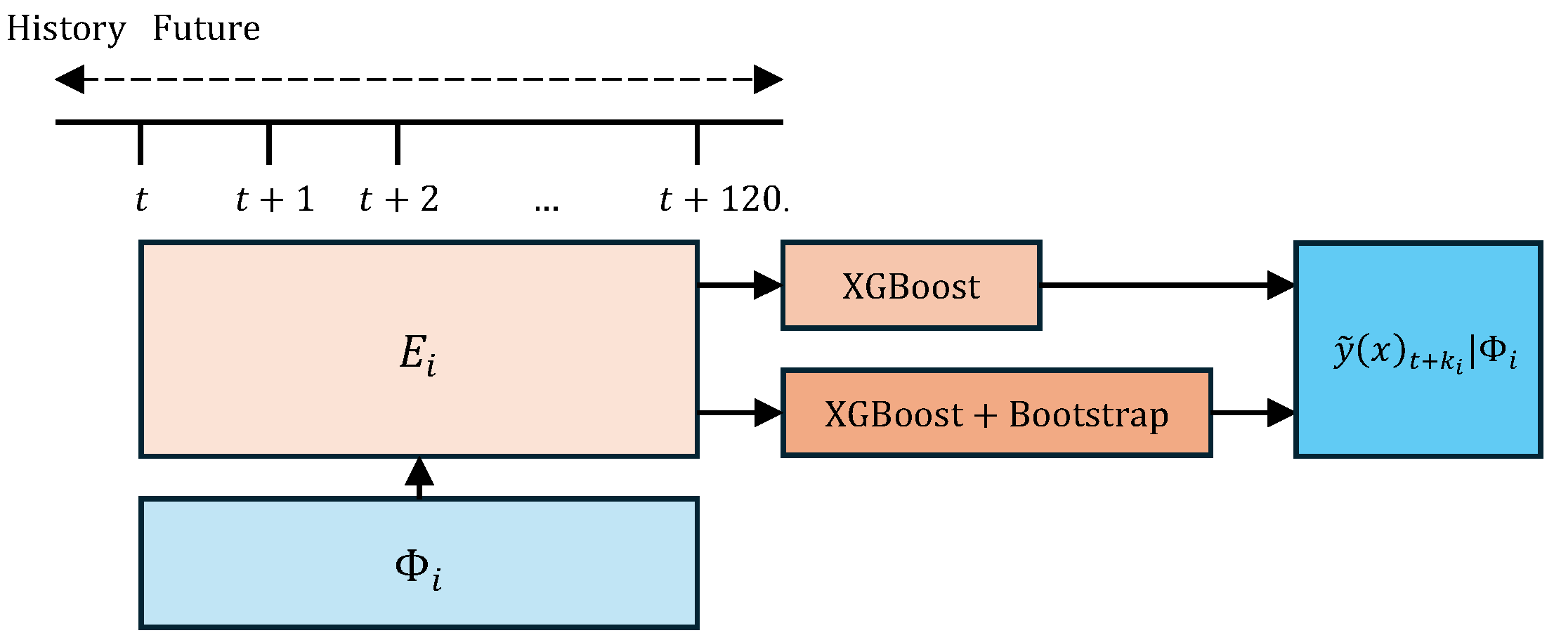
, where 61,225 is the number of input instances. This horizontally cascaded arrangement of the models is shown in
Figure 1; note that the forecasts are generated from the time of origin
t. Each model comprises a predictor, XGBoost or XGBoost + Bootstrap.
The selection of these specific horizons is motivated by their practical relevance in power system operations in Mexico. The 1-day-ahead forecast aligns with the regulatory framework established by CENACE [
3,
32], which requires next-day demand predictions for unit commitment decisions in the Day-Ahead Market (DAM). In contrast, the 5-day-ahead forecast supports broader operational planning and system security analyses, where extended forecasts are commonly used to anticipate system behavior under various scenarios [
19]. This dual-horizon approach ensures alignment with real-world decision-making practices in the Mexican electricity market.
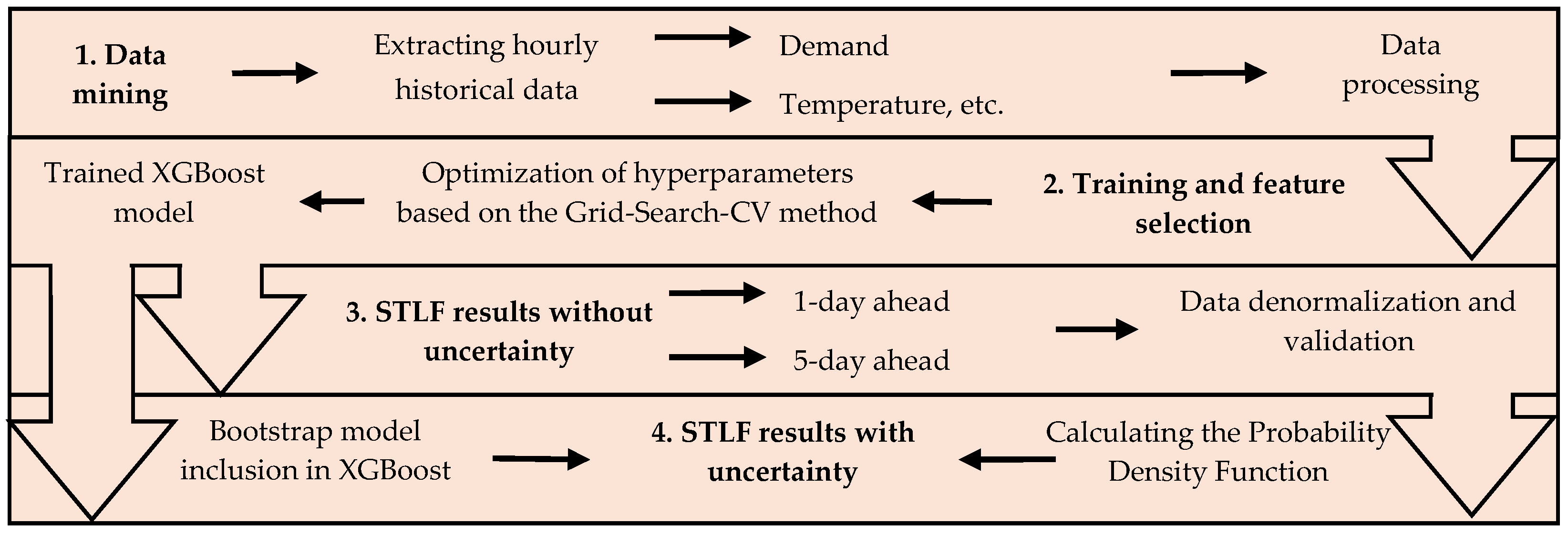
In the proposed methodology, the model’s inputs are updated automatically. This is achieved thanks to the interface design. In this way, the modeler can choose the area, the desired period, the inputs, and the model that best suits his needs. Considering its uncertainty based on the model XGBoost and Bootstrap, the STDF process is illustrated in
Figure 2, where it is observed that it consists of three phases, which are described below.
3.1. Data Mining
The record of the demand by area is available for consultation on [
30]. In data mining, the developed program uses the CENACE web service to obtain the data history of the demand for the selected zone for a consultation period and the desired control region established by the user. Due to missing or empty data, the file is first cleaned by removing any extra or blank rows. Then, missing dates are completed, and the dataset is prepared to impute missing, null, or negative demand values using the Autoregressive Integrated Moving Average (ARIMA) model. Since the historical demand data spans seven years and is initially expressed in MW, a Min–Max normalization is applied to scale all values within a standard range [0, 1]. This process ensures consistency across time steps and prevents variables with larger scales from dominating the forecasting model [
19].
3.2. Training of the Model
To begin model training, the dataset is split into input and test sets, with 80% of the data used for training and the remaining 20% reserved for testing. This division is performed using time series-specific techniques, which differ from traditional methods such as standard cross-validation by preserving the chronological order of the data. Rather than selecting data points randomly, the split ensures that the test set always follows the training set in time, thereby respecting the sequential nature of time series and preventing data leakage from future to past observations. This procedure ensures that the test sets are consistently positioned in the future relative to the training sets, thereby preserving the temporal integrity and chronological structure of the dataset. This is essential in time series since future data should not be used in the training stage, as it could lead to an optimistic evaluation of the model’s performance. Likewise, five “lags” or “temporal displacements” are defined to improve the performance of XGBoost or other regression methods as in [
2,
19], however, in this study, they are established as; t-120, t-720, t-1440, t-2160 and t-2880, which maintain the hourly granularity, since they are previous data that represent the demand values at that time, being used for training and improving the accuracy of the ML model [
19,
33].
Separately, to ensure the XGBoost model is optimally configured, a hyperparameter optimization is performed using Grid-Search with cross-validation. The ranges of values are shown in
Table 1 and establish the possible best hyperparameters, considering a combination of the ranges recommended in [
19,
28]. See
Section 2 for a detailed description of the hyperparameter optimization methodology.
3.3. Validation of the Forecast Results of the Models
Once the optimal hyperparameters for the XGBoost model have been determined, the forecasting period is selected, and the model is subsequently trained. The prediction process uses a maximum of 1000 iterations (n_estimators) and implements early stopping every 50 iterations (early_stopping_rounds) to halt training if no significant improvement is observed. Additionally, the initial prediction is based on the median of historical demand data (base_score). It is important to note that these hyperparameters are not optimized in this study, but rather fixed to predefined values, unlike the others previously tuned. After training, the data are denormalized for visualization, and both the predicted and actual demand values are plotted. The performance of the forecast is evaluated by calculating the following metrics: MAE, MSE, MAPE and RMSE, which are expressed in (
5), (
6), (
7) and (
8), respectively.
where
represents the actual observed demand value at time point
i,
represents the predicted demand value at the same time point generated by the model; and
n denotes the total number of data samples, i.e., the number of time points.
3.4. Considering Uncertainty in Forecasting: XGBoost and Bootstrap Methods
The forecast obtained from the previous steps is used to predict electricity demand while accounting for its associated uncertainty. To this end, the standard XGBoost model for regression is defined in Equation (
4). Let
denote the training dataset, where
represents the input features and
corresponds to the target variable, i.e., electricity demand in MW. The XGBoost model is trained by minimizing a regularized loss function that balances prediction accuracy and model complexity.
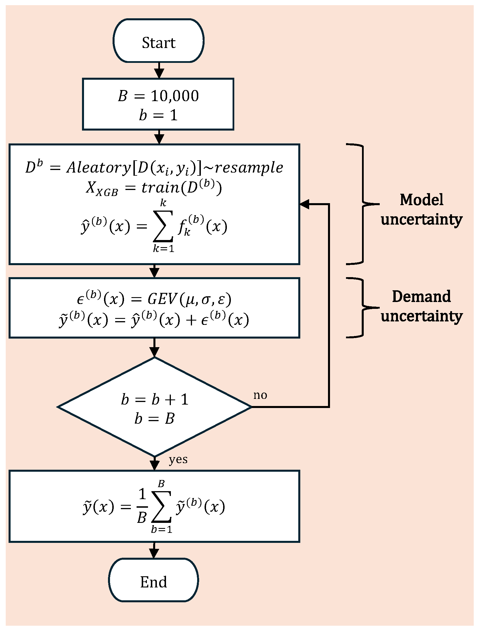
Once the forecasting model has been selected, its uncertainty is addressed using the Bootstrap method. Following the recommendation in [
22], we choose
B = 10,000 samples, as this number is sufficient to ensure stable estimates while keeping computational costs moderate. Let
, denote the resampled datasets, where each
is obtained by randomly resampling the training data
D with replacement. An XGBoost model is trained on each of these bootstrap samples:
where
is the
k-th tree trained in sample
. To model the uncertainty in electricity demand, a stochastic noise term
is added to each bootstrap prediction in (
9), having result as:
where
follows the probability density function of the electricity demand data, which is obtained by a goodness-of-fit test and corresponds to the generalized extreme value function; its parameters are calculated using the maximum likelihood estimated (MLE) method from the errors of the XGBoost model, then
,
,
and
, therefore, the final prediction
is the average of predictions with stochastic noise, as shown in (
11).
Then, the complete model can be expressed as:
The process above is exemplified in the diagram in
Figure 3.
The result is a forecast model where the uncertainty of the XGBoost is considered with the training of the resampling of the training data, with which obtains B different forecasts and due to the sample property of the model is added the uncertainty of demand in the form of stochastic noise adjusted to a function of probability density that represents the historical behavior of demand, so it is crucial to identify the density function of the study area to obtain a good forecast. Additional variables with stronger correlation can be included in the training set; However, it is essential to preserve the temporal relationships between these variables. Therefore, the Bootstrap resampling is applied by re-sampling only the rows of the training matrix D ensuring that the time-dependent structure within each observation is maintained.
The present study uses two models for STDF. The first is a base model based on XGBoost, while the second incorporates an improved approach using the Bootstrap technique to increase the robustness of the forecast.
Table 2 summarizes the main characteristics of each model.
4. Case Study
In Mexico, the CENACE forecasts electricity demand and prepares hourly projections per demand zone for both the day of operation and subsequent days. These forecasts are essential for the supplementary allocation of power plant units, ensuring the system’s reliability. During the trading day, the auto-regressive integrated moving average uses the most recent forecast to operate in the real-time market. The National Interconnected System (SIN), the Mexican electricity system, is divided into eight geographically distributed control areas. Each area [
32] has different behaviors due to variations in electricity consumption, illustrated in
Figure 4 that forecasts electricity demand and prepares hourly projections per demand zone for both the day of operation and the subsequent days.
The STDF will be carried out in the area called ZOTSE CFE, which covers the following demand zones: Tapachula, San Cristóbal, Tuxtla, Villahermosa, Chontalpa and Los Ríos, also shown in
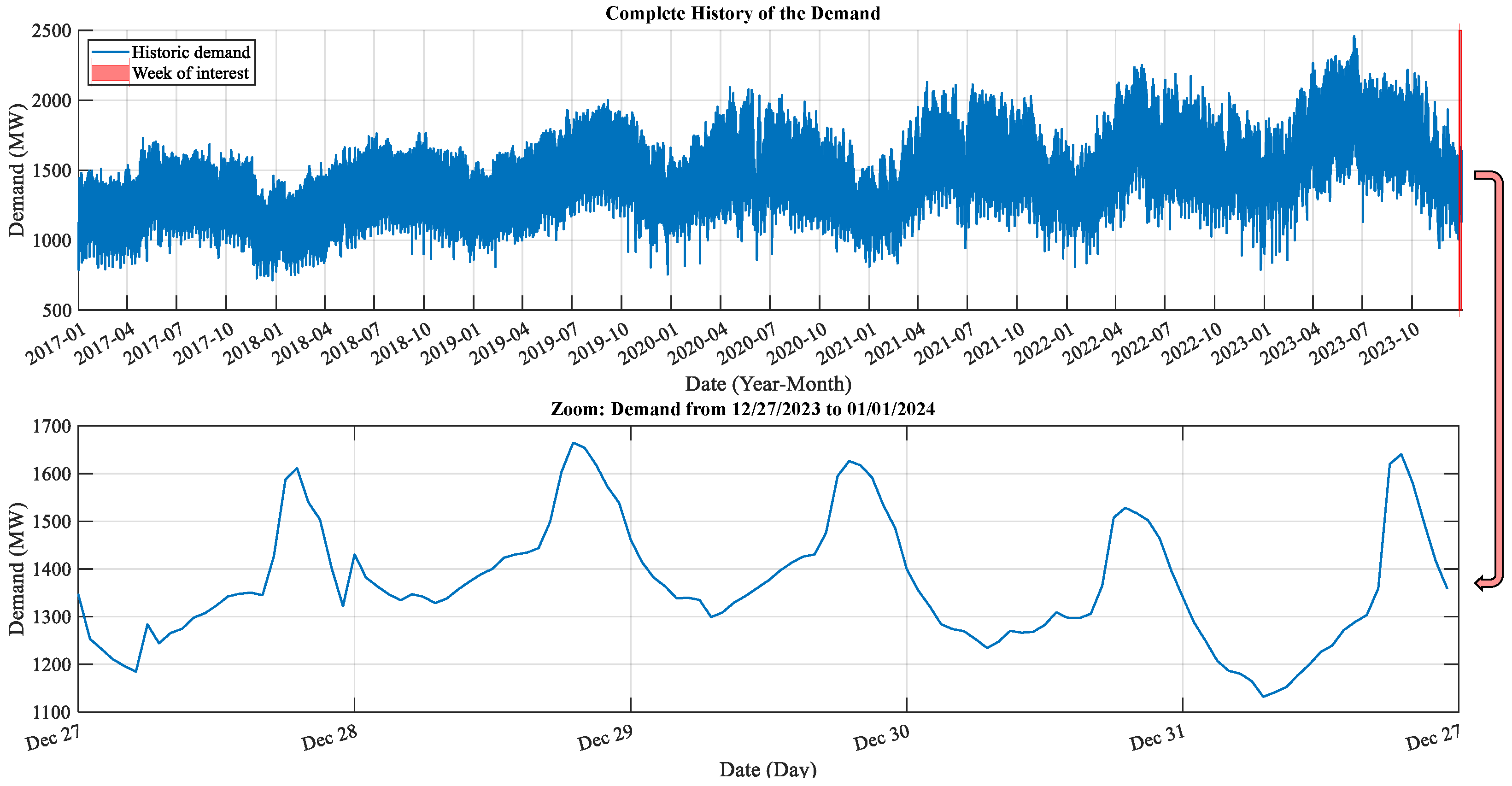
Figure 4; this is located in the Eastern zone which is the area of most significant participation in the SIN. Historical demand in this area is shown in
Figure 5. It should be noted that the choice of these nodes exemplifies the versatility of the forecasting tool, which can be performed in any node from the peninsular to Baja California Sur.
To confirm the effectiveness of the proposed method, experiments were carried out using the demand data set of the region in question, with the software and hardware configuration described in
Table 3.
5. Analysis of Results
The following is the analysis of the forecast results using the proposed model (XGBoost + Bootstrap) for 1-day and 5-days ahead. In two scenarios, stochastic noise is added to the forecast for the implementation of the proposed model since the density function used for the model results from the goodness-of-fit test made to the historical values of the demand, adjusted to the error of the Bootstrap method. It should be noted that 10,000 samples are considered for using the Bootstrap method with stochastic noise. The simulation has an average running time of 43 min. As expected, the computation time decreases proportionally when a smaller number of samples is used.
Simulations of different forecast times are carried out to compare the development of the model based on the metrics described in the previous section. Likewise,
Table 2 defines the scenarios to be simulated for both forecast times.
It should be noted that for all the scenarios described in
Table 2 the uncertainty of demand is considered in
and
, in addition to considering the temperature variable for the
and
, since, in the literature, an essential impact of the temperature uncertainty on the results of the forecast has been demonstrated [
11,
13,
20]. In our case study, the temperature used for model training corresponds to the average across the study areas. This approach is justified by the significant geographical separation between the areas, which could introduce outlier values that negatively affect forecast accuracy. By averaging the temperature, the model becomes more robust and less sensitive to local anomalies, thereby enhancing its overall performance.
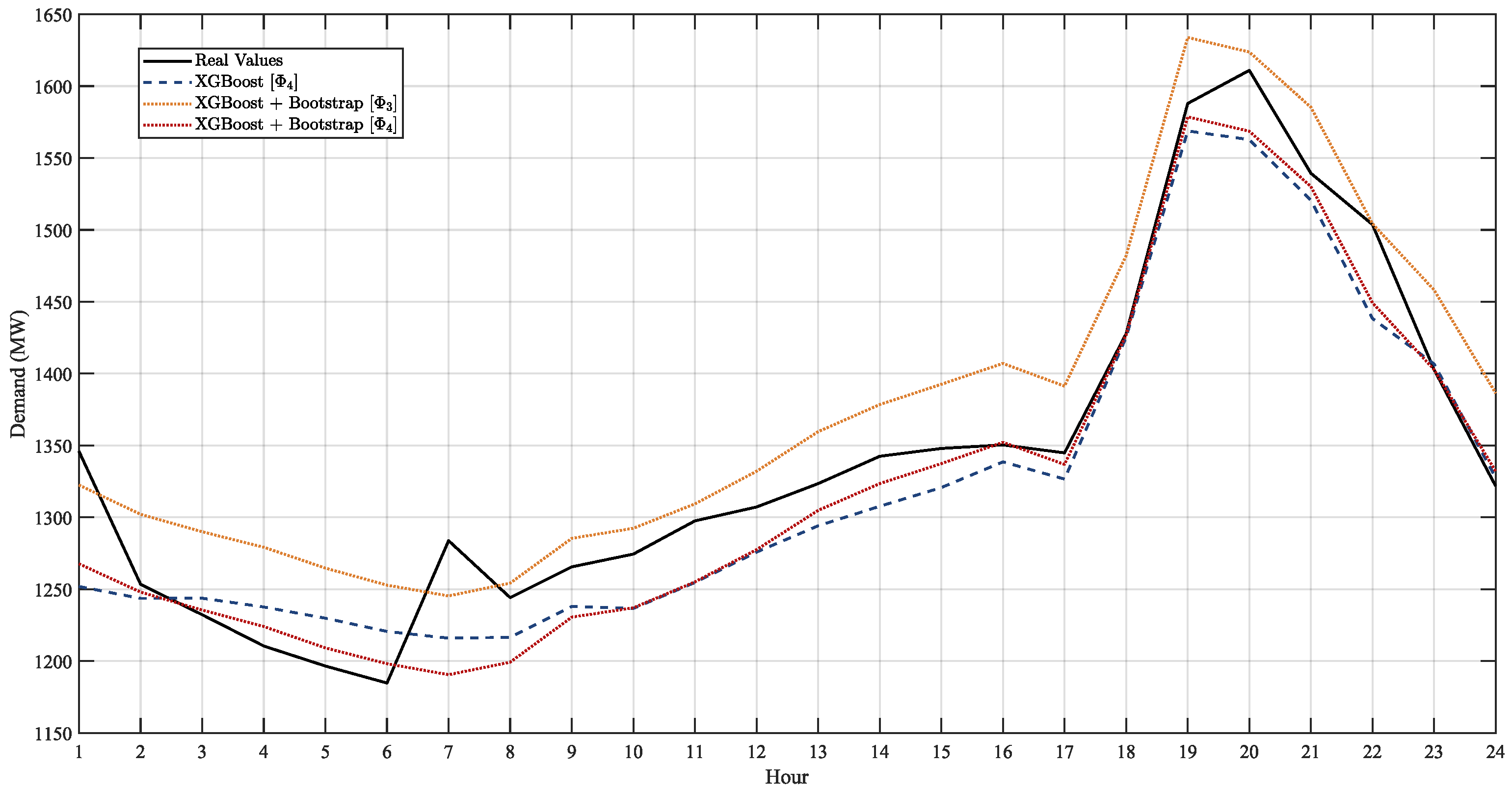
The following are the results for the 1 day forecast in advance in
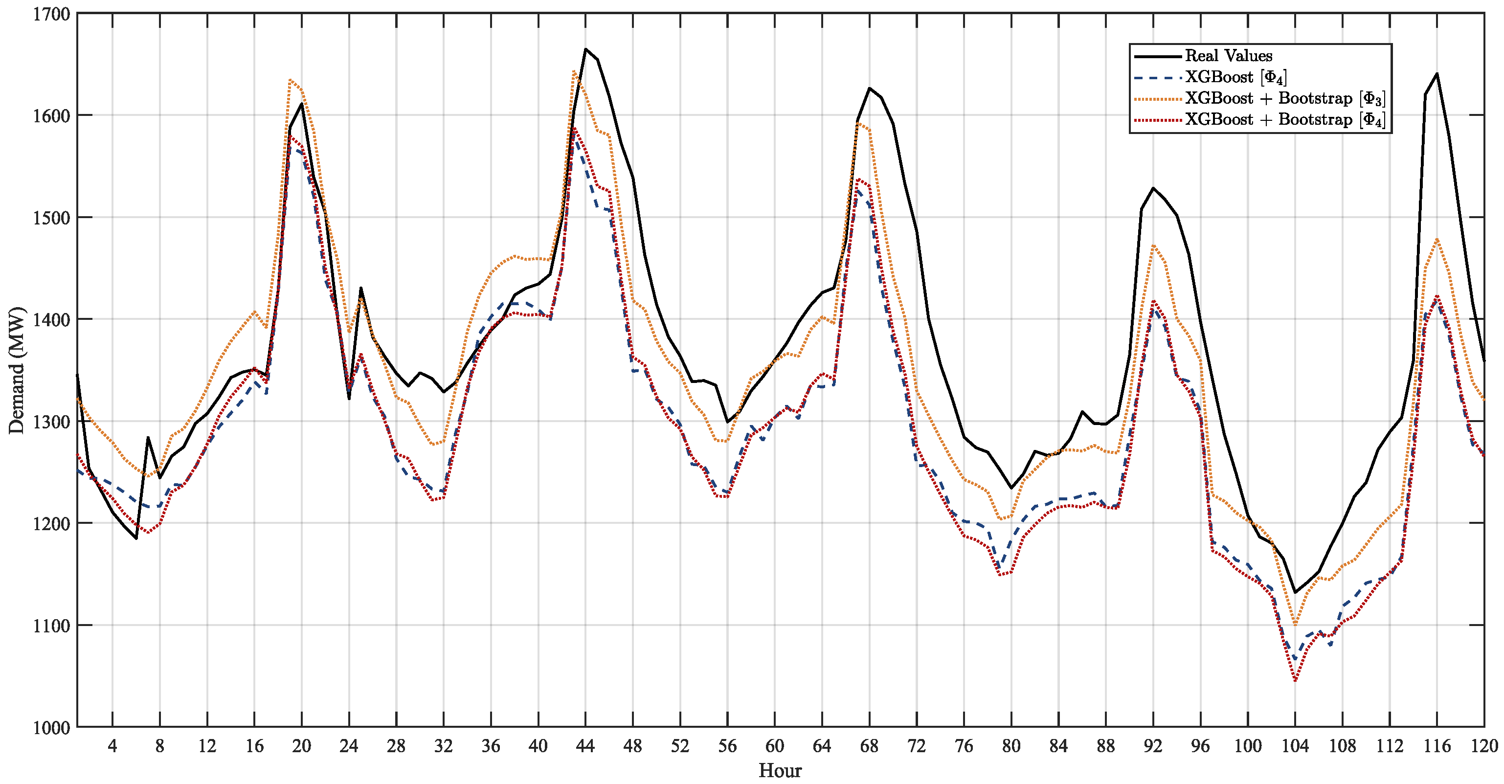
Figure 6 and the results for the 5-day forecast are found in
Figure 7.
To validate the results, the metrics mentioned earlier were calculated, comparing them with the actual demand values for the respective periods, 1-day ahead in
Table 4 and 5-days ahead in
Table 5.
5.1. Forecast Results Considering the Impact of Demand Uncertainty
Table 4 presents the one-day-ahead forecasting results for the XGBoost model and the proposed model, both with and without stochastic noise (
and
, respectively). The results indicate that the proposed model without stochastic noise achieves the best performance, with a MAPE of 2.200%, outperforming both the XGBoost model (2.331%) and the proposed model when stochastic noise is included (2.768% and 3.444%). These findings suggest that, for 1-day ahead forecasts, the inclusion of stochastic noise negatively impacts predictive accuracy. Therefore, the proposed model without stochastic noise is adequate for STDF. In
Figure 6, it can be observed that the forecast results obtained with the proposed model without stochastic noise are closer to the actual values. Similarly, the XGBoost model shows a reasonable approximation, although it is less accurate. In contrast, the proposed model with stochastic noise produces forecasts that deviate more significantly from the actual values, indicating that the inclusion of noise negatively impacts the model’s performance.
Likewise, in
Table 5 and
Figure 7, the results of the forecast are presented considering the uncertainty of demand for 5-day ahead of the Model XGBoost and the proposed model with and without stochastic noise. Contrary to the previous case, a better result of the forecast is observed when using the proposed model considering the stochastic noise obtaining a MAPE of 2.073%, in contrast to the XGBoost Model, which is 1.717 higher, as well as the proposed model without considering the stochastic noise shows deficient results with a MAPE of 4.358%. The above is because the more significant the forecast time, the greater the uncertainty to be considered, so considering stochastic noise within the model manages to mitigate the impact of the uncertainty of demand.
In
Figure 7, it is observed that the results of the forecast using the proposed model considering stochastic noise are close to the actual values. In this case, the poorest approximation is of the proposed model without considering stochastic noise since by not introducing this variable to the model, there is no additional tool to mitigate the uncertainty for an extended-term forecast.
5.2. Forecast Results Considering the Impact of Temperature Uncertainty
Table 4 presents the forecasting results for one day ahead, considering demand and temperature uncertainty, for both the XGBoost model and the proposed model with and without stochastic noise (
and
, respectively). Once again, the proposed model without stochastic noise (
) demonstrates the best performance, achieving a MAPE of 1.644%, which confirms its effectiveness for short-term forecasts and its ability to handle different sources of uncertainty. The XGBoost model also yields a good result, with a MAPE of 1.778%. In contrast, the inclusion of stochastic noise in the proposed model (
) negatively affects its performance, as evidenced by the higher MAPE of 3.444%. In
Figure 6, it can be observed that the forecast results, when considering temperature uncertainty, are more accurately approximated to the actual values when using the proposed model without stochastic noise, as well as the XGBoost model. In contrast, the proposed model with stochastic noise shows less precision, consistently overestimating the actual values.
In
Table 5, the results of the forecast are shown considering the uncertainty of the demand and temperature for 5-day ahead of the XGBoost Model y of the proposed model with and without stochastic noise. Where the impact of the temperature uncertainty is reflected when obtaining higher error metrics compared to the previous section. Likewise, the mitigation of uncertainty is observed when considering the stochastic noise, since when implementing the proposed model with stochastic noise, it obtains a MAPE of 2.073%, considerably lower compared to the Model XGBoost (4.846%), and the proposed model without stochastic noise (5.123%).
In
Figure 7, it is observed that the forecast results, when considering the uncertainty of the temperature, are better with the proposed model and stochastic noise since they are more accurately approximated to the actual values. For this case, the XGBoost Model and the proposed model, without stochastic noise, are significantly far from the actual values. So again, the impact is reflected in the forecast, involving a source of additional uncertainty, such as the case of temperature.
6. Conclusions
This paper focused on electricity demand forecasting, considering its uncertainty by combining a stochastic approach with novel prediction methods so the proposed methodology can be adapted to different machine learning methods and large scales of electricity demand. Also, considering different sources of uncertainty in the variables of electrical energy consumption and temperature, with the Bootstrap method and stochastic noise, the result is a hybrid machine learning and probabilistic model. The uncertainty model with the Bootstrap method considers random samples in the XGBoost training and consequently for the prediction, where each one represents a probability, then calculating the average, we can get a punctual forecast, however as can be seen in the metrics obtained, only with the Bootstrap method a MAPE of 4.358% is presented when the 5-day ahead forecast is made only with electricity demand data, so by including the temperature variable a MAPE of 5.123%, is obtained, therefore it is concluded that using this model for forecasting of more than 24 h is not adequate, since the uncertainty is more significant and produces larger errors as the time to predict increases. On the other hand, the case of the 1-day ahead forecast offers better results with a MAPE of 1.644%, integrating the temperature into the training set. The complete model strongly correlates with its density function since the term stochastic noise of the demand in the bootstrap method is considered. Better results are obtained in the case of five days with a MAPE of 3.042% considering the temperature and 2.073% without this variable. Still, for the case of 1-day ahead, the stochastic noise provides a more significant source of error; in this way, the model without this term is sufficient if more variables are considered for training, such as the temperature of the area of study, so it is appropriate to conclude that the model can be adapted both for the short term (1 day) and the extended- term (5 days) in areas of high demand and with electrical variability such as the area of southeastern Mexico.


 ,
, 

