A Set of New Tools to Measure the Effective Value of Probabilistic Forecasts of Continuous Variables

Abstract

In recent years, the prominence of probabilistic forecasting has risen among numerous research fields (finance, meteorology, banking, etc.). Best practices on using such forecasts are, however, neither well explained nor well understood. The question of the benefits derived from these forecasts is of primary interest, especially for the industrial sector. A sound methodology already exists to evaluate the value of probabilistic forecasts of binary events. In this paper, we introduce a comprehensive methodology for assessing the value of probabilistic forecasts of continuous variables, which is valid for a specific class of problems where the cost functions are piecewise linear. The proposed methodology is based on a set of visual diagnostic tools. In particular, we propose a new diagram called EVC (“Effective economic Value of a forecast of Continuous variable”) which provides the effective value of a forecast. Using simple case studies, we show that the value of probabilistic forecasts of continuous variables is strongly dependent on a key variable that we call the risk ratio. It leads to a quantitative metric of a value called the OEV (“Overall Effective Value”). The preliminary results suggest that typical OEVs demonstrate the benefits of probabilistic forecasting over a deterministic approach.

1. Introduction

Probabilistic forecasts have become an important topic in several scientific fields, like meteorology, finance, decision science and management science. They are produced in order to improve decision-making [1]. Historically, the literature has shown that the costs of weather-dependent activities operated with the help of deterministic forecasts are not necessarily related to these forecasts’ accuracy [2], highlighting the benefits of using probabilistic weather forecasting. Over recent years, work on probabilistic forecasting has spread into several research fields, including macroeconomy [3,4,5], sport [6], finance [7,8,9,10] and meteorology [11,12,13,14,15].

In parallel with these developments, the research community has proposed several methods to evaluate the quality of probabilistic forecasts [16,17], which is defined as the correspondence between forecasts and corresponding observations [18]. The need for proper scores to assess quality is now widely acknowledged. As numerous such scores exist, the debate over their desired properties and comparative advantages remains active. However, these procedures do not provide insight into the operational benefits, also referred to as the value (or utility) [18], of probabilistic forecasts. This represents a major limitation, since the achievement of a sufficient value gain is the only way to justify efforts to study and generate probabilistic forecasts.

Assessing this value is complex because it requires the integration of forecasts into the decision-making process. This is the primary objective of this work. The value of forecasts depends on how they are used, and must be evaluated in terms of the benefits derived from decisions based on these forecasts [19]. Accordingly, a framework that simulates forecast use and quantifies the losses associated with errors is required. It should reflect actual operational or industrial costs, and may not necessarily be subject to the constraints of quality assessment frameworks (properness, locality, etc.).

Either categorical events or continuous variables can be subject to forecasts. On the one hand, categorical events can only belong to a finite number of categories (e.g., whether it rains or not). Practical applications can involve numerous categories [20], but usually, and for simplicity, most focus on binary events. On the other hand, continuous variables can take any value from an infinite set of admissible values (e.g., the amount of rainfall). In this case, the probabilistic prediction can be given equivalently by its probability density function (“PDF”) or its cumulative distribution function (“CDF”) [21].

The value of probabilistic forecasts has been mostly studied for binary events. The integration of these forecasts into decision-making is typically modeled using the cost–loss framework [22,23]. Thereby, the concept of the “utility” of probabilistic forecasts of binary events has been introduced. Since the work of Murphy [24,25], this utility has been more frequently called “value”, especially in meteorology. The cost–loss situation has become a generic methodology for the assessment of the potential value of such binary probabilistic forecasts [23,24,26,27,28]. This assessment is based on the reduction in losses achieved by using a specific forecast [19,29]. It should be noted that a comparison of probabilistic and deterministic forecasting has been carried out using this methodology [30].

This procedure is nonetheless only valid for categorical events, while the value of probabilistic forecasting of continuous variables has been barely studied [31,32]. Given the central role of the cost–loss framework in evaluating categorical forecasts, this study aims to lay the groundwork for extending such a methodology to continuous forecasts. A unified framework would also facilitate fairer comparisons of results across applications. In this work, we propose a framework based on several visual tools and one quantitative metric to evaluate the value of probabilistic forecasts of continuous variables for use in various applications. In this study, we propose a methodology that is only valid for the specific class of piecewise linear cost functions. This is a major limitation, as real-world cost functions can be more complex. However, the proposed methodology is intended not to be universally applicable, but rather to serve as a first step towards a general and adaptable evaluation framework. Moreover, previous studies have shown that such cost structures do arise in practice, shedding light on these cost functions [33].

The structure of this paper is as follows. Section 2 recalls some methodological tools used to study the value of probabilistic forecasting of binary events. Section 3 introduces a mathematical model of the costs associated with the usage of probabilistic forecasts of continuous variables, and presents the fundamental hypothesis of our methodology. Section 4 details the proposed methodology and its implementation. The crucial role of risk distribution is highlighted in Section 5. Section 6 shows an application of the proposed methodology to a simple case study. Finally, our conclusions are presented in Section 7.

2. The Value of Probabilistic Forecasts of Binary Events

In this section, we would like to recall the generic and sound methodology which is widely used for the evaluation of the value of probabilistic forecasts of binary events. It provides a basis for the new methodology for the assessment of the value of probabilistic forecasts of continuous variables that is proposed in Section 4.

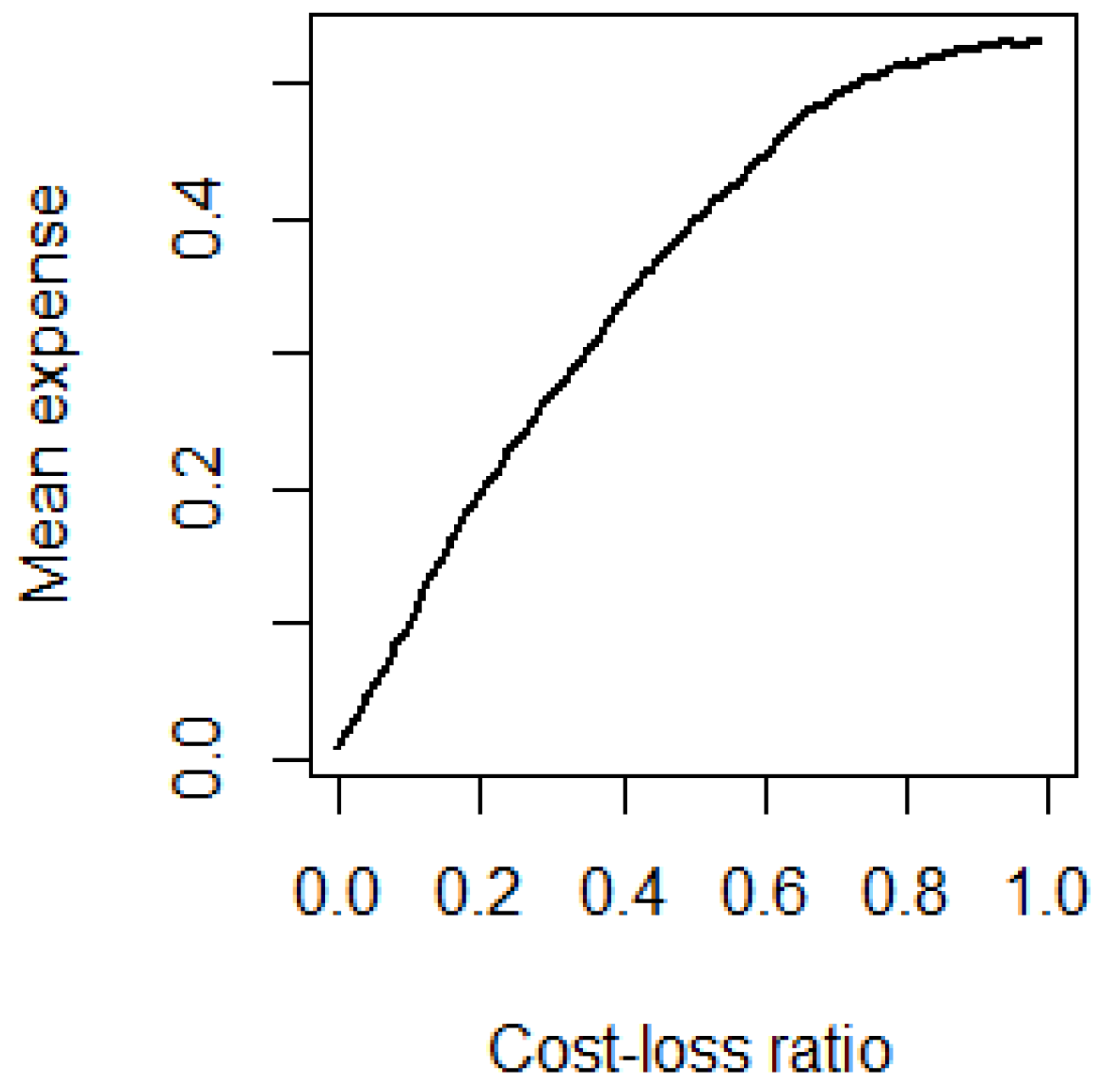
2.1. The Cost–Loss Situation

Let us consider the following situation: a binary event can either materialize or not. A probabilistic forecast gives prior information to a decision-maker about the probability of this event, which generates a loss L. However, the decision-maker can protect against this risk at a cost C. This situation is known as the cost–loss situation [24]. Usually, the possible outcomes and expenses E faced by the user are outlined by a contingency table, as represented in

Table 1. A contingency table of the possible outcomes and associated expenses in a cost–loss situation.

		Outcome
		Yes	No
Protection	Yes	Hit	False alarm
		C	C
	No	Miss	Correct rejection
		L	0

[19].

For fixed values of C and L, the mean expense $E_m$, which can be expressed in “arbitrary monetary units” [30], is calculated as follows:

$$E_m=(a+b)\times C+c\times L,$$

(1)

where a, b and c are, respectively, the relative frequencies of hits, false alarms and misses.

In the cost–loss situation, [23] shows that the optimal decision is to protect against the risk (pay C) as soon as the forecast probability of occurrence exceeds the cost–loss ratio $C/L$. Once this optimal rule has been followed, the mean expense $E_m$ becomes a key metric for evaluating the value of a specific forecast. The value of a forecast $\widehat{F}$ depends on the cost–loss ratio $C/L$, and plotting $E_m$ as a function of the cost–loss ratio (the “cost diagram”) is a recommended practice [34], as illustrated in Figure 1.

2.2. Benchmarking with Climatology

A cost diagram is an appropriate tool for estimating the total costs associated with decisions based on a probabilistic forecast. However, the choice of a probabilistic forecast should rather be justified by the benefits gained from its usage. Indeed, according to Richardson in [29], a forecast has value if “the user decides on actions he would not otherwise take”. This implies the existence of another benchmark decision model that is used to take actions by default. The value is then defined by the relative difference in terms of costs between the two models [35]. The common practice is to consider the empirical distribution of past observations as a benchmark naive forecasting model. This simple model, called a climatological forecast in the meteorology community, is generally preferred, since it is both probabilistic and very easy to build. In addition, it requires no information about the future, since it is based only on past data [36] (although climatology is the most common benchmark model, others can be considered as well [37]).

In order to compare the expenses induced by a particular forecast $\widehat{F}$ and the climatology forecast, it is a good practice to consider the relative economic value (“REV”), defined as

$$REV={\displaystyle \frac{E_{CLIM}-E_{\widehat{F}}}{E_{CLIM}-E_p}},$$

(2)

where $E_{CLIM}$, $E_p$ and $E_{\widehat{F}}$ are the expenses associated, respectively, with the climatology, a perfect forecasting model (i.e., forecasts always equal to observations) and the evaluated forecast.

The potential economic value ($PEV$) of a binary forecast is the entire set of its relative economic values for all $C/L$ ratios between 0 and 1. The $PEV$ is usually displayed as a plot of the $REV$ against the $C/L$ ratio, which fully qualifies a forecast and quantifies its merits versus the “no-skill” climatology forecast. In [28], the author studied the $PEV$ of ECMWF forecasts for the probability that 24 h precipitation would exceed 5 mm, a threshold linked to flood events. The results are shown in Figure 2. Note that the $REV$ is simply called “VALUE”. A notable difference in favor of probabilistic forecasts (“EPS”) is found. The control forecast is beneficial compared to climatology for small ranges of cost–loss ratios, but never saves more than 25% of the losses. In contrasts, the EPS forecast is more efficient and saves up to 50% of the losses compared to climatology (for a cost–loss ratio of 0.1).

Many other examples of the use of this methodology to gauge the value of binary forecasts across various applications can be found in the literature [27,38]. Wilks [27] links it to the well-known ROCs (“Relative Operating Characteristics”), discusses cases where a model underperforms in climatology, and, more importantly, demonstrates how a user can adapt this metric to the cost–loss ratios relevant to their decision problem. The cost–loss ratio axis is reduced to the relative frequency of faced costs, and the plot collapses into one single number. This methodology is straightforward, easy to understand and widely applicable. This is why its extension towards the probabilistic forecasting of continuous variables is the focus of this work.

3. The Value of Probabilistic Forecasts of Continuous Variables: Theory and Hypothesis

In order to propose a methodology for the evaluation of the value of forecasts of continuous variables, it is first necessary to establish some assumptions. To this end, we emphasize, in this section, the importance of the user’s cost structure, and highlight some key properties that emerge from it.

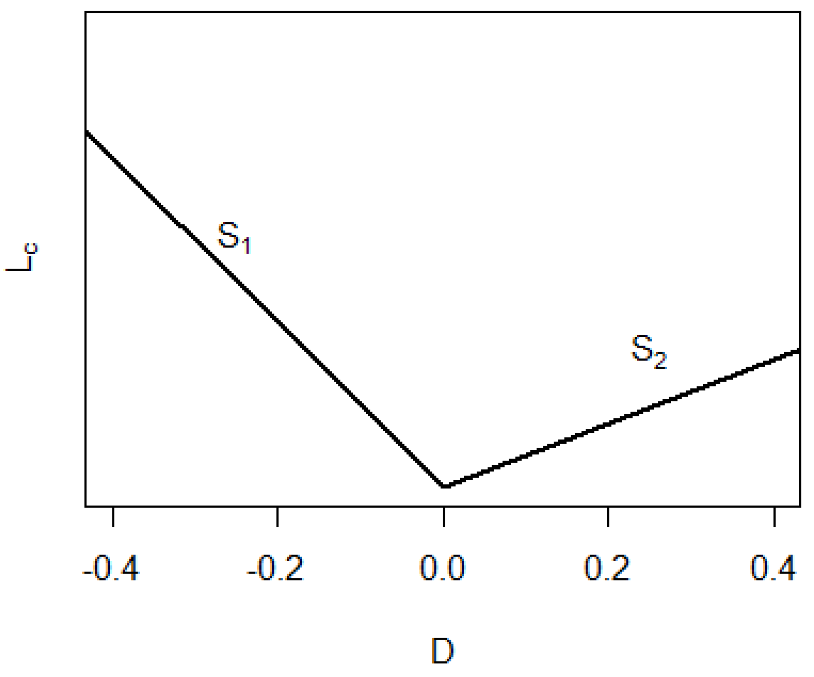
3.1. The Underlying Decision-Making Process and the Importance of Cost Modeling

The value of a forecast refers intrinsically to the user side and to the benefits gained from employing a particular forecast. Understanding the decision-making process of the user is therefore a necessity for assessing forecast value. In general, this decision-making process implies, to some extent, losses for the user, and the forecast is used to minimize them. Note that the losses are not necessarily financial, but could also be environmental, technical or other types of losses. They are, in general, a combination of losses of different natures.

In this study, we only consider decisions which are deterministic and algebraic, which is a very common case, for instance, when a forecast is used for sizing an energy volume [39] or some physical flow [33].

Thus, the difference D (also called the deviation) between the actual outcome Y and the decision taken T can be calculated as

$$D=Y-T.$$

(3)

The resulting loss (noted here $L_c$, as it is associated with continuous variables) should be modeled as a function depending on the deviation D. Such a function is called a loss function [40]. A simple and widely applicable loss function has been identified by [41], and is called the “market-based loss function” by [42].

A market-based loss function is a piecewise linear function characterized by a negative slope of absolute value, $S_1$, for $D<0$, and a positive slope $S_2$ for $D>0$. The minimum loss is zero, and is reached for $D=0$. An example of such a function is represented in Figure 3. Note that we make the strong assumption that the loss function is fully known in advance by the forecaster. In real-world situations, it might not be true, requiring forecasters to also predict $S_1$ and $S_2$. Although forecasting cost slopes is beyond the scope of this study, it may be crucial in practice. Forecast errors can lead to suboptimal decisions and may lead to additional costs.

The restriction to piecewise linear loss functions is primarily motivated by the relative prevalence of these costs in real-world decision problems. However, other types of costs may also be of interest. For instance, logarithmic costs are thoroughly discussed in the quality assessment evaluation framework, yet they seem to be encountered less frequently in practice. For market-based loss functions, ref. [41] highlights a crucial property: the optimal decision $T_o$ (i.e., the one that minimizes the expected loss) is always

$$T_o={\widehat{\mathcal{F}}}^{-1}\left({\displaystyle \frac{S_2}{S_1+S_2}}\right),$$

(4)

where $\widehat{\mathcal{F}}$ is the forecast CDF of the variable of interest (e.g., energy volume, etc.). This result highlights the importance of the slope ratio $R={\displaystyle \frac{S_2}{S_1+S_2}}\in [0,1]$ (more simply called the “R ratio” hereafter). A ratio outside $[0,1]$ indicates that gains are generated when the decision deviates from the outcome, which seems highly implausible in real-world situations. $R=0$ reveals that a deviation of $D>0$ has no impact on the decision-maker. When $R=1$, the loss is null for a negative deviation. Put differently, given a forecast CDF $\widehat{\mathcal{F}}$, the optimal decision is defined by the quantile forecast of the level of probability $\tau =R$. In various cases where the forecast is not a full CDF (a common case is an ensemble forecast), deriving the optimal decision from the original forecast might include some numerical approximations.

With these notations, the effective loss becomes

$$L_c=\left\{\begin{array}{cc}(S_1+S_2)\times R\times D\hfill & \mathrm{if}D\ge 0,\hfill \\ (S_1+S_2)\times (R-1)\times D\hfill & \mathrm{if}D<0.\hfill \end{array}\right.$$

(5)

Equation (5) naturally highlights the sum $\gamma =(S_1+S_2)$ in the calculation of the effective loss. $\gamma$ outlines the potential cost of a decision, which can be interpreted as the level of risk.

Therefore, when the losses can be modeled by market-based loss functions, the decision-making context can be fully described by two fundamental indicators: R and $\gamma$. Whereas R accounts for the dissymmetry of the risk of a decision, $\gamma$ characterizes the level of risk associated with a single decision.

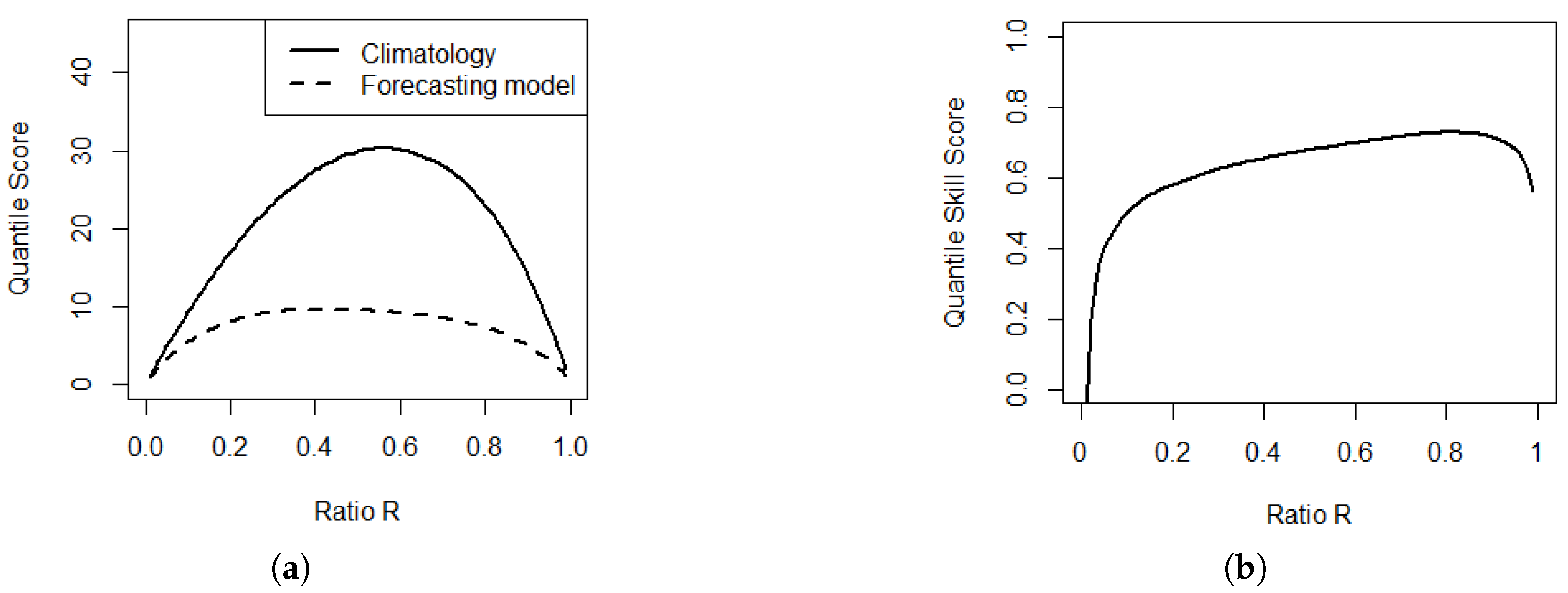
3.2. The Link with the Quantile Score

The quantile score ($QS$) is a widely used metric tailored to evaluate the quality of a forecast for a specific quantile $\tau$ (or “level of probability”). This numerical score has been recommended by [43] for the verification of solar irradiance probabilistic forecasts, notably because it is a proper score. Other scoring rules with different desirable properties are also commonly used, such as the logarithmic score (locality) [44] or the quadratic score (symmetry) [45]. QS calculation is based on the asymmetrical “pinball loss function” ($\rho$), defined as

$${\rho }_{\tau }({\widehat{F}}_{\tau },Y)=\left\{\begin{array}{cc}(Y-{\widehat{F}}_{\tau })\times \tau \hfill & \mathrm{if}Y-{\widehat{F}}_{\tau }\ge 0,\hfill \\ (Y-{\widehat{F}}_{\tau })\times (\tau -1)\hfill & \mathrm{if}Y-{\widehat{F}}_{\tau }<0,\hfill \end{array}\right.,$$

(6)

where Y is the outcome and ${\widehat{F}}_{\tau }$ is the forecast corresponding to a quantile with the nominal proportion $\tau$, i.e., ${\widehat{F}}_{\tau }={\widehat{\mathcal{F}}}^{-1}\left(\tau \right)$.

The QS can simply be calculated as the mean of the pinball functions for a set of forecast/observation pairs. It is positive and denotes a deviation from the perfect forecast (the lower the better). For a more exhaustive presentation of the QS, the reader is referred to [46,47].

It is worth noting that the effective loss experienced by a user facing market-based loss functions (see Equation (5)) is exactly equal to the pinball loss function (after identifying T to ${\widehat{F}}_{\tau }$), multiplied by $\gamma$. This provides a clear connection between the quality and value of forecasts. Therefore, this link can be used advantageously. Indeed, since the quality of probabilistic forecasts has been extensively studied, and since sound frameworks have been proposed by the scientific community, this comprehensive effort provides benefits for quality evaluation to assess the value of forecasts.

4. A New Diagnostic Tool to Assess the Value of Forecasts of Continuous Variables in Real Cases: The EVC

The purpose of this section is to take advantage of the notable properties established in Section 3 in order to propose a sound methodology to evaluate the value of probabilistic forecasts of continuous variables. In Section 4.1, we introduce the notion of potential value and demonstrate that the quantile skill score diagram is a suitable quality-based proxy for assessing it. Then, in Section 4.3, we propose a new tool called the EVC to assess the effective value of a forecast, taking into account the user’s cost structure, through a tool called the risk distribution diagram. We also introduce a related scalar metric, the OEV (Overall Effective Value).

The proposed framework is considered to be conceptually and practically aligned with the proven methodology for the study of the value of forecasts of binary variables reviewed in Section 2. This new framework can thus be interpreted as an extension of the latter to cases involving continuous variables.

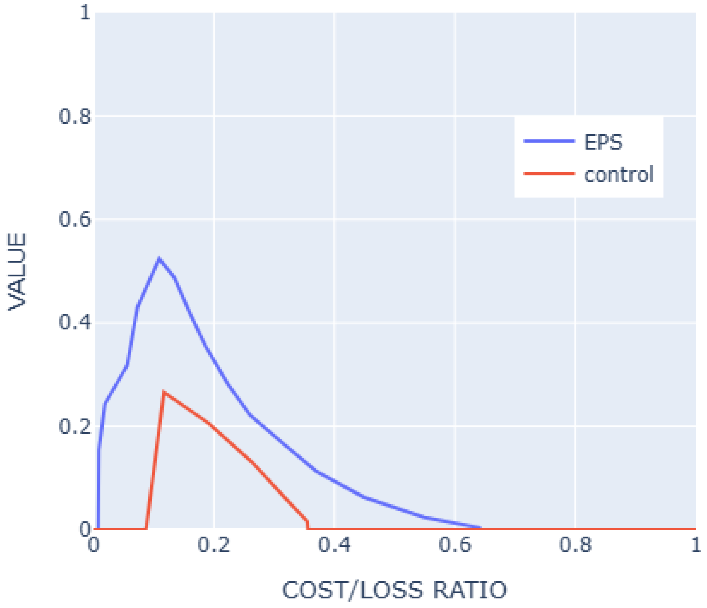
4.1. The Potential Economic Value of Forecasts of Continuous Variables

Similarly to previous works (see Section 2) that have used the potential economic value as a relevant indicator to assess the potential value of a binary event forecast, here, we propose a method to analyze the potential value of a probabilistic forecast of a continuous variable.

As demonstrated previously, the quality of a forecast for a fixed level of probability fully determines its value. Consequently, we first compute the quantile score (QS) of the forecast as a function of the level of probability (ranging from 0 to 1).

A quantile score diagram is a plot of the quantile score of a forecast against the probability level $\tau$. Note that this tool was originally constructed for the assessment of the quality of probabilistic forecasts [43], and has also been called the “Quantile decomposition of the CRPS” [48] in the literature. Its use can be extended to assess the value of a forecast, and should stand for the potential economic value of a probabilistic forecast of a continuous variable. Specifically, it indicates the potential losses associated with the use of a particular forecast, for all possible values of the R ratio.

Furthermore, replicating the good practices associated with the methodology for the assessment of binary event forecasts [29], we believe that the value should be judged in comparison with the climatology forecast, since the latter can be solely and easily performed based on minimal knowledge: the historical data at hand. Thus, we promote the use of quantile skill score diagrams. The quantile skill score (QSS) is defined as follows (knowing that the quantile score of a perfect forecast is null):

$$QSS=1-{\displaystyle \frac{Q{S}_{\widehat{F}}}{Q{S}_{CLIM}}},$$

(7)

where $Q{S}_{CLIM}$ is the quantile score of the climatology. It varies from 0 (no-skill forecast) to 1 (perfect forecast). A plot of the QSS across all values of $\tau$ is called a quantile skill score diagram in the quality assessment framework. We show that it also quantifies the level of the user’s loss reduction compared to the climatology for each ratio. Thus, using the skill score is a good proxy to assess the value, whereas it might be irrelevant for quality assessment (a skill score is, in general, not suitable). As this measure is still irrespective of the user’s cost structure, it provides information about the potential value of this forecast, and we claim that it could be also called the PEVC (“Potential Economic Value of forecast of Continuous variable”) in more value-oriented terminology. The effective value is obtained when the user’s specific loss functions are taken into account.

Figure 4 shows an example set of a quantile score diagram and a quantile skill score diagram for a forecasting model. The ratio axis has been discretized into 100 equally spaced bins. Note that a coarser resolution may introduce interpretation biases.

Contrary to the quantile score diagram, which is negatively oriented, a good forecasting model should exhibit high quantile skill scores, as close as possible to 1, for all ratios R.

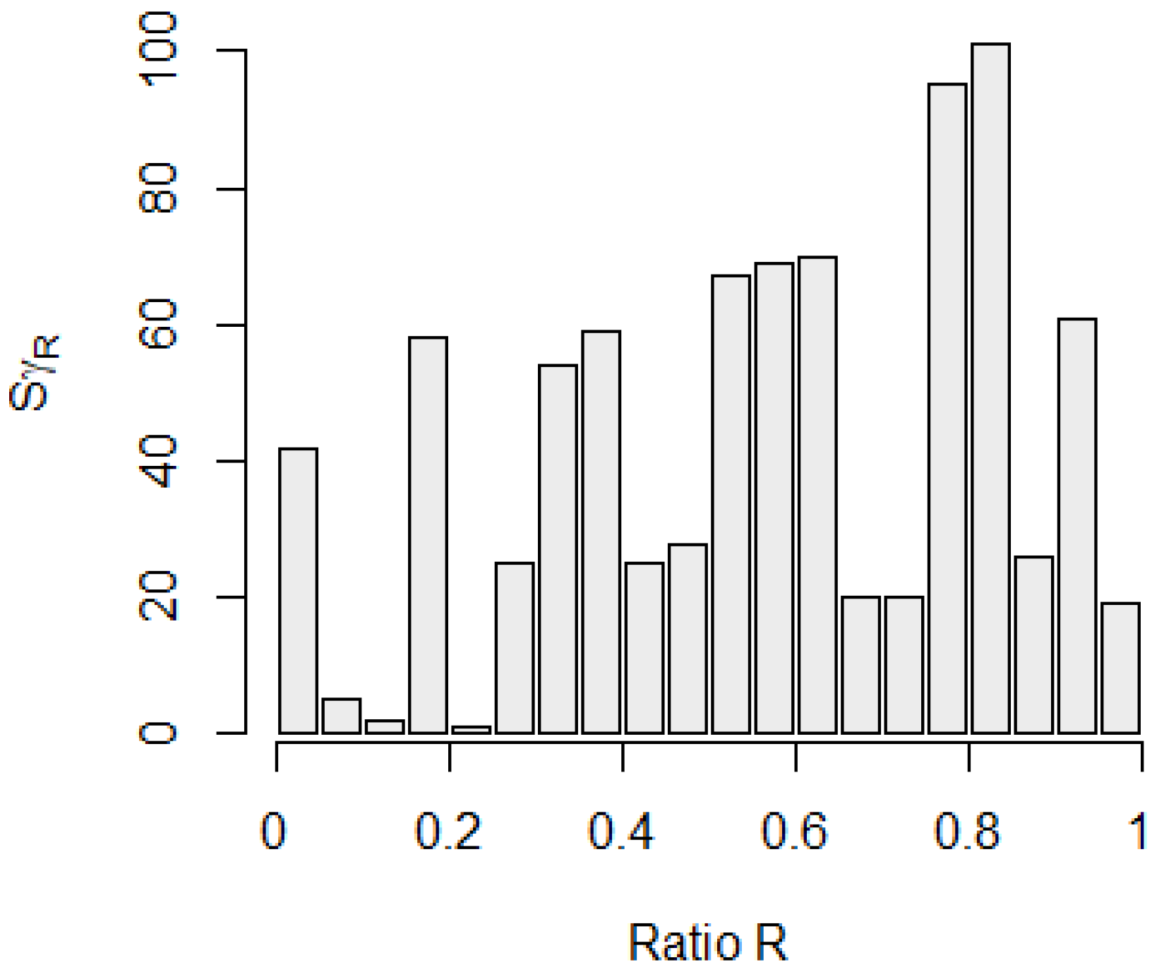
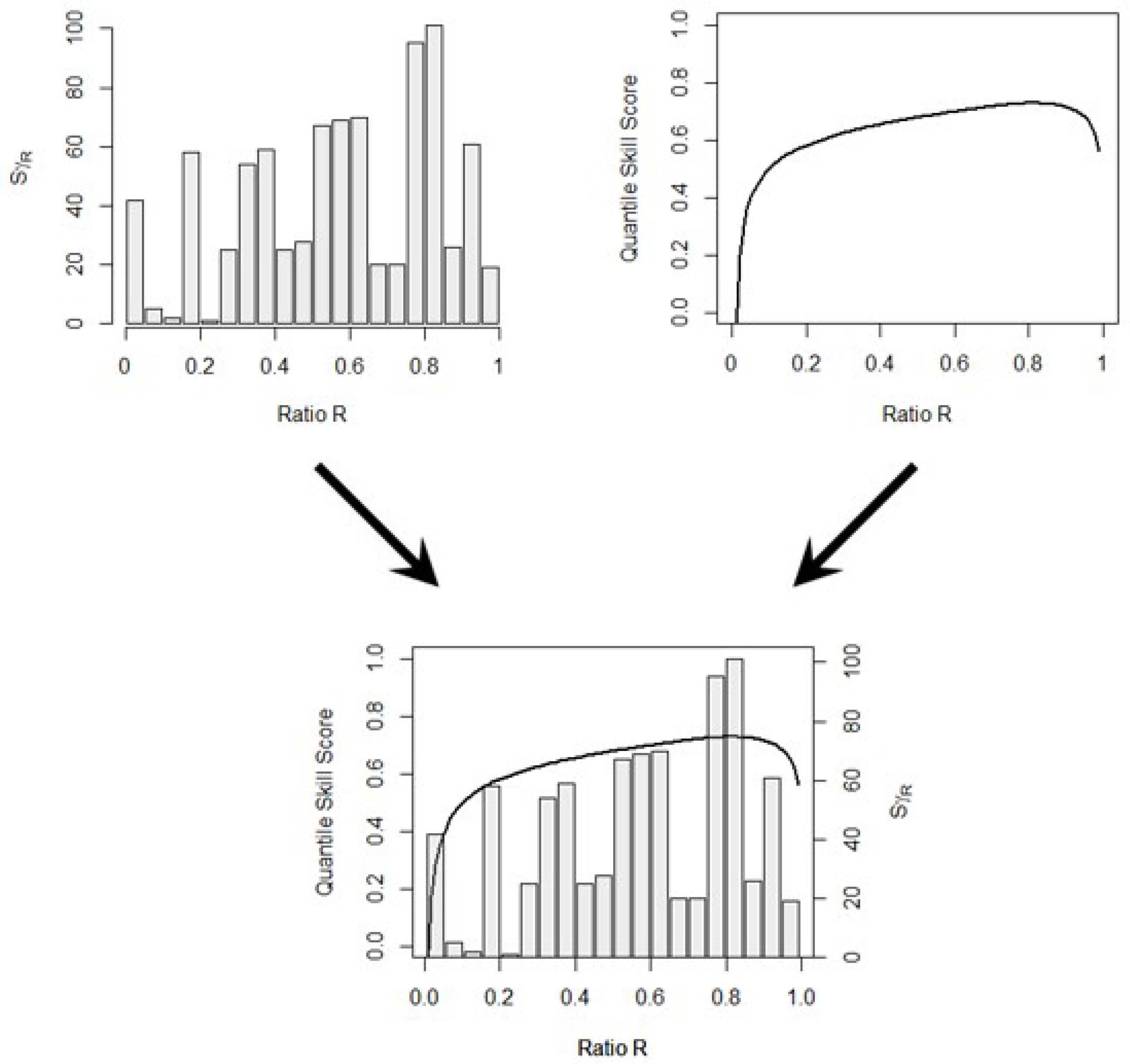
4.2. The Risk Distribution Diagram

Under market-based loss functions, the optimal decision that a decision-maker should take can be found analytically, and depends only on the two indicators $\gamma$ and R (see Equation (4)). However, decision-makers are commonly faced with sets of decision-making problems where these parameters can vary. In this case, it is preferable to evaluate the set of forecasts rather than the individual forecasts.

Considering that the pair $\{R,\gamma \}$ entirely summarizes the cost structure, it seems natural to represent a practical case in a diagram, which we will call the “risk distribution diagram”.

The latter can be constructed as follows. During a training period, the entire set of ${\{R,\gamma \}}_{n=1,\dots ,N}$ pairs is compiled. For each ratio $R\in [0,1]$, the sum $S{\gamma }_R$ of all the $\gamma$ corresponding to this R is calculated as

$$S{\gamma }_R=\sum _{n=1}^N{\gamma }_n\times {\mathbb{1}}_{R_n=R}.$$

(8)

The risk distribution diagram is then the plot of the $S{\gamma }_R$ for each ratio R, as illustrated in Figure 5. To improve readability, the R axis has been discretized into 20 intervals with an equal width of 0.05. It must be stressed that changing bins could affect the visual aspect of the diagram.

This diagram can be interpreted as follows. High $S{\gamma }_R$ values indicate R ratios with a high associated risk (i.e., ratios whose importance can lead to significant losses), while low $S{\gamma }_R$ values point out the R ratios for which the associated risk is low.

4.3. The Effective Economic Value of Forecasts of Continuous Variables in Practical Cases

In Section 4.1 and Section 4.2, we built two graphical tools. The first one represents the potential economic value of a forecast (the quantile skill score diagram), while the second one (the risk distribution diagram) captures the cost structure and the importance of each ratio in a practical case. These tools are complementary, and can be used together to assess the effective value of a forecast in a practical case. We suggest here to simply combine these two plots by superimposition, creating an EVC (“Effective economic Value of a forecast of Continuous variable”) diagram. Figure 6 illustrates how an EVC diagram is built.

This diagram is a powerful and convenient way to visualize the performance of a forecast for ratios associated with a high risk. It associates the summary of the costs of the decisions issued from a forecast with the summary of the global cost structure of a practical case study in one single diagram. This allows the user to qualitatively anticipate and explain the specific value of a probabilistic forecast in a particular case study. In other words, a forecast should exhibit a high quantile skill score for ratios associated with a high risk (i.e., denoted by high $S{\gamma }_R$ values) in order to be valuable.

Note that the overall relative gain, “$OEV$”, of a forecast against the climatology can be estimated with the weighted sum of the quantile skill score by the risk distribution, depicted by $S{\gamma }_R$ values (see Equation (9)). The $OEV$ is then also a weighted-average skill score. This provides a single, interpretable metric that summarizes the effective gain achieved by using the forecast, instead of the climatology, across the entire decision context.

$$OEV={\displaystyle \frac{{\sum }_R(S{\gamma }_R\times QSS(\tau =R))}{{\sum }_{R}S{\gamma }_R}}.$$

(9)

One can notice some similarities between the $OEV$ and the “quantile-weighted versions” of the CRPS that are proposed in [48], and which are scores of the following form:

$$S(f,y)={\int }_0^{1}Q{S}_{\alpha }(F_{\alpha }^{-1},y)v\left(\alpha \right)d\alpha ,$$

(10)

where $v\left(\alpha \right)$ is a non-negative weight function for the unit interval. However, while the quantile-weighted versions of the CRPS are quality assessment tools, the risk distribution diagram represents the context of utilization of the forecast, and focuses on value. Thus, the $OEV$ puts into perspective the quality of a forecast and the cost framework of its utilization. Therefore, it provides a metric tailored to a specific use case. This demonstrates the added value of the EVC methodology.

5. The Value of Probabilistic and Deterministic Approaches

In this section, we highlight the consequences of some typical forecast defaults (miscalibration of sharpness, reliability defaults, bias) in the $OEV$, depending on the risk distribution. A forecasting process was simulated in which the random variable to be predicted follows a normal distribution $\mathcal{N}(X,20)$, with the mean X itself drawn from a normal distribution with a mean of 0 and a standard deviation of 100. A dataset of 20,000 samples was generated through this process. The following forecasts were constructed:

• A climatological model following the global distribution is implemented;
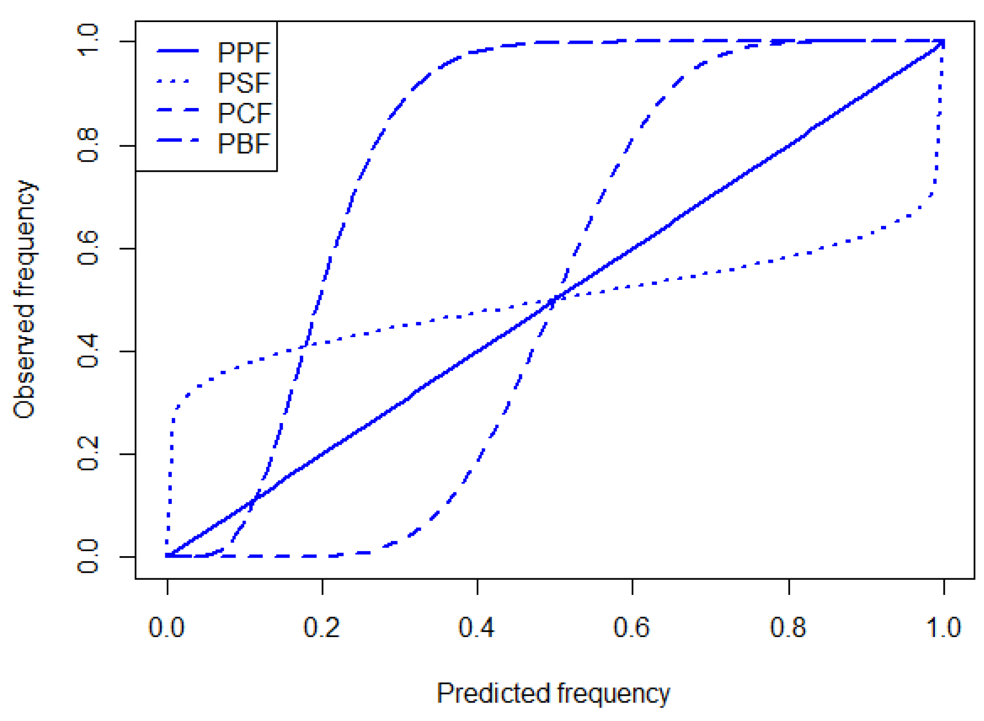
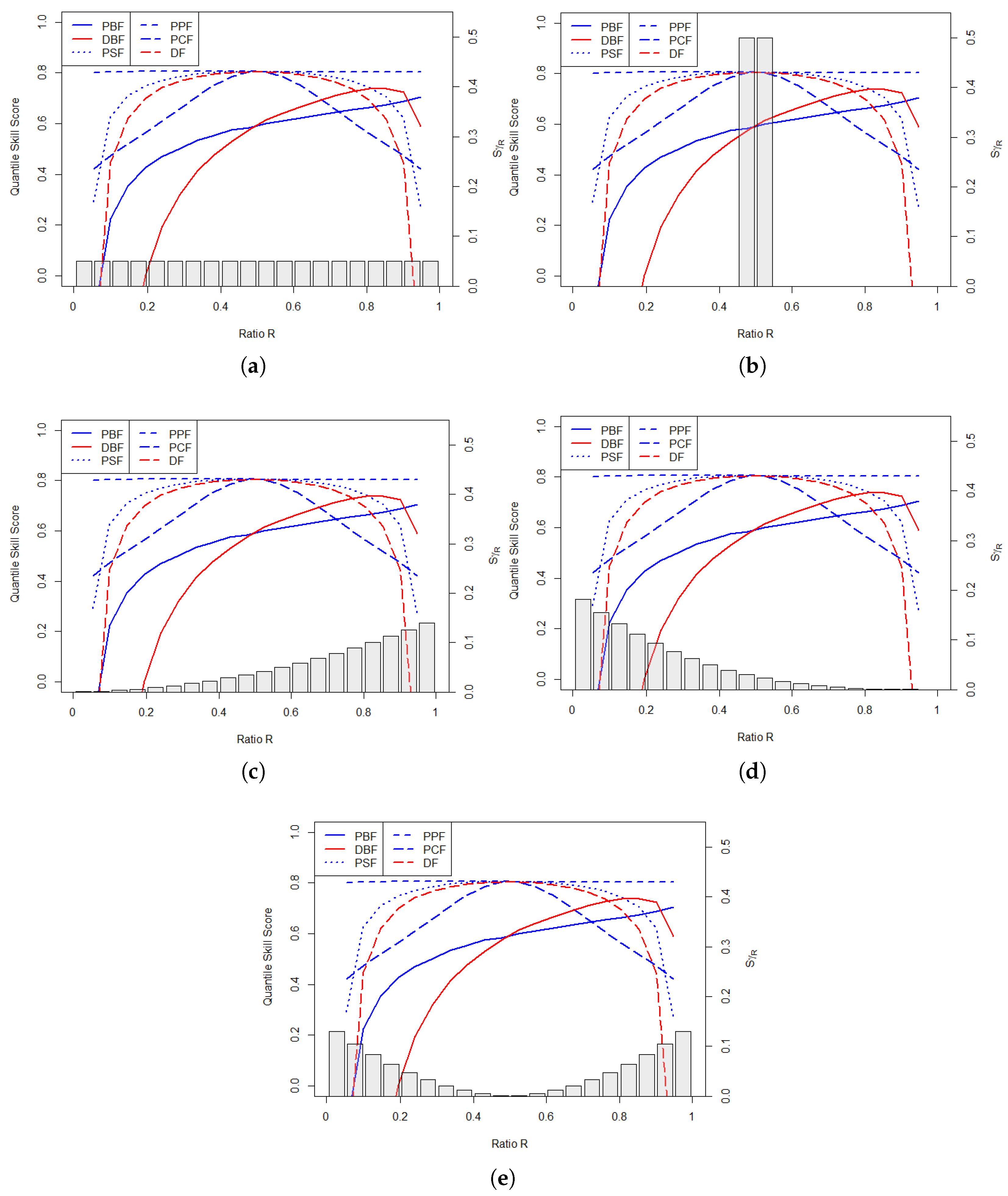
• A statistically consistent probabilistic forecast named “PPF” predicts $\mathcal{N}(X,20)$;
• A probabilistic sharp forecast named “PSF” predicts $\mathcal{N}(X,5)$;
• A probabilistic coarse forecast named “PCF” predicts $\mathcal{N}(X,70)$;
• A probabilistic unreliable (and biased) forecast named “PBF” predicts $\mathcal{N}(X,20)+\mathcal{U}(0,60)$, where $\mathcal{U}$ is uniform distribution;
• A deterministic unbiased forecast named “DF” predicts X;
• A deterministic biased forecast named “DBF” predicts $X+\mathcal{U}(0,60)$.

Appendix A shows some quality verification tools for probabilistic quality assessment (namely bias, sharpness and reliability diagrams) applied to these forecasts.

Quantile skill score diagrams for the different forecasts are plotted in Figure 7.

Obviously, the highest-performing forecast is the statistically consistent probabilistic forecast. All the other unbiased forecasts obtain comparable quantile skill scores for median ratios. However, deficiencies in sharpness (“PSF” or “PCF”) and deterministic forecasting result in performance drops for extreme ratios (close to 0 or 1). When the forecast (probabilistic or deterministic) is biased, the quantile skill score becomes asymmetric and decreases drastically for low ratios when the bias is positive. To understand how these differences translate into value in real decision-making scenarios, the effective value ($OEV$) of these forecasts was computed for several risk distributions, as presented below:

• The “Flat” distribution has uniform risks;
• The “Centered” distribution has only almost-symmetric ratios (close to 0.5);
• The “Right-Quad” distribution exhibits a prominence of high ratios;
• The “Left-Quad” distribution exhibits a prominence of small ratios;
• The “Ext-Quad” distribution avoids centered ratios.

The $EVC$ diagrams constructed for these study cases are presented in Figure 8.

For each risk distribution, a simulation of the decision-making process presented in Section 3 was conducted, and the quantitative results in terms of the OEV are presented in

Table 2. The effective values ($OEVs$) of the different forecasts for different risk distributions.

Risk Distribution
	Flat	Centered	Right-Quad	Left-Quad	Ext-Quad
PPF	80.4%	80.5%	80.4%	80.5%	80.4%
PSF	71.1%	80.5%	68.2%	68.7%	60.2%
PCF	62.9%	80.3%	60.3%	60.4%	52.4%
PBF	53.6%	59.2%	64.5%	39.9%	47.8%
DF	64.5%	80.5%	59.9%	60.3%	46.6%
DBF	46.7%	59.4%	65.4%	23.9%	38.2%

.

Again, the PPF consistently achieves the highest possible value across all risk distributions. The value of all the unbiased forecasts (“PSF”,“PCF”,“DF”) decreases strongly as soon as extreme ratios become prominent. This characteristic seems particularly significant for deterministic forecasting. Bias generally creates forecasts with relatively low values, even if it also makes them more unpredictable (see the high value of “DF” for the “Right-Quad” distribution).

6. Application to the Energy Market

This section proposes a simple example of a decision-making process in which forecasts of continuous variables can be used in practice and their value evaluated following the methodology detailed in Section 4.

6.1. Presentation of the Case Study

In this section, we study the value of the production forecast of a virtual solar power plant of 1 MWp for an operator selling their production on the day-ahead market for the year 2017 in several countries in Europe. In the majority of electricity markets, power plant managers are required to forecast their production. The selling price is fixed and the deviations are subject to linear penalties. Thus, market-based functions are appropriate to represent losses. Conveniently, the methodology exposed in Section 4.1 can be applied to assess the relative performances of deterministic and probabilistic forecasts. The slopes of the linear penalties are generally calculated a posteriori, according to rules defined by the grid manager, often linked with physical variables characterizing the state of the grid (imbalance, disponibility and costs of power reserves, etc.). We assume here that the imbalance prices (i.e., $S_1$ and $S_2$) are known in advance by the power plant operator. In reality, power plant managers often forecast the imbalance prices. As stated in Section 3.1, these forecasts are also operationally critical, as they determine the estimation of the risk ratio. Again, using probabilistic forecasts for the prices may lead to better decisions and increased gains [49].

For the purpose of this study, very simple deterministic and probabilistic forecasts have been constructed, with the help of the ensemble forecast of the European Centre of Medium-Range Weather Forecasts (ECMWF) Integrated Forecasting System (IFS). The predictions and measured irradiances have been converted into photovoltaic production according to the physical model described in [50]. The deterministic forecast is the ensemble mean, whereas the probabilistic forecast is the ensemble forecast, corrected by the variance deficit procedure [51]. A climatology forecast has also been created from historical data. To better demonstrate the EVC methodology, we selected three European countries with distinct imbalance price patterns: France, Portugal and Switzerland. The imbalance prices were downloaded from the online ENTSO-E Transparency platform [52].

6.2. Using the EVC Methodology

First, as noted in Section 4.1, the performances of the three forecasting models were evaluated with the quantile score diagram presented in Figure 9. The conclusions that arise are not surprising: the deterministic forecast performs almost identically whatever the quantile. On the contrary, probabilistic forecasting directs all its attention to extreme quantiles.

The EVC diagrams in Figure 10 clearly show the differences in penalty structures between the three different markets. Indeed, the risk distribution is clearly centered in the Portuguese market, is bimodal in the Swiss market and is characterized by the weight of extreme quantiles (0 and 1) in the French market. Following the EVC methodology, we can expect that the financial benefits brought by probabilistic forecasting should be limited in the Portuguese market and significant in the French market.

Table 3. The effective values ($OEVs$) of the two considered forecasts.

		Case
		France	Portugal	Switzerland
Forecast	Deterministic	4.7%	67.4%	55.0%
	Probabilistic	68.9%	69.7%	67.0%

presents the OEV of each model (i.e., the relative gains against the climatology, using Equation (9)).

As shown in Table 3, the probabilistic forecast is more valuable than the deterministic one for the three markets. In fact, this remains true regardless of the cost structure, as its quantile skill score is higher (or equal) for all probability levels. Notably, the quantile skill score of the two forecasts intersect at $R=0.5$, meaning that the median of the probabilistic forecast is just as effective as the deterministic forecast. Thus, all the added value arises from the probabilistic properties (sharpness and discrimination) that deterministic forecasts inherently lack. Considering the risk distribution diagrams of the three markets, it is clear that the more extreme the ratio is, the more benefits the probabilistic forecast provides. More importantly, contrary to the relative value of the deterministic forecast, the relative value of the probabilistic forecast remains stable between 65% and 70% across all markets, regardless of the risk distribution. In contrast, the quantile skill score of the deterministic forecast is strongly dependent on the dissymmetry ratio, so its effective value is very sensitive to the shape of the risk diagram. This is evident from the stark difference in performance between the French and Portuguese markets. This highlights an interesting feature of probabilistic forecasting: it offers robust value even when the cost structure is unknown or difficult to analyze in advance. However, this is not true for deterministic forecasting, for which the relative value is, in general, much more dependent on the cost structure. Importantly, these results assume that probabilistic information is used appropriately. Several studies have drawn attention to the misuse of probabilities: when poorly handled, probabilistic forecasts can lead to increased costs [53]. The effective communication of uncertainty and probabilistic information to end-users is therefore a crucial related topic [54,55].

7. Conclusions

In this work, we have proposed a new methodology to evaluate the value of forecasts of continuous variables for decision-making problems characterized by a piecewise linear loss function, also known as the market-based loss function. The methodology can be interpreted as an extension of a proven methodology used to assess the value of forecasts of binary events. We have shown the crucial roles of two indicators: $\gamma$, which represents the risk associated with one single decision, and the slope ratio R, which stands for the dissymmetry of the losses for the user. This methodology combines two graphical tools. First, the quantile skill score diagram represents the quality of the forecast. Second, the risk distribution diagram reflects the dissymmetry of the potential losses faced by the forecast user. We propose that the superimposition of these two graphical tools should be called the EVC (for the Effective economic Value of a forecast of a Continuous variable). An indicator named the OEV can also quantify the value of a forecast for a specific use case. We have found that, depending on the risk distribution, the superiority of probabilistic forecasts against deterministic forecasts can range from marginal (69.7% versus 67.4%) to considerable (68.9% versus 4.7%).

To illustrate the application of the EVC, we chose the financial optimization of a solar power plant operating across three European electricity markets, which constitutes a simple practical case. The substantial benefits provided by the probabilistic approach have been highlighted and quantified.

References

1. Clemen, R.T. Making Hard Decisions. Technometrics 2002, 44, 199–200. [Google Scholar] [CrossRef]
2. Thompson, J.C. On the Operational Deficiences in Categorical Weather Forecasts. Bull. Am. Meteorol. Soc. 1952, 33, 223–226. [Google Scholar] [CrossRef]
3. Sims, C. A Nine-Variable Probabilistic Macroeconomic Forecasting Model. In Business Cycles, Indicators, and Forecasting; National Bureau of Economic Research, Inc.: Cambridge, MA, USA, 1993; pp. 179–212. [Google Scholar]
4. Garratt, A.; Lee, K.; Pesaran, M.H.; Shin, Y. Forecast Uncertainties in Macroeconomic Modeling: An Application to the U.K. Economy. J. Am. Stat. Assoc. 2003, 98, 829–838. [Google Scholar] [CrossRef]
5. Chen, Z.; Iqbal, A.; Lai, H. Forecasting the probability of US recessions: A Probit and dynamic factor modelling approach. Can. J. Econ./Rev. Can. D’Econ. 2011, 44, 651–672. [Google Scholar] [CrossRef]
6. Forrest, D.; Simmons, R. Forecasting sport: The behaviour and performance of football tipsters. Int. J. Forecast. 2000, 16, 317–331. [Google Scholar] [CrossRef]
7. Bartos, J.A. The Assessment of Probability Distributions for Future Security Prices. Ph.D. Thesis, Indiana University, Bloomington, IN, USA, 1969. [Google Scholar]
8. Önkal, D.; Muradoglu, G. Effects of task format on probabilistic forecasting of stock prices. Int. J. Forecast. 1996, 12, 9–24. [Google Scholar] [CrossRef]
9. Adolfson, M.; Andersson, M.; Lindé, J.; Villani, M.; Vredin, A. Modern Forecasting Models in Action: Improving Macroeconomic Analyses at Central Banks. SSRN Electron. J. 2007, 829–838. [Google Scholar] [CrossRef]
10. Garratt, A.; Koop, G.; Mise, E.; Vahey, S.P. Real-Time Prediction With U.K. Monetary Aggregates in the Presence of Model Uncertainty. J. Bus. Econ. Stat. 2009, 27, 480–491. [Google Scholar] [CrossRef]
11. Schueller, G.I.; Gumbel, E.; Panggabean, H. Probabilistic determination of design wind velocity in Germany. Proc. Inst. Civ. Eng. 1976, 61, 673–683. [Google Scholar] [CrossRef]
12. Gel, Y.; Raftery, A.E.; Gneiting, T.; Tebaldi, C.; Nychka, D.; Briggs, W.; Roulston, M.S.; Berrocal, V.J. Calibrated Probabilistic Mesoscale Weather Field Forecasting: The Geostatistical Output Perturbation Method [with Comments, Rejoinder]. J. Am. Stat. Assoc. 2004, 99, 575–590. [Google Scholar] [CrossRef]
13. Gneiting, T.; Larson, K.; Westrick, K.; Genton, M.; Aldrich, E. Calibrated Probabilistic Forecasting at the Stateline Wind Energy Center: The Regime-Switching SpaceTime Method. J. Am. Stat. Assoc. 2006, 101, 968–979. [Google Scholar] [CrossRef]
14. Murphy, A.H.; Winkler, R.L. Probability Forecasting in Meterology. J. Am. Stat. Assoc. 1984, 79, 489–500. [Google Scholar] [CrossRef]
15. Sloughter, J.M.; Gneiting, T.; Raftery, A. Probabilistic Wind Speed Forecasting Using Ensembles and Bayesian Model Averaging. J. Am. Stat. Assoc. 2010, 105, 25–35. [Google Scholar] [CrossRef]
16. Gneiting, T.; Raftery, A.E. Strictly Proper Scoring Rules, Prediction, and Estimation. J. Am. Stat. Assoc. 2007, 102, 359–378. [Google Scholar] [CrossRef]
17. Roulston, M.S.; Smith, L.A. Evaluating Probabilistic Forecasts Using Information Theory. Mon. Weather Rev. 2002, 130, 1653–1660. [Google Scholar] [CrossRef]
18. Murphy, A.H. What Is a Good Forecast? An Essay on the Nature of Goodness in Weather Forecasting. Weather Forecast. 1993, 8, 281–293. [Google Scholar] [CrossRef]
19. Zhu, Y.; Toth, Z.; Wobus, R.; Richardson, D.; Mylne, K. The economic value of ensemble-based weather forecasts. Bull. Am. Meteorol. Soc. 2002, 83, 73–83. [Google Scholar] [CrossRef]
20. Wilks, D.S.; Hamill, T.M. Potential Economic Value of Ensemble-Based Surface Weather Forecasts. Mon. Weather Rev. 1995, 123, 3565–3575. [Google Scholar] [CrossRef]
21. Gneiting, T.; Katzfuss, M. Probabilistic Forecasting. Annu. Rev. Stat. Its Appl. 2014, 1, 125–151. [Google Scholar] [CrossRef]
22. Thompson, J.C.; Brier, G.W. The economic utility of weather forecasts. Mon. Weather Rev. 1955, 83, 249–253. [Google Scholar] [CrossRef]
23. Murphy, A.H. A Note on the Utility of Probabilistic Predictions and the Probability Score in the Cost-Loss Ratio Decision Situation. J. Appl. Meteorol. Climatol. 1966, 5, 534–537. [Google Scholar] [CrossRef]
24. Murphy, A.H. The Value of Climatological, Categorical and Probabilistic Forecasts in the Cost-Loss Ratio Situation. Mon. Weather Rev. 1977, 105, 803–816. [Google Scholar] [CrossRef]
25. Murphy, A.H. Hedging and the Mode of Expression of Weather Forecasts. Bull. Am. Meteorol. Soc. 1978, 59, 371–373. [Google Scholar] [CrossRef]
26. Thornes, J.; Stephenson, D. How to judge the quality and value of weather forecast products. Meteorol. Appl. 2001, 8, 307–314. [Google Scholar] [CrossRef]
27. Wilks, D.S. A skill score based on economic value for probability forecasts. Meteorol. Appl. 2001, 8, 209–219. [Google Scholar] [CrossRef]
28. Buizza, R. The value of probabilistic prediction. Atmos. Sci. Lett. 2008, 9, 36–42. [Google Scholar] [CrossRef]
29. Richardson, D.S. Skill and relative economic value of the ECMWF ensemble prediction system. Q. J. R. Meteorol. Soc. 2000, 126, 649–667. [Google Scholar] [CrossRef]
30. Mylne, K.R. Decision-making from probability forecasts based on forecast value. Meteorol. Appl. 2002, 9, 307–315. [Google Scholar] [CrossRef]
31. Smith, L.; S., R.M.; von Hardenbergm, J. End to End Ensemble Forecasting: Towards Evaluating the Economic Value of the Ensemble Prediction System; Technical Memorandum; European Centre for Medium-Range Weather Forecasts: Reading, UK, 2001. [Google Scholar]
32. Roulston, M.S.; Kaplan, D.T.; von Hardenberg, J.; Smith, L.A. Using medium-range weather forcasts to improve the value of wind energy production. Renew. Energy 2003, 28, 585–602. [Google Scholar] [CrossRef]
33. Pinson, P.; Chevallier, C.; Kariniotakis, G. Optimizing Benefits from wind power participation in electricity market using advanced tools for wind power forecasting and uncertainty assessment. In Proceedings of the EWEC 2004, London, UK, 22–25 November 2004. [Google Scholar]
34. Murphy, A.H.; Katz, R.W.; Winkler, R.L.; Hsu, W. Repetitive decision making and the value of forecasts in the cost-loss ratio situation: A dynamic model. Mon. Weather Rev. 1985, 113, 801–813. [Google Scholar] [CrossRef]
35. Buizza, R. Accuracy and Potential Economic Value of Categorical and Probabilistic Forecasts of Discrete Events. Mon. Weather Rev. 2001, 129, 2329–2345. [Google Scholar] [CrossRef]
36. Doubleday, K.; Van Scyoc Hernandez, V.; Hodge, B. Benchmark probabilistic solar forecasts: Characteristics and recommendations. Sol. Energy 2020, 206, 52–67. [Google Scholar] [CrossRef]
37. Le Gal La Salle, J.; David, M.; Lauret, P. A new climatology reference model to benchmark probabilistic solar forecasts. Sol. Energy 2021, 223, 398–414. [Google Scholar] [CrossRef]
38. Wilks, D. Statistical Methods in the Atmospheric Sciences; Academic Press: Cambridge, MA, USA, 2014. [Google Scholar]
39. Ramahatana, F.; David, M. Economic optimization of micro-grid operations by dynamic programming with real energy forecast. J. Phys. Conf. Ser. 2019, 1343, 012067. [Google Scholar] [CrossRef]
40. Holttinen, H. Optimal electricity market for wind power. Energy Policy 2005, 33, 2052–2063. [Google Scholar] [CrossRef]
41. Linnet, U. Tools Supporting Wind Energy Trade in Deregulated Markets. Ph.D. Thesis, Technical University of Denmark, Lyngby, Denmark, 2005. [Google Scholar]
42. Pinson, P.; Chevallier, C.; Kariniotakis, G. Trading Wind Generation from Short-Term Probabilistic Forecasts of Wind Power. IEEE Trans. Power Syst. 2007, 22, 1148–1156. [Google Scholar] [CrossRef]
43. Lauret, P.; David, M.; Pinson, P. Verification of solar irradiance probabilistic forecasts. Sol. Energy 2019, 194, 254–271. [Google Scholar] [CrossRef]
44. Benedetti, R. Scoring Rules for Forecast Verification. Mon. Weather Rev. 2010, 138, 203–211. [Google Scholar] [CrossRef]
45. Selten, R. Axiomatic Characterization of the Quadratic Scoring Rule. Exp. Econ. 1998, 1, 43–61. [Google Scholar] [CrossRef]
46. Bentzien, S.; Friederichs, P. Decomposition and graphical portrayal of the quantile score: Quantile Score Decomposition and Portrayal. Q. J. R. Meteorol. Soc. 2014, 140, 1924–1934. [Google Scholar] [CrossRef]
47. Ben Bouallègue, Z.; Pinson, P.; Friederichs, P. Quantile forecast discrimination ability and value. Q. J. R. Meteorol. Soc. 2015, 141, 3415–3424. [Google Scholar] [CrossRef]
48. Gneiting, T.; Ranjan, R. Comparing Density Forecasts Using Threshold- and Quantile-Weighted Scoring Rules. J. Bus. Econ. Stat. 2011, 29, 411–422. [Google Scholar] [CrossRef]
49. Lipiecki, A.; Uniejewski, B.; Weron, R. Postprocessing of Point Predictions for Probabilistic Forecasting of Day-Ahead Electricity Prices: The Benefits of Using Isotonic Distributional Regression. Energy Econ. 2024, 139, 107934. [Google Scholar] [CrossRef]
50. Luque, A.; Hegedus, S. Handbook of Photovoltaic Science and Engineering; Wiley: Chichester, UK, 2011. [Google Scholar]
51. Alessandrini, S.; Sperati, S.; Pinson, P. A comparison between the ECMWF and COSMO Ensemble Prediction Systems applied to short-term wind power forecasting on real data. Appl. Energy 2013, 107, 271–280. [Google Scholar] [CrossRef]
52. ENTSO-E. Transparency Platform. Available online: https://transparency.entsoe.eu (accessed on 1 April 2025).
53. Sivle, A.D.; Agersten, S.; Schmid, F.; Simon, A. Use and perception of weather forecast information across Europe. Meteorol. Appl. 2022, 29, e2053. [Google Scholar] [CrossRef]
54. van der Bles, A.M.; van der Linden, S.; Freeman, A.; Mitchell, J.; Galvao, A.; Zaval, L.; Spiegelhalter, D. Communicating uncertainty about facts, numbers and science. R. Soc. Open Sci. 2019, 6, 181870. [Google Scholar] [CrossRef] [PubMed]
55. Spiegelhalter, D. Risk and uncertainty communication. Annu. Rev. Stat. Its Appl. 2017, 4, 31–60. [Google Scholar] [CrossRef]
56. Bröcker, J.; Smith, L.A. Increasing the Reliability of Reliability Diagrams. Weather Forecast. 2007, 22, 651–661. [Google Scholar] [CrossRef]
Figure 1. An example of a cost diagram.
Forecasting 07 00030 g001
Figure 2. The compared values of a probabilistic forecast (“EPS”) and a deterministic forecast (“control”). Based on Buizza’s work [28] and reproduced with permission from John Wiley & Sons.
Forecasting 07 00030 g002
Figure 3. An example of a market-based loss function.
Forecasting 07 00030 g003
Figure 4. Examples of a quantile score diagram and a quantile skill score diagram. (a) A quantile score diagram. (b) A quantile skill score (or PEVC) diagram.
Forecasting 07 00030 g004
Figure 5. An example of a risk distribution diagram.
Forecasting 07 00030 g005
Figure 6. Construction of an EVC diagram.
Forecasting 07 00030 g006
Figure 7. Quantile skill score diagrams for the studied forecasts. (a) Non-biased forecasts. (b) Biased forecasts.
Forecasting 07 00030 g007
Figure 8. EVC diagrams of the considered forecasts for the selected risk distributions. (a) Flat distribution. (b) Centered distribution. (c) Right-Quad distribution. (d) Left-Quad distribution. (e) Ext-Quad distribution.
Forecasting 07 00030 g008
Figure 9. The quantile score diagrams of the three forecasting models.
Forecasting 07 00030 g009
Figure 10. The EVC diagrams of the three selected markets. (a) France. (b) Portugal. (c) Switzerland.
Forecasting 07 00030 g010