

Parallel Multi-Model Energy Demand Forecasting with Cloud Redundancy: Leveraging Trend Correction, Feature Selection, and Machine Learning


Abstract
1. Introduction
- (a)
- Hybrid forecasting framework with deviation correction:
- (b)
- Fault Tolerance via Distributed Cloud Deployment and Voting:
- (c)
- Generalizable and Adaptable Methodology
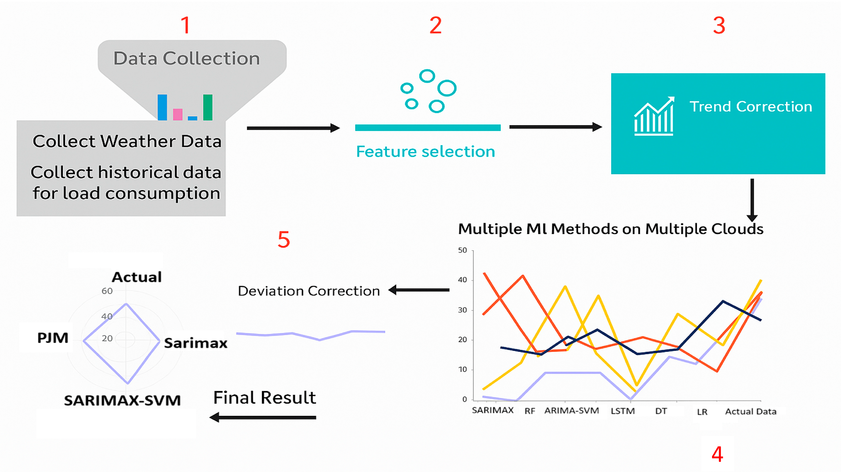
2. Methodology
2.1. Procedures
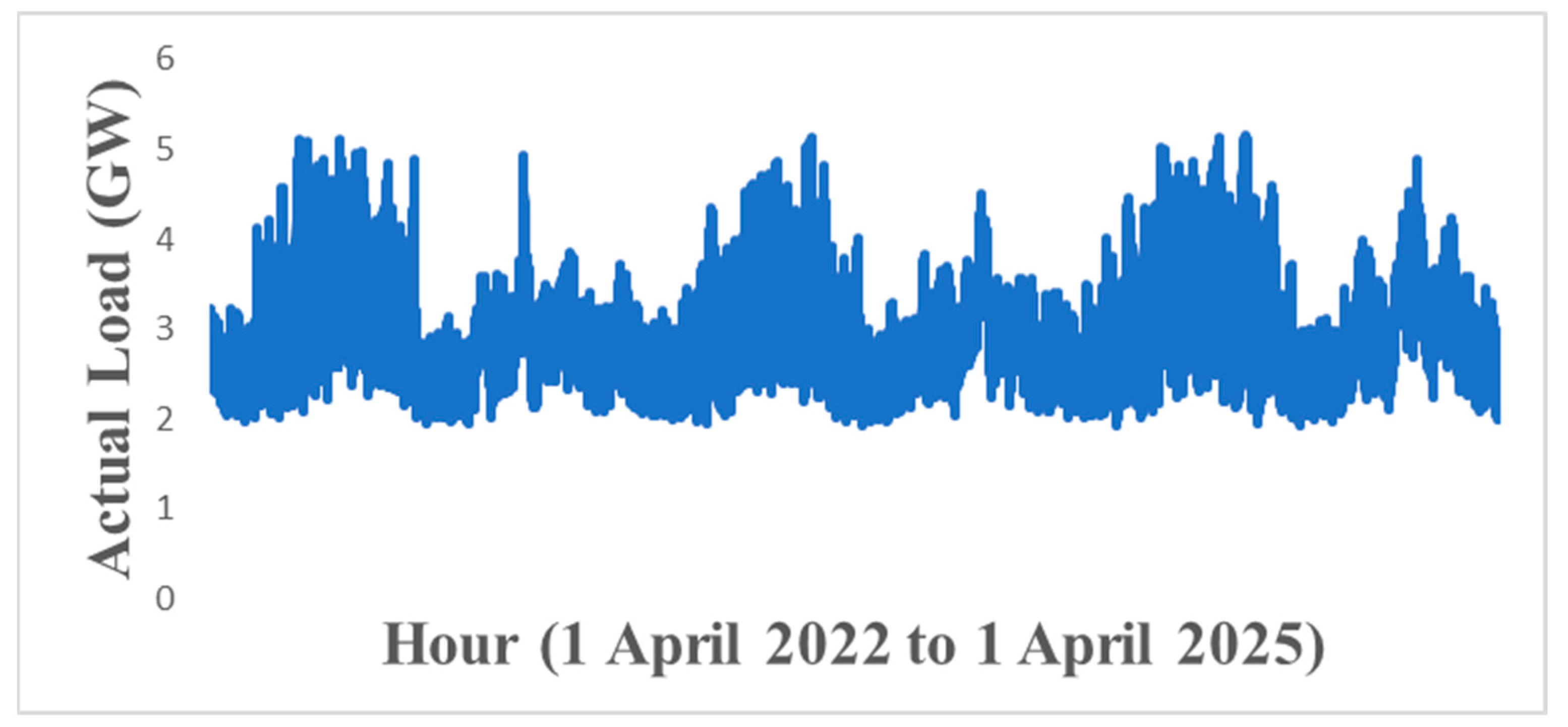
2.2. 1-Collecting Historical Data for Load Consumption
2.3. 2-Feature Selection
Correlation Matrix (CM)
- +1: means that the two variables increase proportionally as one increases.
- −1: indicates that a perfect negative correlation exists, meaning that as one variable increases, the other variable decreases proportionally.
- A correlation of 0: there is no linear relationship between the variables. It is still possible; however, that another nonlinear relationship exists.
2.4. 3-Trend Correction
2.5. Implementation of Multiple Machine Learning Methods on Multiple Clouds
2.6. Deviation Correction (DC)
Description 1: Parameters of the Proposed Model
- Input:
- Dataset D from 1 April 2022, to 30 March 2025;
- Forecast horizon: next 24 h (31 March 2025).
- Output:
- Hourly load forecast for 31 March 2025, with refined predictions for the first 5 h of 1 April 2025.
- Data Partitioning
- 24 h Forecasting
- 2.1.
- Train the forecasting models on the training set.
- 2.2.
- Generate the forecast for the next 29 h: 24 h for 31 March 2025 (A), and the first 5 h of 1 April 2025 (B).
- Deviation Analysis and Correction
- 3.1.
- Analyze the deviation trend within the test set.
- 3.2.
- Forecast the deviation for the first 5 h of 1 April 2025 (C).
- 3.3.
- For the first 5 h, compute the corrected forecast:
- Final Forecast = B + C
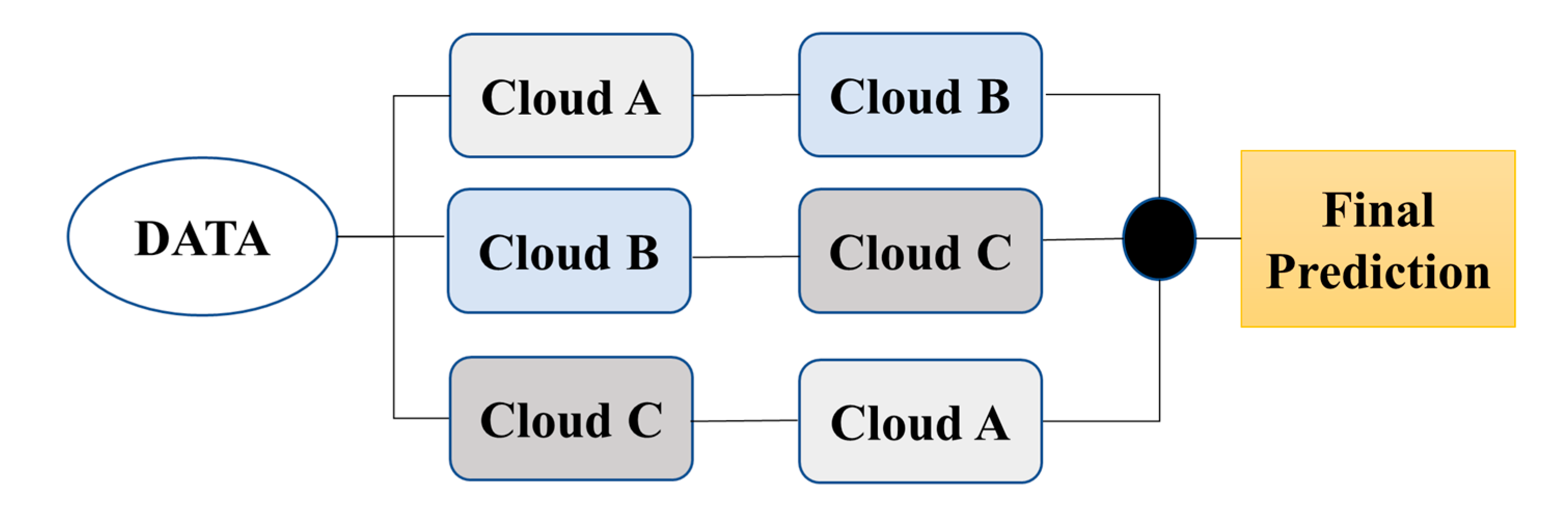
- Fault Tolerance via 2-out-of-3 Voting on Three Cloud Platforms
- 4.1.
- Deploy three different models on three cloud platforms.
- 4.2.
- Determine the final prediction by majority voting (averaging the consensus) if at least two out of the three platforms produce consistent predictions.
- R represents reliability.
3. Results
4. Discussion
5. Conclusions
Author Contributions
Funding
Data Availability Statement
Conflicts of Interest
Nomenclature
| Metric | Definition |
| MSE | Mean square error |
| MAE | Mean absolute error |
| MAPE | Mean absolute percentage error |
| RMSE | Root mean square error |
| AE | Average error |
| DC | Deviation correction |
| ML | Machine learning |
| SARIMAX | Seasonal autoregressive integrated moving average with exogenous regressors |
| DT | Decision tree |
| LSTM | Long short-term memory |
| SVM | Support vector machine |
| LR | Linear regression |
| ANN | Artificial neural networks |
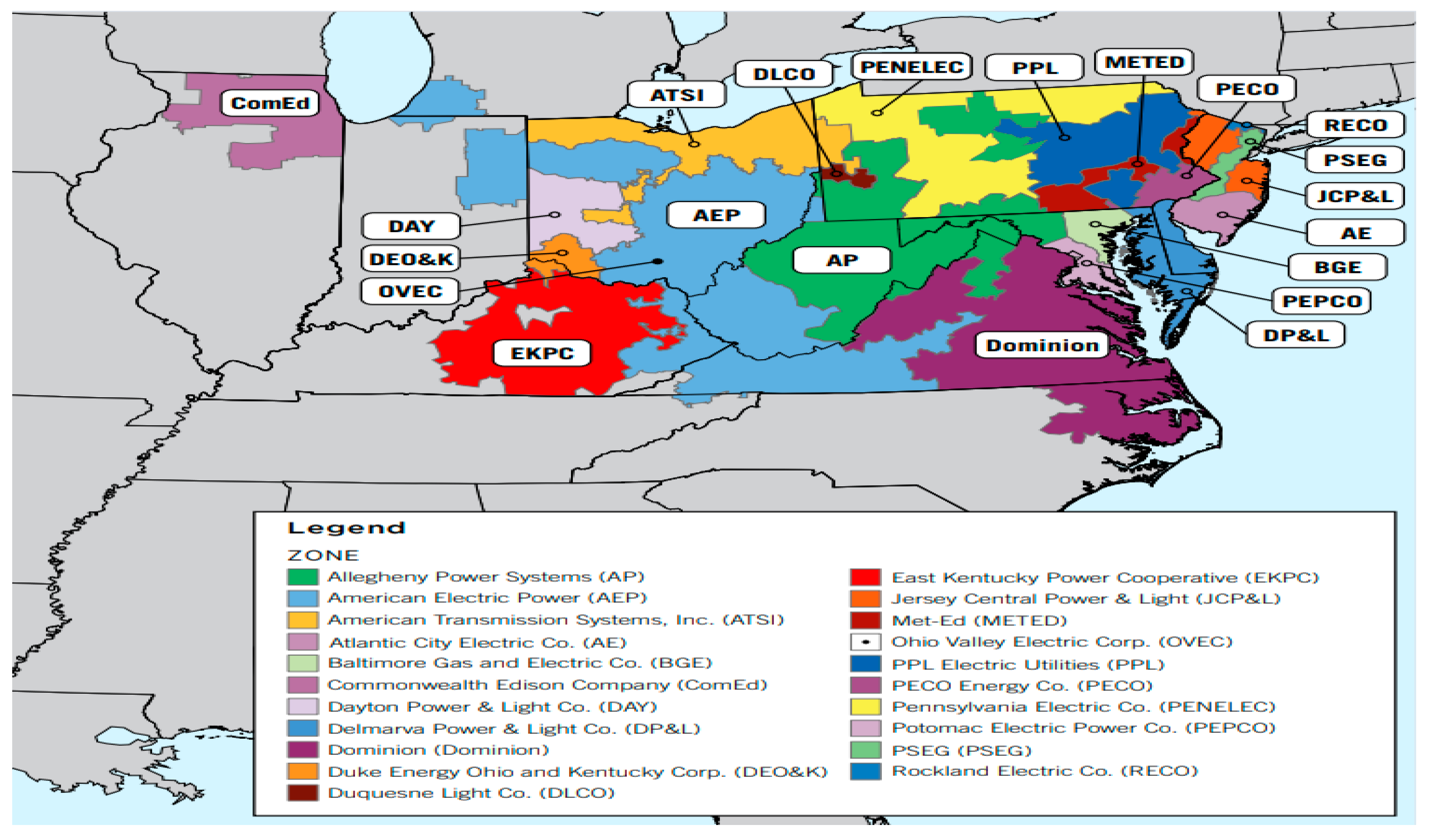
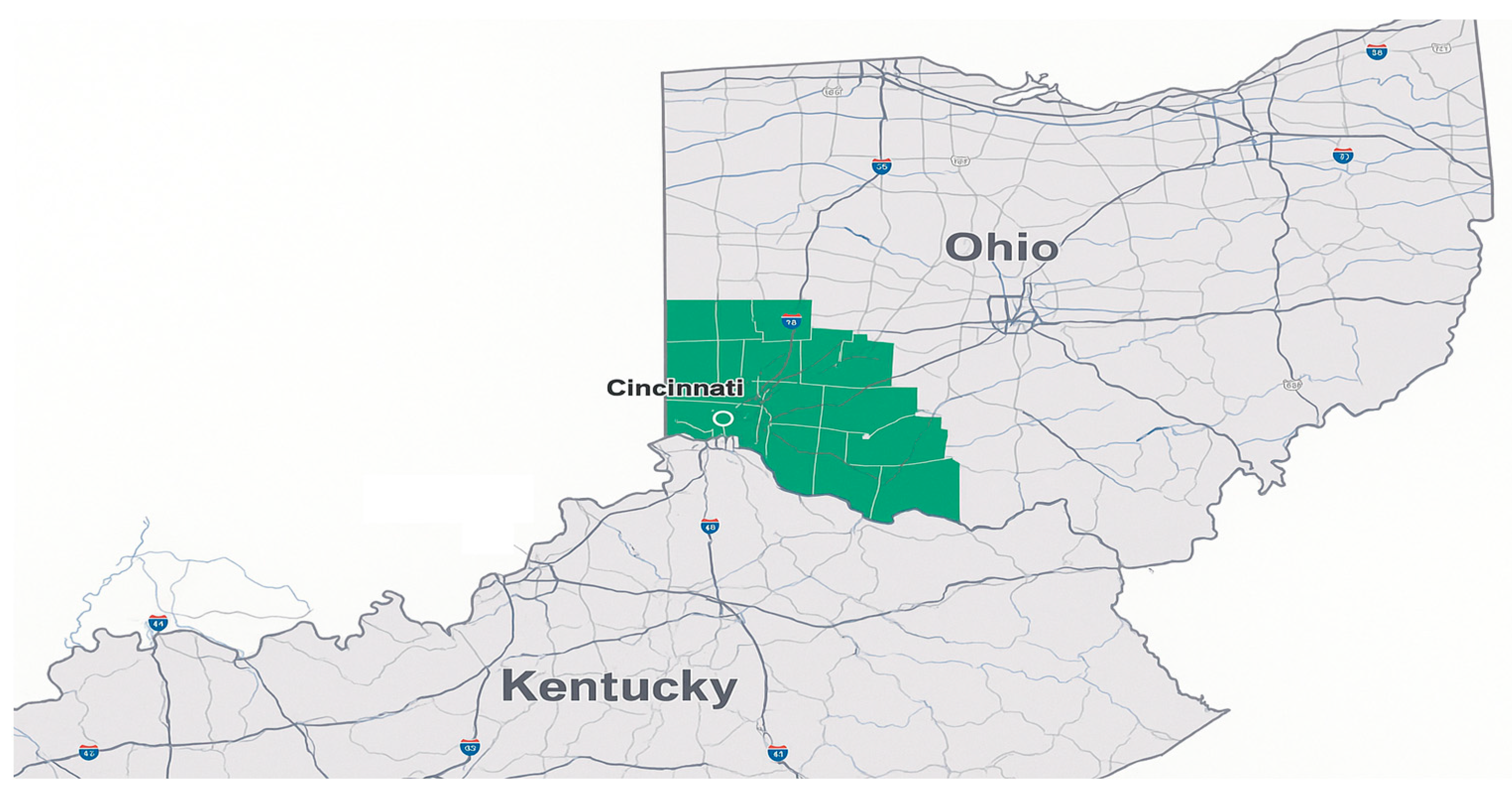
| DEO&K Co | Duke Energy Ohio and Kentucky |
| TC | Trend correction |
| AWS | Amazon Web Services |
| CM | Correlation matrix |
| PJM | PJM is a regional transmission organization (RTO) that coordinates the movement of wholesale electricity in all or parts of 13 states and the District of Columbia |
References
- Chou, J.-S.; Tran, D.-S. Forecasting Energy Consumption Time Series Using Machine Learning Techniques Based on Usage Patterns of Residential Householders. Energy 2018, 165, 709–726. [Google Scholar] [CrossRef]
- Baesmat, K.H.; Shiri, A. A New Combined Method for Future Energy Forecasting in Electrical Networks. Int. Trans. Electr. Energy Syst. 2019, 29, e2749. [Google Scholar] [CrossRef]
- Baesmat, K.H.; Masoudipour, I.; Samet, H. Improving the Performance of Short-Term Load Forecast Using a Hybrid Artificial Neural Network and Artificial Bee Colony Algorithm. IEEE Can. J. Electr. Comput. Eng. 2021, 44, 275–282. [Google Scholar] [CrossRef]
- Singh, U.; Rizwan, M.; Alaraj, M.; Alsaidan, I. A Machine Learning-Based Gradient Boosting Regression Approach for Wind Power Production Forecasting: A Step towards Smart Grid Environments. Energies 2021, 14, 5196. [Google Scholar] [CrossRef]
- Haq, E.U.; Lyu, X.; Jia, Y.; Hua, M.; Ahmad, F. Forecasting Household Electric Appliances Consumption and Peak Demand Based on Hybrid Machine Learning Approach. Energy Rep. 2020, 6 (Suppl. 9), 1099–1105. [Google Scholar] [CrossRef]
- Baesmat, K.H.; Shokoohi, F.; Farrokhi, Z. SP-RF-ARIMA: A sparse random forest and ARIMA hybrid model for electric load forecasting. Glob. Energy Interconnect. in press. 2025. [Google Scholar] [CrossRef]
- Ahmad, T.; Chen, H.; Zhang, D.; Zhang, H. Smart Energy Forecasting Strategy with Four Machine Learning Models for Climate-Sensitive and Non-Climate-Sensitive Conditions. Energy 2020, 198, 117283. [Google Scholar] [CrossRef]
- Khan, P.W.; Byun, Y.-C. Genetic Algorithm Based Optimized Feature Engineering and Hybrid Machine Learning for Effective Energy Consumption Prediction. IEEE Access 2020, 8, 196274–196286. [Google Scholar] [CrossRef]
- Torabi, M.; Hashemi, S.; Saybani, M.; Shamshirband, S.; Mosavi, A. A Hybrid Clustering and Classification Technique for Forecasting Short-Term Energy Consumption. Environ. Prog. Sustain. Energy 2018, 38, 66–76. [Google Scholar] [CrossRef]
- Deb, C.; Zhang, F.; Yang, J.; Lee, S.; Shah, K. A Review on Time Series Forecasting Techniques for Building Energy Consumption. Renew. Sustain. Energy Rev. 2017, 74, 902–924. [Google Scholar] [CrossRef]
- Chou, J.-S.; Ngo, N.-T. Time Series Analytics Using Sliding Window Metaheuristic Optimization-Based Machine Learning System for Identifying Building Energy Consumption Patterns. Appl. Energy 2016, 177, 751–770. [Google Scholar] [CrossRef]
- Dong, B.; Cao, C.; Lee, S.E. Applying Support Vector Machines to Predict Building Energy Consumption in Tropical Region. Energy Build. 2005, 37, 545–553. [Google Scholar] [CrossRef]
- Mawson, V.J.; Hughes, B.R. Deep Learning Techniques for Energy Forecasting and Condition Monitoring in the Manufacturing Sector. Energy Build. 2020, 217, 109966. [Google Scholar] [CrossRef]
- Persson, C.; Bacher, P.; Shiga, T.; Madsen, H. Multi-Site Solar Power Forecasting Using Gradient Boosted Regression Trees. Sol. Energy 2017, 150, 423–436. [Google Scholar] [CrossRef]
- Bogner, K.; Pappenberger, F.; Zappa, M. Machine Learning Techniques for Predicting the Energy Consumption/Production and Its Uncertainties Driven by Meteorological Observations and Forecasts. Sustainability 2019, 11, 3328. [Google Scholar] [CrossRef]
- Hong, T.; Wang, P.; White, L. Weather station selection for electric load forecasting. Int. J. Forecast. 2015, 31, 286–295. [Google Scholar] [CrossRef]
- Jain, R.; Smith, K.; Culligan, P.; Taylor, J. Forecasting Energy Consumption of Multi-Family Residential Buildings Using Support Vector Regression: Investigating the Impact of Temporal and Spatial Monitoring Granularity on Performance Accuracy. Appl. Energy 2014, 123, 168–178. [Google Scholar] [CrossRef]
- Ma, J.; Oppong, A.; Acheampong, K.N.; Abruquah, L.A. Forecasting Renewable Energy Consumption under Zero Assumptions. Sustainability 2018, 10, 576. [Google Scholar] [CrossRef]
- Abdel-Aal, R.E.; Al-Garni, A.Z.; Al-Nassar, Y.N. Modelling and Forecasting Monthly Electric Energy Consumption in Eastern Saudi Arabia Using Abductive Networks. Energy 1997, 22, 911–921. [Google Scholar] [CrossRef]
- Ahmad, T.; Chen, H.; Huang, R.; Guo, Y.; Wang, J.; Shair, J.; Akram, H.M.A.; Mohsan, S.A.H.; Kazim, M. Supervised Based Machine Learning Models for Short-, Medium- and Long-Term Energy Prediction in Distinct Building Environments. Energy 2018, 158, 17–32. [Google Scholar] [CrossRef]
- Shin, S.; Woo, H. Energy Consumption Forecasting in Korea Using Machine Learning Algorithms. Energies 2022, 15, 4880. [Google Scholar] [CrossRef]
- Bourdeau, M.; Zhai, X.-Q.; Nefzaoui, E.; Guo, X.; Chatellier, P. Modeling and Forecasting Building Energy Consumption: A Review of Data-Driven Techniques. Sustain. Cities Soc. 2019, 48, 101533. [Google Scholar] [CrossRef]
- Lin, X.; Yu, H.; Wang, M.; Li, C.; Wang, Z.; Tang, Y. Electricity Consumption Forecast of High-Rise Office Buildings Based on the Long Short-Term Memory Method. Energies 2021, 14, 4785. [Google Scholar] [CrossRef]
- Demolli, H.; Dokuz, A.S.; Ecemis, A.; Gokcek, M. Wind Power Forecasting Based on Daily Wind Speed Data Using Machine Learning Algorithms. Energy Convers. Manag. 2019, 198, 111823. [Google Scholar] [CrossRef]
- Herrera, G.P.; Constantino, M.; Miranda Tabak, B.; Pistori, H.; Su, J.-J. Long-Term Forecast of Energy Commodities Price Using Machine Learning. Energy 2019, 179, 214–221. [Google Scholar] [CrossRef]
- Wei, N.; Li, C.; Peng, X.; Zeng, F.; Lu, X. Conventional Models and Artificial Intelligence-Based Models for Energy Consumption Forecasting: A Review. J. Pet. Sci. Eng. 2019, 181, 106187. [Google Scholar] [CrossRef]
- Beyca, O.; Ervural, B.; Tatoğlu, E.; Ozuyar, P.; Zaim, S. Using Machine Learning Tools for Forecasting Natural Gas Consumption in the Province of Istanbul. Energy Econ. 2019, 20, 937–949. [Google Scholar] [CrossRef]
- Baesmat, K.H. Impedance Analysis of Adaptive Distance Relays Using Machine Learning. In ITNG 2024: 21st International Conference on Information Technology-New Generations; Latifi, S., Ed.; Advances in Intelligent Systems and Computing; Springer: Cham, Switzerland, 2024; Volume 1456. [Google Scholar] [CrossRef]
- Khan, P.W.; Kim, Y.; Byun, Y.-C.; Lee, S.-J. Influencing Factors Evaluation of Machine Learning-Based Energy Consumption Prediction. Energies 2021, 14, 7167. [Google Scholar] [CrossRef]
- Divina, F.; García Torres, M.; Goméz Vela, F.A.; Vázquez Noguera, J.L. A Comparative Study of Time Series Forecasting Methods for Short Term Electric Energy Consumption Prediction in Smart Buildings. Energies 2019, 12, 1934. [Google Scholar] [CrossRef]
- Nizami, S.J.; Al-Garni, A.Z. Forecasting Electric Energy Consumption Using Neural Networks. Energy Policy 1995, 23, 1097–1104. [Google Scholar] [CrossRef]
- Khan, P.W.; Byun, Y.-C.; Lee, S.-J.; Park, N. Machine Learning Based Hybrid System for Imputation and Efficient Energy Demand Forecasting. Energies 2020, 13, 2681. [Google Scholar] [CrossRef]
- Hafeez, G.; Alimgeer, K.; Khan, I. Electric Load Forecasting Based on Deep Learning and Optimized by Heuristic Algorithm in Smart Grid. Appl. Energy 2020, 269, 114915. [Google Scholar] [CrossRef]
- Ahmad, T.; Chen, H. A Review on Machine Learning Forecasting Growth Trends and Their Real-Time Applications in Different Energy Systems. Sustain. Cities Soc. 2020, 54, 102010. [Google Scholar] [CrossRef]
- Hou, W.; Wen, H.; Zhang, N.; Lei, W.; Lin, H. Dynamic Load Combined Prediction Framework with Collaborative Cloud-Edge for Microgrid. In Proceedings of the IEEE Conference on Computer Communications Workshops (INFOCOM WKSHPS), New York, NY, USA, 2–5 May 2022; pp. 1–2. [Google Scholar] [CrossRef]
- Zhang, X.; Zeng, Z.; Wang, P.; Song, J.; Kong, Z. A Hybrid Edge-Cloud Computing Method for Short-Term Electric Load Forecasting Based on Smart Metering Terminal. In Proceedings of the 2020 IEEE 4th Conference on Energy Internet and Energy System Integration (EI2 2020), Wuhan, China, 30 October–1 November 2020; pp. 3101–3105. [Google Scholar] [CrossRef]
- Raju, M.; Laxmi, A. IOT Based Online Load Forecasting Using Machine Learning Algorithms. Procedia Comput. Sci. 2020, 171, 551–560. [Google Scholar] [CrossRef]
- Geberslassie, M.; Bitzer, B. Cloud Computing for Renewable Power Systems. Renew. Energy Power Qual. 2012, 10, 1250–1254. [Google Scholar] [CrossRef]
- Hou, S.; Li, H.; Yang, C.; Wang, L. A New Privacy-Preserving Framework Based on Edge-Fog-Cloud Continuum for Load Forecasting. In Proceedings of the 2020 IEEE Wireless Communications and Networking Conference (WCNC), Seoul, Republic of Korea, 25–28 May 2020; pp. 1–8. [Google Scholar] [CrossRef]
- Pelluri, S.; Srinivas, P.; Sneha, S. A Compendium on Load Forecasting Approaches and Models. Int. J. Res. Eng. Technol. 2014, 3, 27–36. [Google Scholar] [CrossRef]
- Devaraj, J.; Madurai Elavarasan, R.; Shafiullah, G.; Jamal, T.; Khan, I. A Holistic Review on Energy Forecasting Using Big Data and Deep Learning Models. Int. J. Energy Res. 2021, 45, 13489–13530. [Google Scholar] [CrossRef]
- PJM Website. Available online: https://www.pjm.com/ (accessed on 21 May 2025).
- Baesmat, K.H.; Latifi, S. A New Hybrid Method for Electrical Load Forecasting Based on Deviation Correction and MRMRMS. In Proceedings of the 30th International Conference on Systems Engineering, ICSEng 2023, Las Vegas, NV, USA, 22–24 August 2023; Volume 761. [Google Scholar] [CrossRef]
- Zeinab, F.; Kalhor, A.; Tale Masouleh, M. Implementation and Evaluation of Object Identification Techniques on Nao Robot Platform. Int. J. Mechatron. Electr. Comput. Technol. 2018, 8, 3947–3958. Available online: https://aeuso.org/includes/files/articles/Vol8_Iss29_3947-3958_Implementation_and_Evaluation_of_Ob.pdf (accessed on 21 May 2025).
- Farrokhi, Z.; Baesmat, K.; Regentova, E. Enhancing Urban Intelligence Energy Management: Innovative Load Forecasting Techniques for Electrical Networks. J. Power Energy Eng. 2024, 12, 72–88. [Google Scholar] [CrossRef]
- Zielińska-Sitkiewicz, M.; Chrzanowska, M.; Furmańczyk, K.; Paczutkowski, K. Analysis of Electricity Consumption in Poland Using Prediction Models and Neural Networks. Energies 2021, 14, 6619. [Google Scholar] [CrossRef]
- Gajdzik, B.; Wolniak, R.; Nagaj, R.; Žuromskaitė-Nagaj, B.; Grebski, W.W. The Influence of the Global Energy Crisis on Energy Efficiency: A Comprehensive Analysis. Energies 2024, 17, 947. [Google Scholar] [CrossRef]
- Elhaby, K.; Baina, A.; Bellafkih, M.; Deifalla, A.F. Machine Learning Algorithms for Predicting Energy Consumption in Educational Buildings. Int. J. Energy Res. 2024, 1, 6812425. [Google Scholar] [CrossRef]


| Features | Correlation Value | Features | Correlation Value |
|---|---|---|---|
| Dispatch rate | 0.33921 | Condition | −0.029156 |
| Wind Speed | 0.11236 | Pressure | −0.091274 |
| Wind Gust | 0.11188 | Dew Point | −0.10462 |
| Humidity | 0.052206 | Temperature | −0.1339 |
| Precipitation | 0.0035134 | Actual Load | 1 |
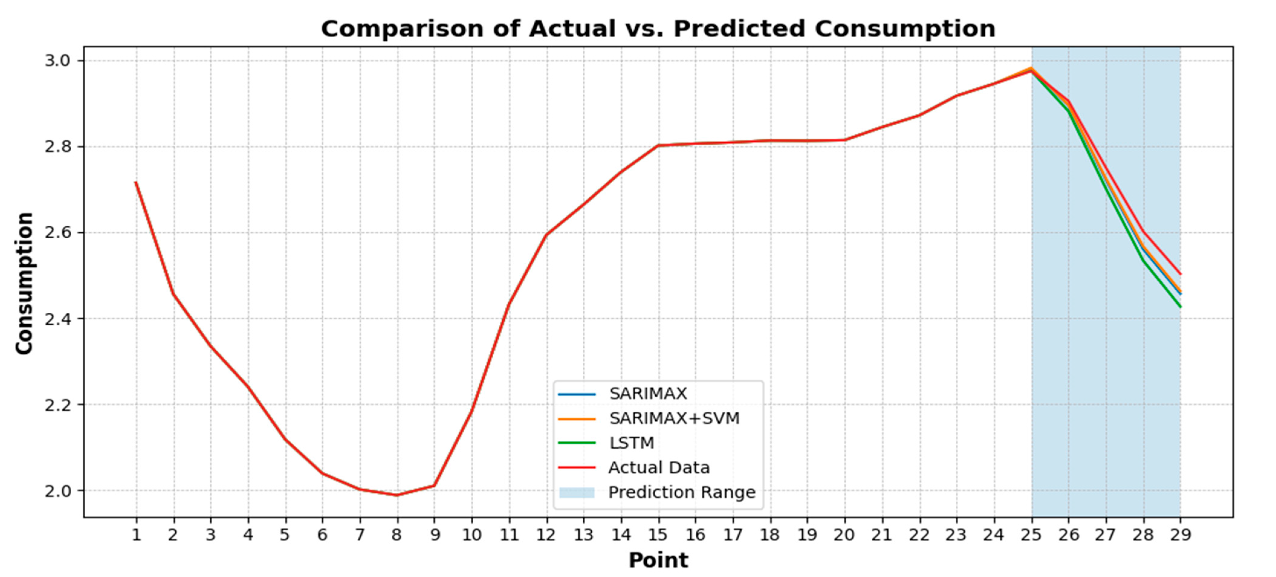
| Points | Actual Data | SVM | SARIMAX | SARIMAX-SVM | LSTM | DT | LR |
|---|---|---|---|---|---|---|---|
| 1 | 2.7142 | 2.6015 | 2.6639 | 2.6643 | 2.5890 | 2.5957 | 2.6134 |
| 2 | 2.4560 | 2.3966 | 2.4690 | 2.4344 | 2.5842 | 2.4083 | 2.3944 |
| 3 | 2.3348 | 2.3481 | 2.4151 | 2.3484 | 2.4777 | 2.3426 | 2.3371 |
| 4 | 2.2407 | 2.3904 | 2.3956 | 2.2992 | 2.2989 | 2.5218 | 2.3509 |
| 5 | 2.1184 | 2.3425 | 2.3332 | 2.2162 | 2.1163 | 2.5564 | 2.3206 |
| 6 | 2.0390 | 2.3999 | 2.2708 | 2.1503 | 2.0707 | 2.2839 | 2.3288 |
| 7 | 2.0019 | 2.3812 | 2.2343 | 2.1183 | 2.1638 | 2.2340 | 2.3469 |
| 8 | 1.9885 | 2.2186 | 2.2119 | 2.1052 | 2.2506 | 2.2557 | 2.2873 |
| 9 | 2.0104 | 2.2542 | 2.1978 | 2.1095 | 2.2660 | 2.1821 | 2.2571 |
| 10 | 2.1826 | 2.3480 | 2.3251 | 2.2581 | 2.3503 | 2.2845 | 2.3648 |
| 11 | 2.4312 | 2.5364 | 2.5075 | 2.4677 | 2.4726 | 2.3892 | 2.5374 |
| 12 | 2.5925 | 2.5118 | 2.6105 | 2.5944 | 2.5176 | 2.5190 | 2.5796 |
| 13 | 2.6633 | 2.5209 | 2.6243 | 2.6300 | 2.5002 | 2.4803 | 2.5489 |
| 14 | 2.7386 | 2.5162 | 2.6607 | 2.6812 | 2.5322 | 2.4634 | 2.5464 |
| 15 | 2.8005 | 2.5569 | 2.7059 | 2.7328 | 2.5907 | 2.6012 | 2.5706 |
| 16 | 2.8049 | 2.5523 | 2.7000 | 2.7302 | 2.6029 | 2.6616 | 2.5567 |
| 17 | 2.8078 | 2.6193 | 2.7314 | 2.7517 | 2.6543 | 2.7387 | 2.6047 |
| 18 | 2.8121 | 2.8028 | 2.7914 | 2.7927 | 2.7578 | 2.9074 | 2.7348 |
| 19 | 2.8116 | 3.0136 | 2.8453 | 2.8277 | 2.9006 | 2.9053 | 2.9066 |
| 20 | 2.8131 | 2.8910 | 2.8782 | 2.8489 | 2.9880 | 2.7959 | 2.9388 |
| 21 | 2.8432 | 2.8151 | 2.9128 | 2.8805 | 2.9828 | 2.7885 | 2.8989 |
| 22 | 2.8704 | 2.7953 | 2.9080 | 2.8846 | 2.8775 | 2.7140 | 2.8317 |
| 23 | 2.9160 | 2.7785 | 2.9365 | 2.9175 | 2.8068 | 2.7983 | 2.8109 |
| 24 | 2.9439 | 2.7573 | 2.8954 | 2.9234 | 2.8334 | 2.7480 | 2.7514 |
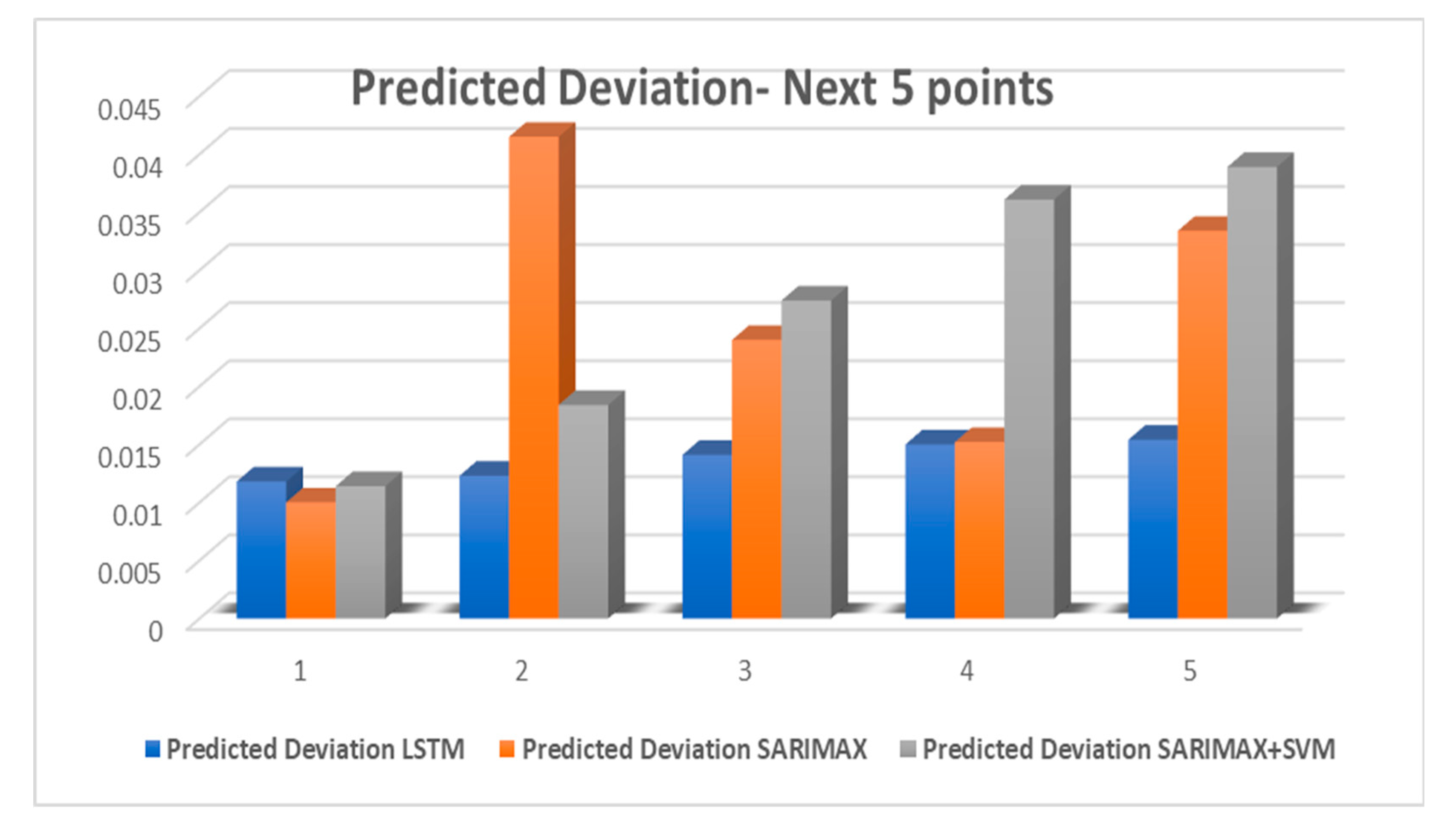
| Predicted Consumption | Predicted Deviation | ||||
|---|---|---|---|---|---|
| LSTM | SARIMAX | SARIMAX + SVM | LSTM | SARIMAX | SARIMAX + SVM |
| 2.9623 | 2.9698 | 2.9696 | 0.0118 | 0.01 | 0.0114 |
| 2.868 | 2.852 | 2.8763 | 0.0123 | 0.0415 | 0.0184 |
| 2.6871 | 2.6976 | 2.6977 | 0.0141 | 0.024 | 0.0274 |
| 2.5187 | 2.5452 | 2.5309 | 0.0150 | 0.0152 | 0.0361 |
| 2.4111 | 2.4233 | 2.4239 | 0.0154 | 0.0334 | 0.0389 |
| Actual | Predicted Consumption by Proposed Methods | Predicted Consumption Without DC | |||||||
|---|---|---|---|---|---|---|---|---|---|
| Real Data | LSTM-DC | SARIMAX-DC | SARIMAX-SVM-DC | LSTM | SARIMAX | SARIMAX SVM | SVM | LR | DT |
| 2.9734 | 2.9741 | 2.9798 | 2.981 | 2.9623 | 2.9698 | 2.9696 | 2.9108 | 2.9201 | 2.9267 |
| 2.9042 | 2.8803 | 2.8935 | 2.8947 | 2.868 | 2.852 | 2.8763 | 2.8002 | 2.8065 | 2.7971 |
| 2.7497 | 2.7012 | 2.7216 | 2.7251 | 2.6871 | 2.6976 | 2.6977 | 2.5907 | 2.5951 | 2.6522 |
| 2.6016 | 2.5337 | 2.5604 | 2.567 | 2.5187 | 2.5452 | 2.5309 | 2.4679 | 2.4688 | 2.5314 |
| 2.5026 | 2.4265 | 2.4567 | 2.4628 | 2.4111 | 2.4233 | 2.4239 | 2.3556 | 2.3538 | 2.4221 |
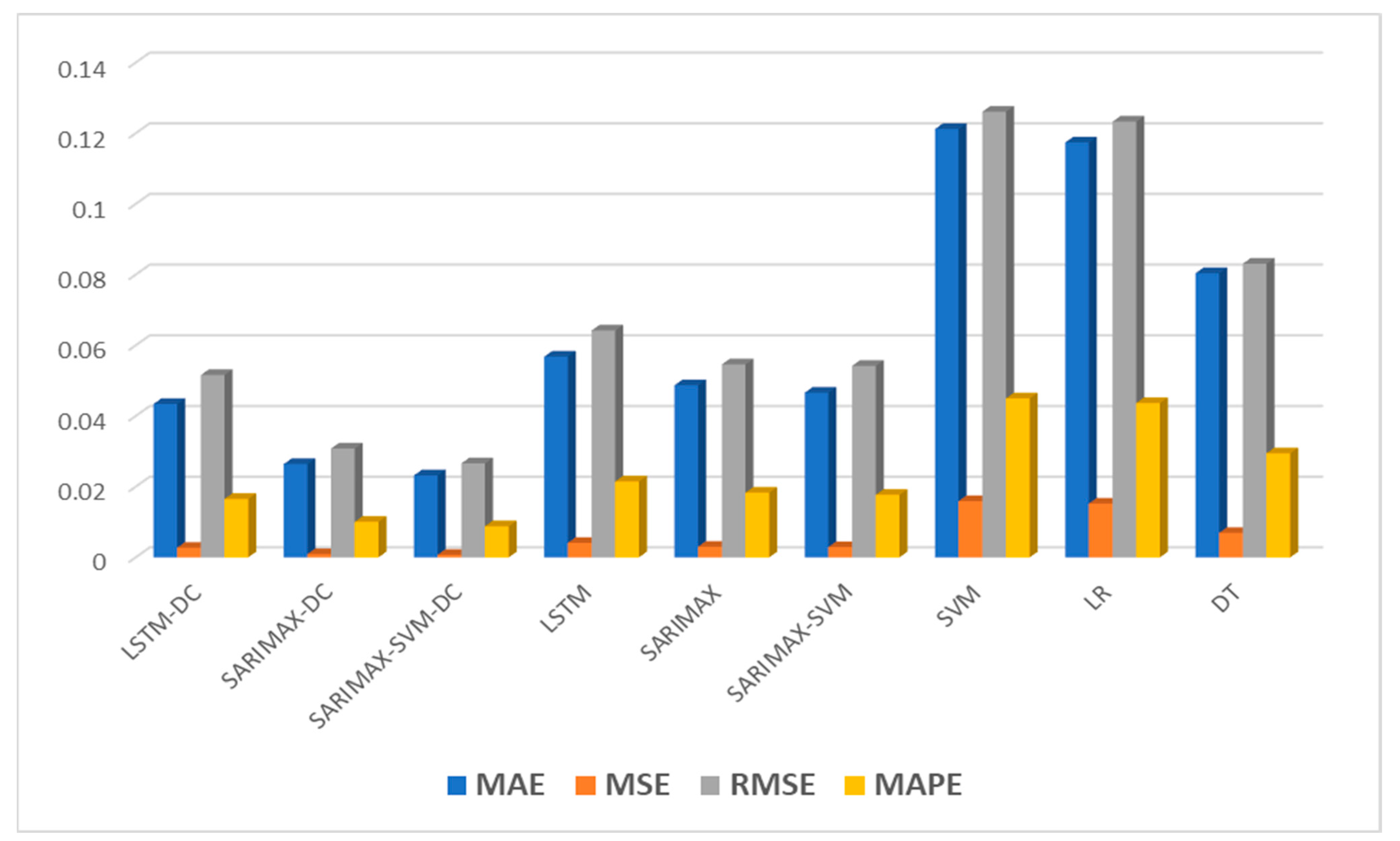
| Metric | CM-LSTM-DC | CM-SARIMAX-DC | CM-SARIMAX-SVM-DC |
|---|---|---|---|
| MAE | 0.0434 | 0.0264 | 0.0232 |
| MSE | 0.0027 | 0.0009 | 0.0007 |
| RMSE | 0.0516 | 0.0308 | 0.0266 |
| MAPE | 1.65% | 1.00% | 0.88% |
Disclaimer/Publisher’s Note: The statements, opinions and data contained in all publications are solely those of the individual author(s) and contributor(s) and not of MDPI and/or the editor(s). MDPI and/or the editor(s) disclaim responsibility for any injury to people or property resulting from any ideas, methods, instructions or products referred to in the content. |
© 2025 by the authors. Licensee MDPI, Basel, Switzerland. This article is an open access article distributed under the terms and conditions of the Creative Commons Attribution (CC BY) license (https://creativecommons.org/licenses/by/4.0/).
Share and Cite
Hassanpouri Baesmat, K.; Farrokhi, Z.; Chmaj, G.; Regentova, E.E. Parallel Multi-Model Energy Demand Forecasting with Cloud Redundancy: Leveraging Trend Correction, Feature Selection, and Machine Learning. Forecasting 2025, 7, 25. https://doi.org/10.3390/forecast7020025
Hassanpouri Baesmat K, Farrokhi Z, Chmaj G, Regentova EE. Parallel Multi-Model Energy Demand Forecasting with Cloud Redundancy: Leveraging Trend Correction, Feature Selection, and Machine Learning. Forecasting. 2025; 7(2):25. https://doi.org/10.3390/forecast7020025
Chicago/Turabian StyleHassanpouri Baesmat, Kamran, Zeinab Farrokhi, Grzegorz Chmaj, and Emma E. Regentova. 2025. "Parallel Multi-Model Energy Demand Forecasting with Cloud Redundancy: Leveraging Trend Correction, Feature Selection, and Machine Learning" Forecasting 7, no. 2: 25. https://doi.org/10.3390/forecast7020025
APA StyleHassanpouri Baesmat, K., Farrokhi, Z., Chmaj, G., & Regentova, E. E. (2025). Parallel Multi-Model Energy Demand Forecasting with Cloud Redundancy: Leveraging Trend Correction, Feature Selection, and Machine Learning. Forecasting, 7(2), 25. https://doi.org/10.3390/forecast7020025