
Mode Decomposition Bi-Directional Long Short-Term Memory (BiLSTM) Attention Mechanism and Transformer (AMT) Model for Ozone (O3) Prediction in Johannesburg, South Africa


Abstract
1. Introduction
2. Materials and Methods
2.1. Study Area
2.2. Model Development
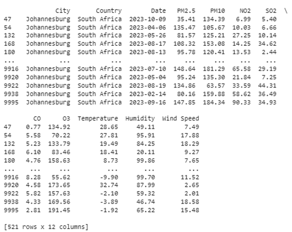
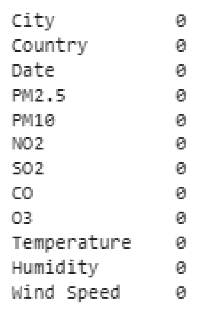
2.2.1. Pre-Processing Layer
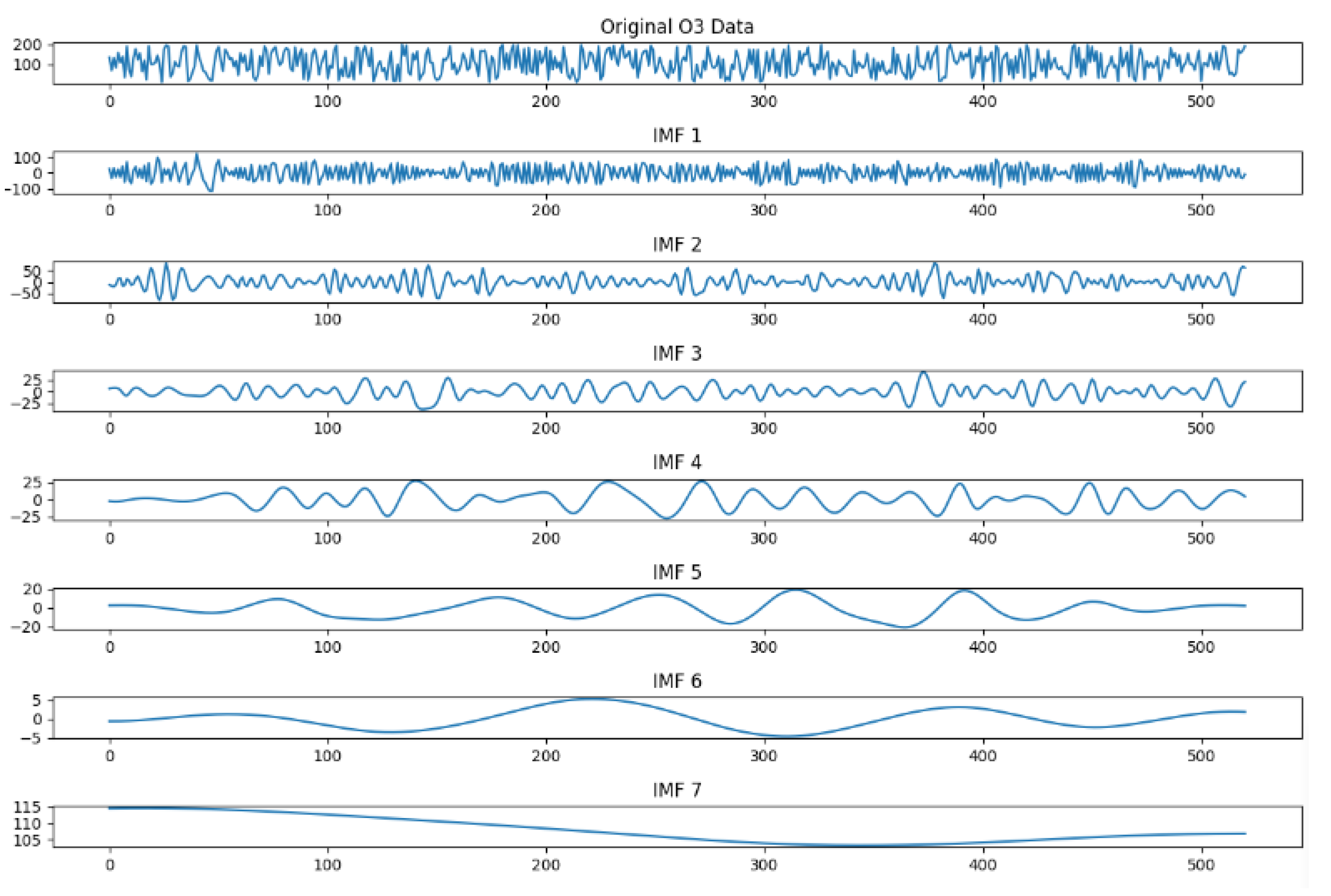
2.2.2. Mode Decomposition Approach
2.2.3. BiLSTM Layer
2.2.4. Attention Mechanism Transformer Layer
2.2.5. Model Evaluation
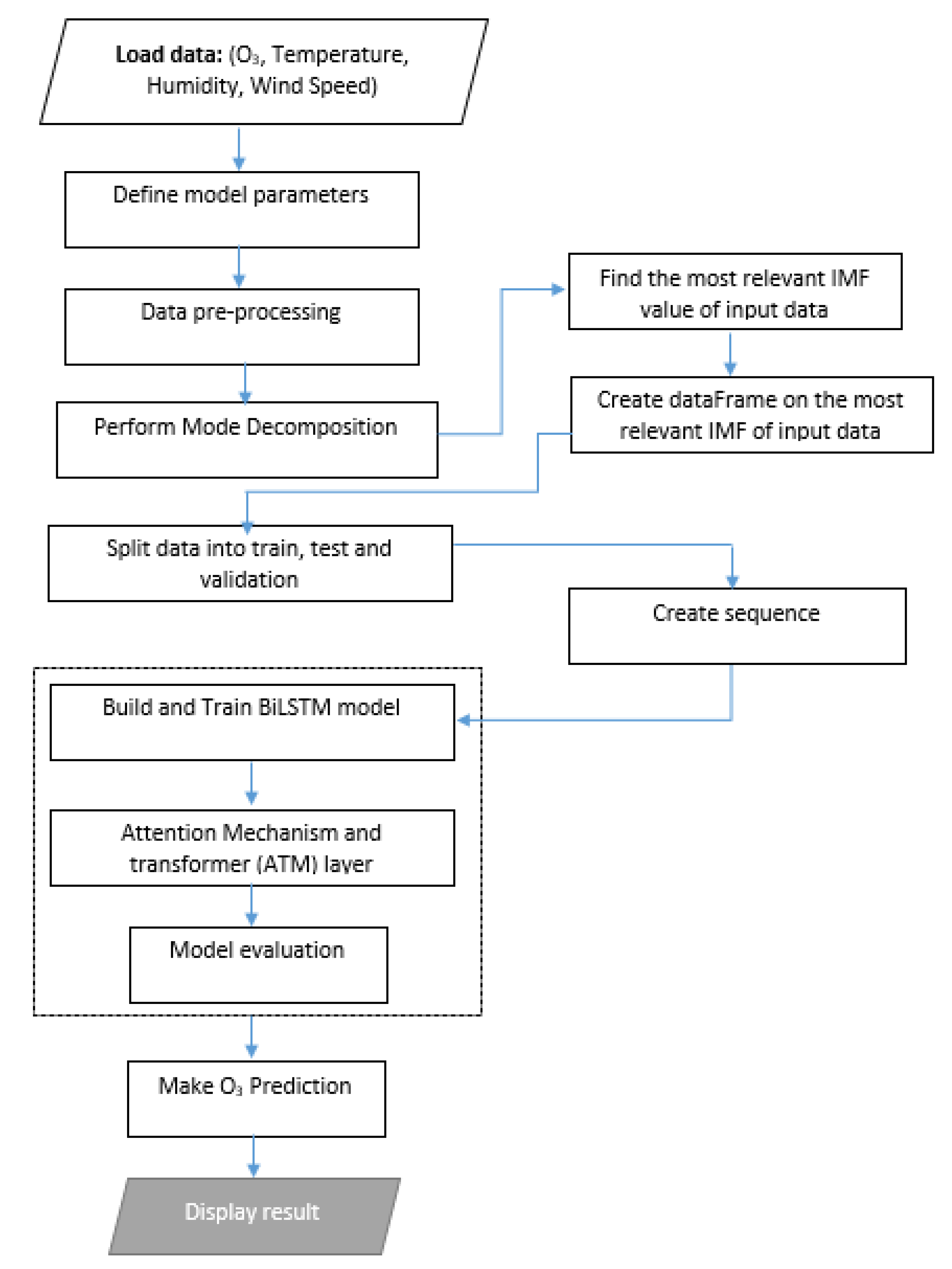
2.3. Flowchart of the Proposed Model
2.4. Model Description and Parameters
3. Results
4. Discussions
5. Conclusions and Future Directions
Author Contributions
Funding
Data Availability Statement
Conflicts of Interest
Appendix A. Implementation Algorithm
| Algorithm A1: Data Pre-Processing Layer |
| Input: Load original unprocessed data in CSV file format Output: Clean data for Johannesburg in CSV file format |
| Process 1.1: Import libraries Process 1.2: Load CSV file Process 1.3: Extract country and city Process 1.4: Rename the columns Process 1.5: Re-engineer timestamp into day, hour, and year Process 1.6: Remove empty entries Process 1.7: Print (Output the clean data) |
| Algorithm A2: Mode Decomposition Layer |
| Input: Load the clean_data.csv Output: Most relevant IMF |
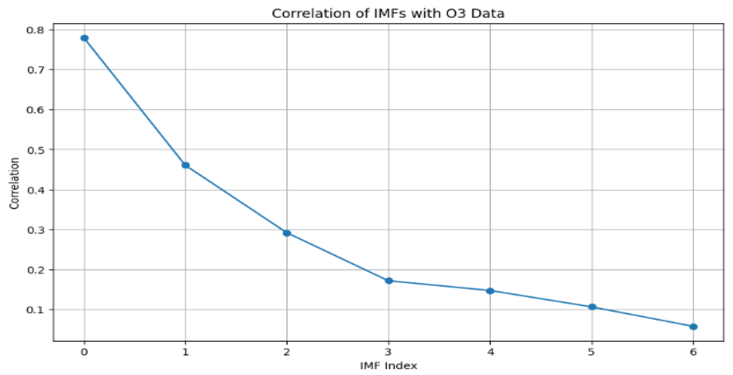
| Process 2.1: Load data (e.g., O3 concentration) Process 2.2: Perform EEMD Process 2.3: Calculate the correlation between IMF and original data Process 2.4: Find the IMF with the highest correlation Process 2.5: Output the most relevant IMF and correlation with O3 |
| Algorithm A3: Analysis of IMFs |
| Input: Most relevant IMF Output: Statistical properties of IMF |
| Process 3.1: Analyze the frequency of IMF Process 3.2: Perform statistical analysis of each IMF Process 3.3: Calculate the PSD Process 3.4: Find the peaks in PDS Process 3.5: Print frequencies Process 3.6: Plot the frequencies and PDS with peak marks Process 3.7: Output the statistical value of the IMF |
| Algorithm A4: BiLSTM Layer for Training |
| Input: Most relevant IMF Output: Model for prediction of O3 |
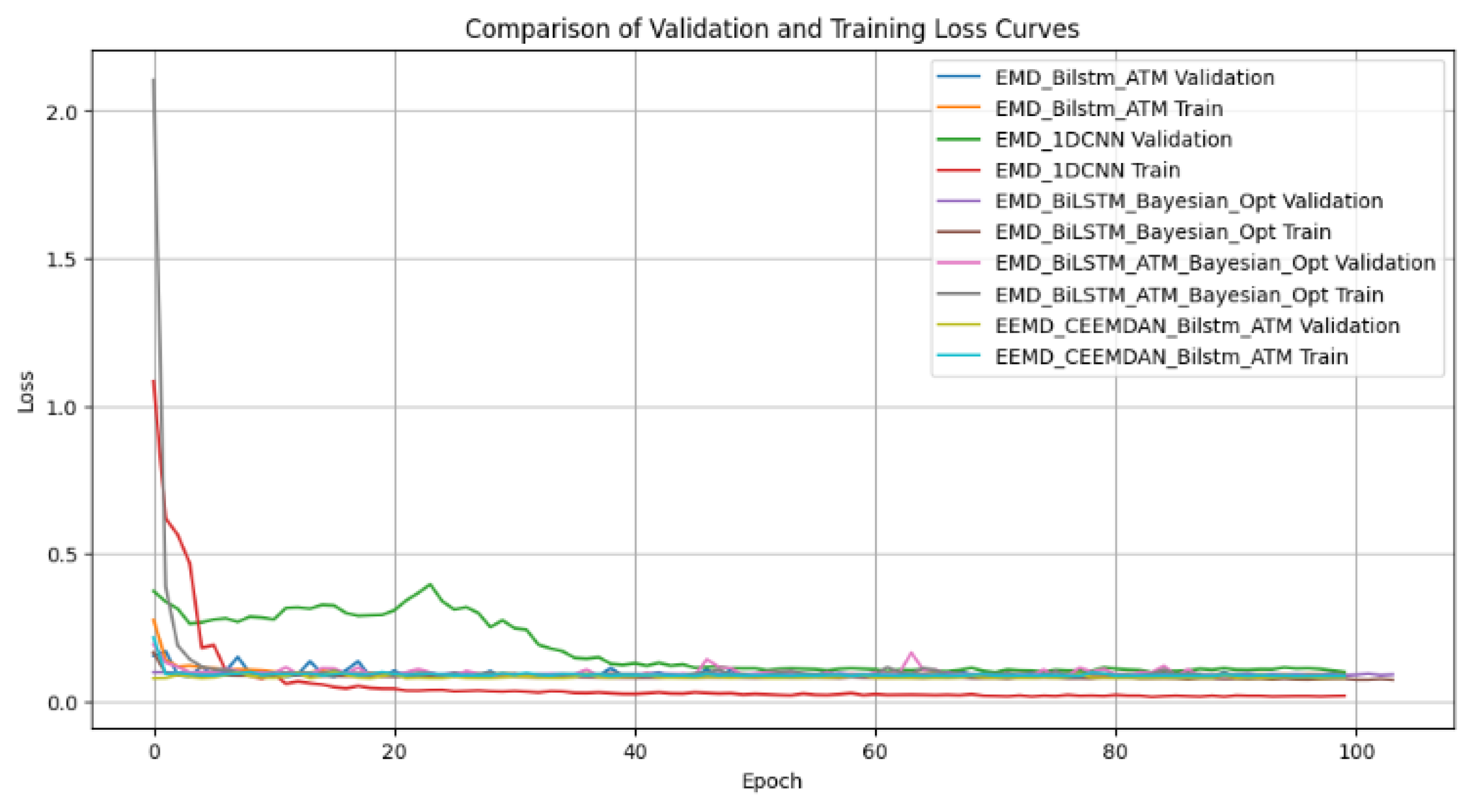
| Process 4.1: Normalize and reshape data Process 4.2: Split data into test, training, and validation Process 4.3: Create BiLSTM layer with input sequence as the most relevant IMF Process 4.4: Hyper-parameter settings on BiLSTM Process 4.5: Create an Attention mechanism layer Process 4.6: Create a transformer layer with dropout and layer normalization Process 4.7: Dense layer final output Process 4.8: Create the hybrid model for training Process 4.9: Evaluate the model Process 4.10: Output evaluation performance Process 4.11: Inverse transform the prediction to the original scale Process 4.12: Output the graph on training, test, and validation loss |
Appendix B. Dataset
References
- Samad, A.; Garuda, S.; Vogt, U.; Yang, B. Air pollution prediction using machine learning techniques—An approach to replace existing monitoring stations with virtual monitoring stations. Atmos. Environ. 2023, 310, 119987. [Google Scholar] [CrossRef]
- Pan, Q.; Harrou, F.; Sun, Y. A comparison of machine learning methods for ozone pollution prediction. J. Big Data 2023, 10, 63. [Google Scholar] [CrossRef]
- Abdullah, S.; Nasir, N.H.A.; Ismail, M.; Ahmed, A.N.; Jarkoni, M.N.K. Development of Ozone Prediction Model in Urban Area. Int. J. Innov. Technol. Explor. Eng. 2019, 8, 2263–2267. [Google Scholar]
- Igamba, J. Air Pollution in South Africa: The Silent Killer That Demands Urgent Action. 2023. Available online: https://www.greenpeace.org/africa/en/blog/54600/air-pollution-in-south-africa-the-silent-killer-that-demands-urgent-action/ (accessed on 7 September 2024).
- Morakinyo, O.M.; Mukhola, M.S.; Mokgobu, M.I. Ambient Gaseous Pollutants in an Urban Area in South Africa: Levels and Potential Human Health Risk. Atmosphere 2020, 11, 751. [Google Scholar] [CrossRef]
- Sharma, S.; Joshi, J.; Kataria, S.; Verma, S.K.; Chatterjee, S.; Jain, M.; Brestic, M. Chapter 27—Regulation of the Calvin cycle under abiotic stresses: An overview. In Plant Life Under Changing Environment; Tripathi, D.K., Chauhan, D.K., Sharma, S., Prasad, S.P., Dubey, N.K., Ramawat, K., Eds.; Academic Press: Cambridge, MA, USA, 2020; pp. 681–717. [Google Scholar]
- Agency, U.S.E.P. Ozone and Your Patients’ Health. 2024. Available online: https://www.epa.gov/ozone-pollution-and-your-patients-health (accessed on 20 September 2024).
- Wu, C.-L.; He, H.-D.; Song, R.-F.; Zhu, X.-H.; Peng, Z.-R.; Fu, Q.-Y.; Pan, J. A hybrid deep learning model for regional O3 and NO2 concentrations prediction based on spatiotemporal dependencies in air quality monitoring network. Environ. Pollut. 2023, 320, 121075. [Google Scholar] [CrossRef] [PubMed]
- Yafouz, A.; AlDahoul, N.; Birima, A.H.; Ahmed, A.N.; Sherif, M.; Sefelnasr, A.; Allawi, M.F.; Elshafie, A. Comprehensive comparison of various machine learning algorithms for short-term ozone concentration prediction. Alex. Eng. J. 2022, 61, 4607–4622. [Google Scholar] [CrossRef]
- Yang, J.; Zhao, Y. Performance and application of air quality models on ozone simulation in China—A review. Atmospheric Environ. 2023, 293, 119446. [Google Scholar] [CrossRef]
- Wang, S.; Sun, Y.; Gu, H.; Cao, X.; Shi, Y.; He, Y. A deep learning model integrating a wind direction-based dynamic graph network for ozone prediction. Sci. Total. Environ. 2024, 946, 174229. [Google Scholar] [CrossRef] [PubMed]
- Donzelli, G.; Suarez-Varela, M.M. Tropospheric Ozone: A Critical Review of the Literature on Emissions, Exposure, and Health Effects. Atmosphere 2024, 15, 779. [Google Scholar] [CrossRef]
- Xiao, H. A Hybrid Model Integrating LSTM with GARCH Family Models for the Ozone Concentration Prediction. In Proceedings of the 2023 3rd International Conference on Computer Science, Electronic Information Engineering and Intelligent Control Technology (CEI), Wuhan, China, 15–17 December 2013; pp. 1–6. [Google Scholar]
- Yar, A.; Henna, S.; McAfee, M.; Gharbia, S.S. Air Pollution Monitoring Using Online Recurrent Extreme Learning Machine. In Proceedings of the 2023 31st Irish Conference on Artificial Intelligence and Cognitive Science (AICS), Letterkenny, Ireland, 7–8 December 2023; pp. 1–6. [Google Scholar]
- Cao, J.; Bhatti, U.A.; Feng, S.; Huang, M.; Hasnain, A. Air Quality Index Predictions with a Hybrid Forecasting Model: Combining Series Decomposition and Deep Learning Techniques. In Proceedings of the 2023 IEEE 6th International Conference on Pattern Recognition and Artificial Intelligence (PRAI), Haikou, China, 18–20 August 2023. [Google Scholar]
- Du, X.; Yuan, Z.; Huang, D.; Ma, W.; Yang, J.; Mo, J. Importance of secondary decomposition in the accurate prediction of daily-scale ozone pollution by machine learning. Sci. Total. Environ. 2023, 904, 166963. [Google Scholar] [CrossRef] [PubMed]
- Pei, Y.; Huang, C.-J.; Shen, Y.; Ma, Y. An Ensemble Model with Adaptive Variational Mode Decomposition and Multivariate Temporal Graph Neural Network for PM2.5 Concentration Forecasting. Sustainability 2022, 14, 13191. [Google Scholar] [CrossRef]
- Sun, W.; Huang, C. A hybrid air pollutant concentration prediction model combining secondary decomposition and sequence reconstruction. Environ. Pollut. 2020, 266, 115216. [Google Scholar] [CrossRef] [PubMed]
- Wang, X.; Zhang, S.; Chen, Y.; He, L.; Ren, Y.; Zhang, Z.; Li, J.; Zhang, S. Air quality forecasting using a spatiotemporal hybrid deep learning model based on VMD–GAT–BiLSTM. Sci. Rep. 2024, 14, 17841. [Google Scholar] [CrossRef] [PubMed]
- Borduas-Dedekind, N.; Naidoo, M.; Zhu, B.; Geddes, J.; Garland, R.M. Tropospheric ozone (O3) pollution in Johannesburg, South Africa: Exceedances, diurnal cycles, seasonality, Ox chemistry and O3 production rates. Clean Air J. 2023, 33, 1–16. [Google Scholar] [CrossRef]
- Matandirotya, N.R.; Dangare, T.; Matandirotya, E.; Mahed, G. Characterisation of ambient air quality over two urban sites on the South African Highveld. Sci. Afr. 2023, 19, e01530. [Google Scholar] [CrossRef]
- Wattal, K.; Singh, S.K. Multivariate Air Pollution Levels Forecasting. In Proceedings of the 2021 2nd International Conference on Advances in Computing, Communication, Embedded and Secure Systems (ACCESS), Ernakulam, India, 2–4 September 2021. [Google Scholar]
- Jiang, X.; Wei, P.; Luo, Y.; Li, Y. Air pollutant concentration prediction based on a CEEMDAN-FE-BiLSTM model. Atmosphere 2021, 12, 1452. [Google Scholar] [CrossRef]
- Chen, X.; Li, Y.; Xu, X.; Shao, M. A Novel Interpretable Deep Learning Model for Ozone Prediction. Appl. Sci. 2023, 13, 11799. [Google Scholar] [CrossRef]
- Zang, Z.; Guo, Y.; Jiang, Y.; Zuo, C.; Li, D.; Shi, W.; Yan, X. Tree-based ensemble deep learning model for spatiotemporal surface ozone (O3) prediction and interpretation. Int. J. Appl. Earth Obs. Geoinf. 2021, 103, 102516. [Google Scholar] [CrossRef]
- Barnes, P.W.; Williamson, C.E.; Lucas, R.M.; Robinson, S.A.; Madronich, S.; Paul, N.D.; Bornman, J.F.; Bais, A.F.; Sulzberger, B.; Wilson, S.R.; et al. Ozone depletion, ultraviolet radiation, climate change and prospects for a sustainable future. Nat. Sustain. 2019, 2, 569–579. [Google Scholar] [CrossRef]

| Hyper-Parameter | Value |
|---|---|
| Batch size | 32 |
| Maximum epoch | 100 |
| Dropout | 0.1 |
| Epoch | 100 |
| Learning rate | 0.01 |
| Units | 50 |
| Features | Min | Max | Mean | Variance |
|---|---|---|---|---|
| PM2.5 | 5.02 | 149.78 | 77.6660 | 1663.56 |
| PM10 | 10.00 | 199.99 | 105.1351 | 3162.87 |
| NO2 | 5.83 | 99.98 | 53.1469 | 752.70 |
| SO2 | 1.02 | 49.93 | 24.6742 | 207.35 |
| CO | 0.10 | 9.97 | 5.09339 | 7.55 |
| O3 | 10.05 | 199.76 | 106.1828 | 3095.26 |
| Temperature | −9.93 | 39.97 | 14.45266 | 206.79 |
| Relative Humidity | 10.05 | 99.86 | 55.44952 | 647.58 |
| Wind Speed | 0.50 | 20.00 | 10.08606 | 31.25 |
| IMF | Mean | Standard Deviation | Skewness | Kurtosis |
|---|---|---|---|---|
| 1 | −0.42202 | 44.9020 | −0.02123 | −1.0677 |
| 2 | −0.1517 | 27.5651 | −0.00772 | 0.26913 |
| 3 | −0.50037 | 13.6808 | −0.09326 | 0.2250 |
| 4 | 0.35778 | 12.0271 | −0.00269 | −0.4866 |
| 5 | −1.0607 | 9.0833 | 0.0859 | −0.59361 |
| 6 | 0.02320 | 2.5492 | 0.14982 | −0.7002 |
| 7 | 107.9368 | 3.85897 | 0.49060 | −1.1875 |
| IMF Index | IMF | Correlation of Each IMF with O3 |
|---|---|---|
| 0 | IMF1 | 0.7797 |
| 1 | IMF2 | 0.4603 |
| 2 | IMF3 | 0.2915 |
| 3 | IMF4 | 0.1715 |
| 4 | IMF5 | 0.1471 |
| 5 | IMF6 | 0.1061 |
| 6 | IMF7 | 0.0575 |
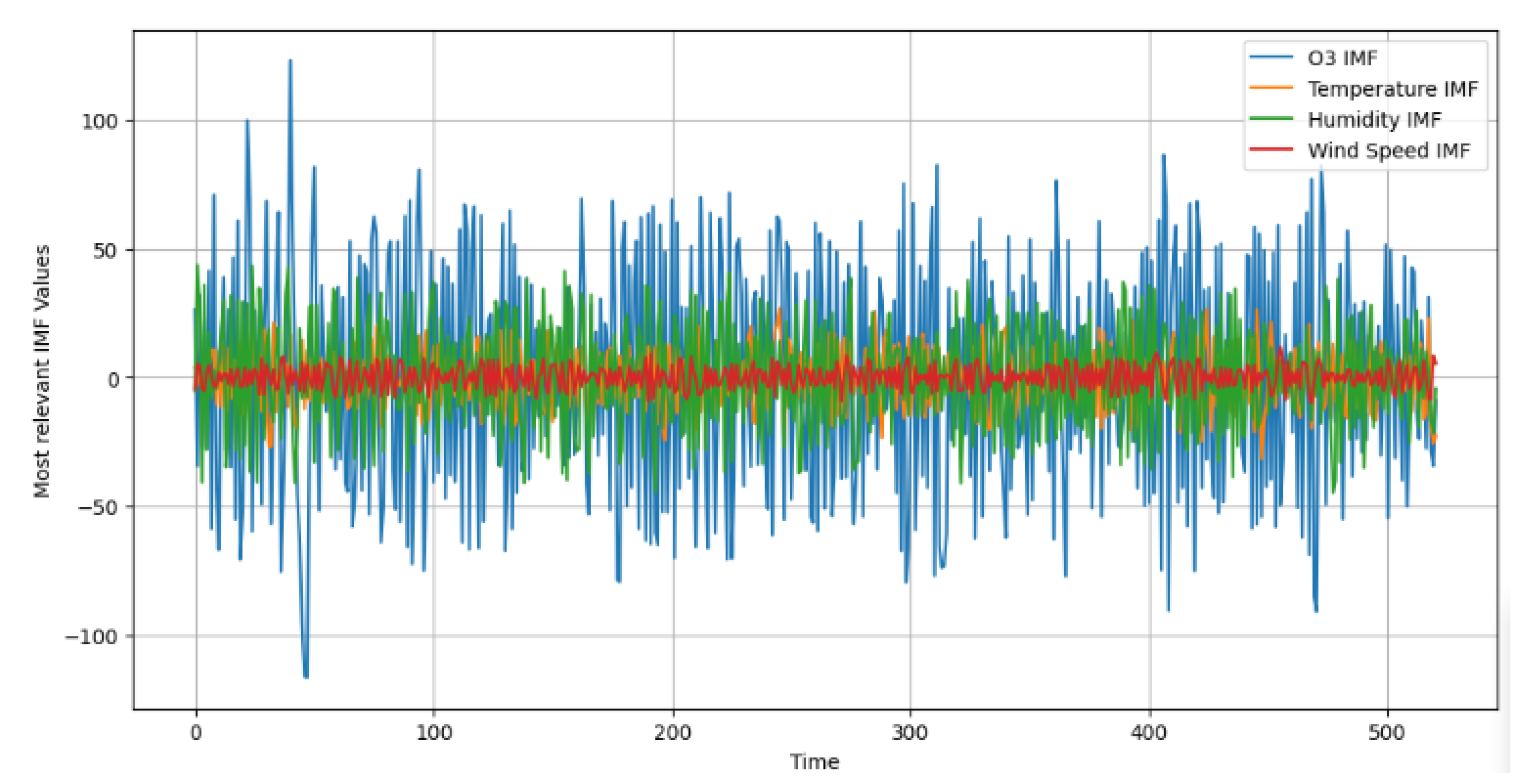
| IMF Features | Correlation |
|---|---|
| Temperature IMF | 0.8206 |
| Humidity IMF | 0.8632 |
| Wind speed IMF | 0.8025 |
| Models | Validation Loss | Test Loss |
|---|---|---|
| EMD-BiLSTM-AMT | 0.088 | 0.065 |
| EMD-1DCNN | 0.099 | 0.081 |
| EMD-BiLSTM-Bayesian Opt. | 0.090 | 0.068 |
| EMD-BiLSTM-AMT-Bayesian Opt. | 0.103 | 0.083 |
| EEMD-CEEMDAN-BiLSTM-AMT | 6.32 × 10⁻⁶ | 6.35 × 10⁻⁶ |
| Models | MSE | RMSE | MAE |
|---|---|---|---|
| EMD-BiLSTM-AMT | 0.065 | 0.254 | 0.211 |
| EMD-1DCNN | 13,277.24 | 115.22 | 102.915 |
| EMD-BiLSTM-Bayesian Opt. | 0.068 | 0.239 | 0.194 |
| EMD-BiLSTM-AMT-Bayesian Opt. | 3001.06 | 54.78 | 47.056 |
| EEMD-CEEMDAN-BiLSTM-AMT | 4.80 × 10⁻⁶ | 0.002 | 0.0019 |
| Temperature | Humidity | Wind Speed | O3 | |
|---|---|---|---|---|
| Temperature | 1.000000 | −0.067947 | −0.062734 | −0.001001 |
| Humidity | −0.067947 | 1.000000 | −0.040013 | 0.103426 |
| Wind Speed | −0.062734 | −0.040013 | 1.000000 | −0.050442 |
| O3 | −0.001001 | 0.103426 | −0.050442 | 1.000000 |
| O3 IMF | Temperature IMF | Humidity IMF | Wind Speed IMF | |
|---|---|---|---|---|
| O3 IMF | 1.0000 | 0.0226 | 0.0854 | −0.0648 |
| Temperature IMF | 0.0224 | 1.0000 | −0.0153 | −0.0942 |
| Humidity IMF | 0.0854 | −0.0153 | 1.0000 | −0.0534 |
| Wind Speed IMF | −0.0648 | −0.0942 | −0.0534 | 1.0000 |
Disclaimer/Publisher’s Note: The statements, opinions and data contained in all publications are solely those of the individual author(s) and contributor(s) and not of MDPI and/or the editor(s). MDPI and/or the editor(s) disclaim responsibility for any injury to people or property resulting from any ideas, methods, instructions or products referred to in the content. |
© 2025 by the authors. Licensee MDPI, Basel, Switzerland. This article is an open access article distributed under the terms and conditions of the Creative Commons Attribution (CC BY) license (https://creativecommons.org/licenses/by/4.0/).
Share and Cite
Agbehadji, I.E.; Obagbuwa, I.C. Mode Decomposition Bi-Directional Long Short-Term Memory (BiLSTM) Attention Mechanism and Transformer (AMT) Model for Ozone (O3) Prediction in Johannesburg, South Africa. Forecasting 2025, 7, 15. https://doi.org/10.3390/forecast7020015
Agbehadji IE, Obagbuwa IC. Mode Decomposition Bi-Directional Long Short-Term Memory (BiLSTM) Attention Mechanism and Transformer (AMT) Model for Ozone (O3) Prediction in Johannesburg, South Africa. Forecasting. 2025; 7(2):15. https://doi.org/10.3390/forecast7020015
Chicago/Turabian StyleAgbehadji, Israel Edem, and Ibidun Christiana Obagbuwa. 2025. "Mode Decomposition Bi-Directional Long Short-Term Memory (BiLSTM) Attention Mechanism and Transformer (AMT) Model for Ozone (O3) Prediction in Johannesburg, South Africa" Forecasting 7, no. 2: 15. https://doi.org/10.3390/forecast7020015
APA StyleAgbehadji, I. E., & Obagbuwa, I. C. (2025). Mode Decomposition Bi-Directional Long Short-Term Memory (BiLSTM) Attention Mechanism and Transformer (AMT) Model for Ozone (O3) Prediction in Johannesburg, South Africa. Forecasting, 7(2), 15. https://doi.org/10.3390/forecast7020015