Testing for Bias in Forecasts for Independent Multinomial Outcomes

Abstract

This paper deals with a test on forecast bias in predicting independent multinomial outcomes where the predictions are probabilities. The new Likelihood Ratio (and Wald) test extends the familiar Mincer Zarnowitz regression to a multinomial logit model instead of a linear regression. The test is evaluated using various simulation experiments, which indicate that the size and power properties are good, even for small sample sizes, in the sense that the size is close to the used 5% level, and the power quickly reaches 1. We implement the test in an empirical setting on brand choice by individual households.

1. Introduction and Motivation

This paper addresses the evaluation of predictions from multinomial models. Such an evaluation is relevant the assess the quality of these models, which are often applied in consumer choice analysis, marketing research, transportation research and more.

There are various tests for the accuracy of multinomial models. There are tests for the goodness of fit, like the Pearson ${\chi }^2$ test and the Brier score. Also, there are tests based on the prediction realization table and on cross-entropy loss (see [1] for a recent survey.). These tests all concern a measure of the fit. In contrast, in this paper, we propose a Likelihood Ratio (and Wald) test on forecast bias in predicting $J$ independent multinomial outcomes, where the outcomes can be $1,2,\dots ,J$ and where the predictions are probabilities. Such multinomial outcomes are frequently observed in transportation mode choice and brand choice. The probabilities are given from the outset and can be based on an econometric model, like a multinomial probit or multinomial logit model, and they can also be created by experts, who do not necessarily rely on an econometric model. This is an advantage of our simple test.

A useful tool to test for bias forecasts for continuous variables is the so-called Mincer–Zarnowitz regression, by [2]. If realizations $y_i$ and forecasts ${\widehat{y}}_i$ are continuous variables, and these can be cross sectional data or time series data, where the forecast sample is $i=1,2,\dots ,N$, then the auxiliary regression

$$y_i=\alpha +\beta {\widehat{y}}_i+{\epsilon }_i,$$

where ${\epsilon }_i$ is a mean zero uncorrelated error process, can be used to test bias. The parameters can be estimated using Ordinary Least Squares (OLS). The Wald type test of interest concerns the null hypothesis that $\alpha =0$ and $\beta =1$, jointly. Under the null hypothesis, there is no forecast bias.

In this paper, we propose a similar test but now for independent multinomial outcomes, which in a sense extends on the test for binomial outcomes in [3]. There are realizations that can be either $1,2,\dots ,\mathrm{o}\mathrm{r} J$, and the predictions are estimated probabilities of each of the $J$ outcomes. The question now is whether these predictions based on the probabilities are unbiased or not.

The new test is similarly as easy as the Mincer Zarnowitz regression, where now a multinomial logit model is used instead of a linear regression. This article proceeds in Section 2 with the proposed test. In Section 3, the test is evaluated using various simulation experiments. Section 4 implements the test to an empirical setting on brand choice by individual households. Section 5 concludes the article.

2. The Main Idea

Suppose there is a multinomial model for $J$ discrete choices, made by $N$ individuals, and that this model generates fitted probabilities ${\widehat{p}}_{ij}$ for $j=1,2,\dots ,J$ and $i=1,2,\dots ,N$. Consider the estimated odds of the probability of choosing $j$ versus $k$, that is,

$${\displaystyle \frac{\mathrm{Pr}[Y_i=j]}{\mathrm{Pr}[Y_i=k]}}={\displaystyle \frac{{\widehat{p}}_{ij}}{{\widehat{p}}_{ik}}}={\displaystyle \frac{\exp \left(\ln {\widehat{p}}_{ij}\right)}{\exp (\ln {\widehat{p}}_{ik})}}$$

(1)

for all $j,k\in \{1,2,\dots ,J\}$. The estimated odds imply that

$$\mathrm{Pr}\left[Y_i=j\right]={\displaystyle \frac{\exp \left(\ln {\widehat{p}}_{ij}\right)}{{\sum }_{l=1}^J\exp \left(\ln {\widehat{p}}_{il}\right)}}$$

(2)

In case of a predictive bias, the odds ratios are incorrect.

To describe potential bias, we extend (1) by adding intercepts and a slope parameter (alternative to 1), which results in

$${\displaystyle \frac{\mathrm{Pr}[Y_i=j]}{\mathrm{Pr}[Y_i=k]}}={\displaystyle \frac{{\widehat{p}}_{ij}}{{\widehat{p}}_{ik}}}={\displaystyle \frac{\exp ({\alpha }_j+\beta \ln {\widehat{p}}_{ij})}{\exp ({\alpha }_l+\beta \ln {\widehat{p}}_{ik})}}$$

(3)

This implies that the choice probabilities in (2) can be written as

$$\mathrm{Pr}\left[Y_i=j\right]={\displaystyle \frac{\exp ({\alpha }_j+\beta \ln {\widehat{p}}_{ij})}{{\sum }_{l=1}^J\exp ({\alpha }_l+\beta \ln {\widehat{p}}_{il})}}$$

(4)

with the assumption that ${\alpha }_J=0$ for identification, where J can be any of the choices.

Under the joint null hypothesis

$${\alpha }_1={\alpha }_2=\cdots ={\alpha }_{J-1}=0\mathrm{and} \beta =1,$$

(5)

there is no bias in the estimated probabilities. We can use this result to test for bias in prediction probabilities by estimating the parameters in a multinomial logit model (MNL) in which the $Y$ variables are the out-of-sample realizations and the $\widehat{p}$ are the predicted probabilities from a statistical model if from the judgment of experts. We can use a Likelihood Ratio (LR) test or Wald test for the composite null hypothesis in (5).

The Likelihood Ratio test statistic is given by

$$LR=-2(l\left(0,\dots ,0,1\right)-l\left({\widehat{\alpha }}_1,\dots ,{\widehat{\alpha }}_{J-1},\widehat{\beta }\right))$$

(6)

where the log-likelihood function is given by

$$l\left({\alpha }_1,\dots ,{\alpha }_{J-1},\beta \right)$$

$$=\sum _{i=1}^N\left(\sum _{j=1}^J({\alpha }_j+\beta \ln {\widehat{p}}_{ij}\left)I\right[y_i=j]-\ln \left(\sum _{l=1}^J\mathrm{e}\mathrm{x}\mathrm{p}({\alpha }_l+\beta \ln {\widehat{p}}_{il})\right)\right)$$

(7)

and where $\left({\widehat{\alpha }}_1,\dots ,{\widehat{\alpha }}_{J-1},\widehat{\beta }\right)$ concern the unrestricted Maximum Likelihood estimates.

Let $\theta =({\alpha }_1,\dots ,{\alpha }_{J-1},\beta {)}^{\prime }$. The Wald test statistic is given by

$$W=\left({\widehat{\alpha }}_1,\dots ,{\widehat{\alpha }}_{J-1},\widehat{\beta }-1\right)V{\left(\widehat{\theta }\right)}^{-1}({\widehat{\alpha }}_1,\dots ,{\widehat{\alpha }}_{J-1},\widehat{\beta }-1{)}^{\prime }$$

(8)

where $V\left(\widehat{\theta }\right)$ denotes the covariance matrix of the Maximum Likelihood estimator

$$V\left(\theta \right)=-{\left({\displaystyle \frac{\partial l\left(\theta \right)}{\partial \theta \partial {\theta }^{\prime }}}\right)}^{-1}$$

(9)

evaluated in the Maximum Likelihood estimates $\widehat{\theta }={\left({\widehat{\alpha }}_1,\dots ,{\widehat{\alpha }}_{J-1},\widehat{\beta }\right)}^{\prime }$.

We can also implement partial tests to examine the absence of relative bias, for example by considering the null hypothesis ${\alpha }_1={\alpha }_2=\cdots ={\alpha }_{J-1}=0$. As we consider a joint test for zero restrictions on all α parameters, the proposed test statistic will be independent of the chosen alternative for identification.

The model in (4) can also be extended to include choice category-specific parameters ${\beta }_j$, like

$$\mathrm{Pr}\left[Y_i=j\right]={\displaystyle \frac{\exp ({\alpha }_j+{\beta }_j\ln {\widehat{p}}_{ij})}{{\sum }_{l=1}^J\exp ({\alpha }_l+{\beta }_l\ln {\widehat{p}}_{il})}}$$

(10)

No identification restrictions on the β parameters are necessary as the explanatory variables are different across the alternatives. This extension allows for a more subtle analysis of sources of bias. However, as the number of relevant parameter restrictions increases, this may come at the expense of the power of the test.

3. Simulations

To analyze whether our proposed test is useful in practically relevant cases, we now perform various simulation experiments. As a true Data-Generating process (DGP), we simulate probabilities from a Dirichlet distribution, that is

$$\left({\widehat{p}}_{i1},\dots ,{\widehat{p}}_{iJ}\right)~Dir\left(1,\dots ,1\right)$$

for $i=1,2,\dots ,N$. Hence, for each individual, we have different probabilities. Given these probabilities, we generate $N$ true values $Y_i$. Next, we create predictive probabilities using

$${\widehat{p}}_{ij}={\displaystyle \frac{\exp (aI\left[j=J\right]+b\mathrm{l}\mathrm{n}{\widehat{p}}_{ij})}{{\sum }_{l=1}^J\exp (aI\left[l=J\right]+b\mathrm{l}\mathrm{n}{\widehat{p}}_{il})}}$$

for $j=1,2,\dots ,J=4$ and $i=1,2,\dots ,N$ for different parameters $a$ and $b$, where $I[.]$ is an indicator function. For $a=0$ and $b=1$, there is no bias in the forecast probabilities. Next, we estimate the parameters in the MNL model in (4) with the assumption that ${\alpha }_J=0$ using Maximum Likelihood Estimation (MLE), described in Chapter 6 of [4], amongst others. Finally, we compute the LR test values for the following three null hypotheses

$${\alpha }_1={\alpha }_2=\cdots ={\alpha }_{J-1}=0\mathrm{and} \beta =1 \left(\mathrm{LRab}\right)$$

$${\alpha }_1={\alpha }_2=\cdots ={\alpha }_{J-1}=0 \left(\mathrm{LRa}\right)$$

$$\beta =1 \left(\mathrm{LRb}\right)$$

where we adopt the 5% significance level. The number of replications is 10,000. The results are presented in Figure 1, Figure 2 and Figure 3.

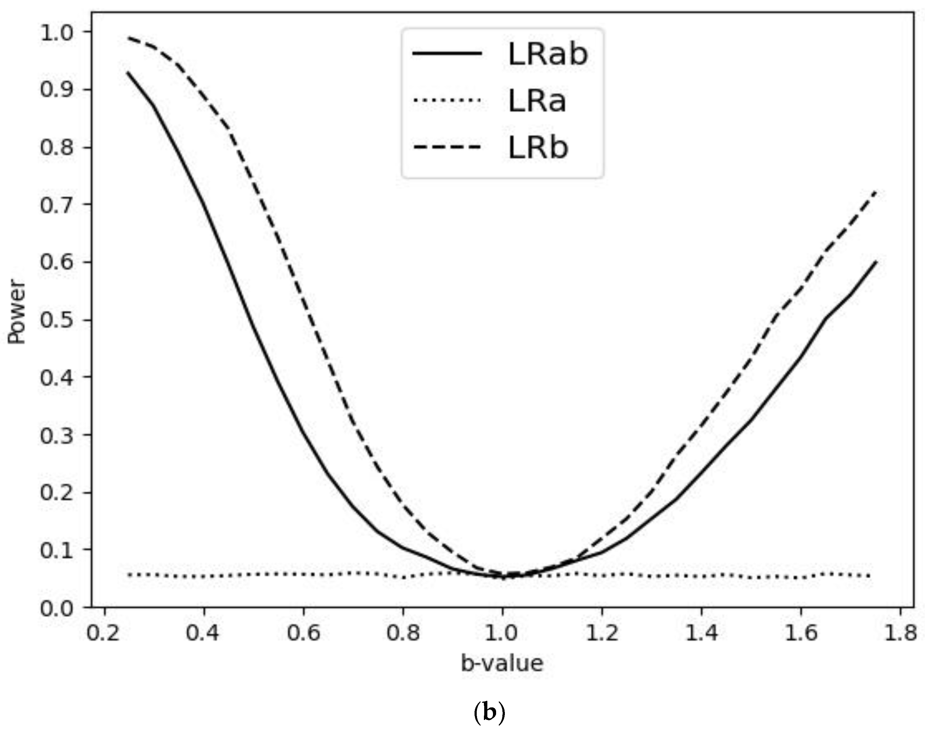
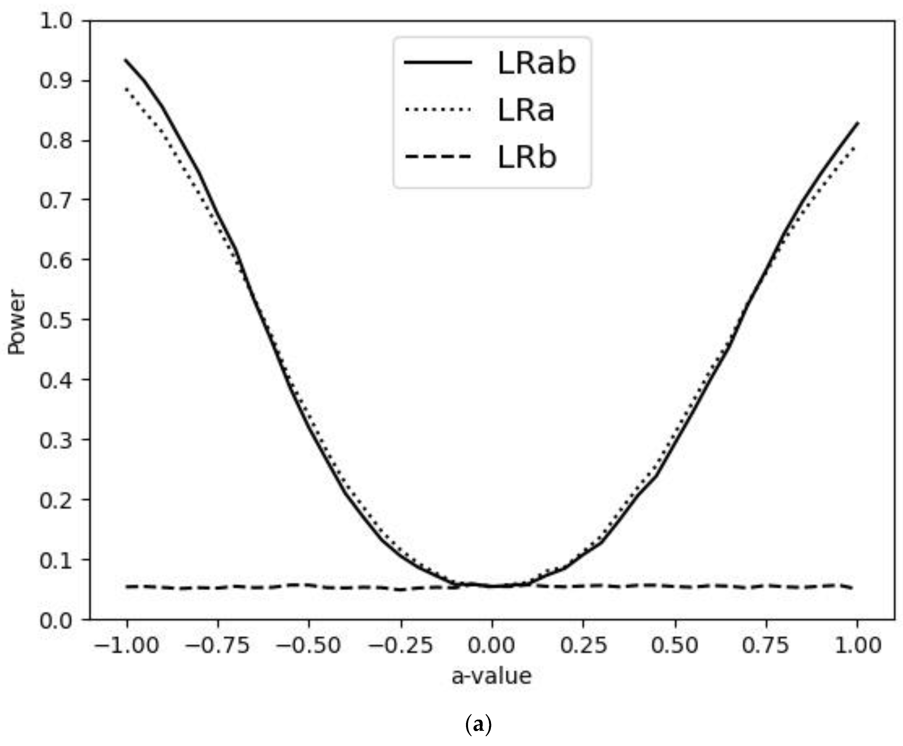
Figure 1. (a) The power curve for b = 1 for sample size $N=50$, where the values of $a$ are on the horizontal axis. (b) The power curve for $a=0$ for sample size $N=50$, where the values of $b$ are on the horizontal axis.

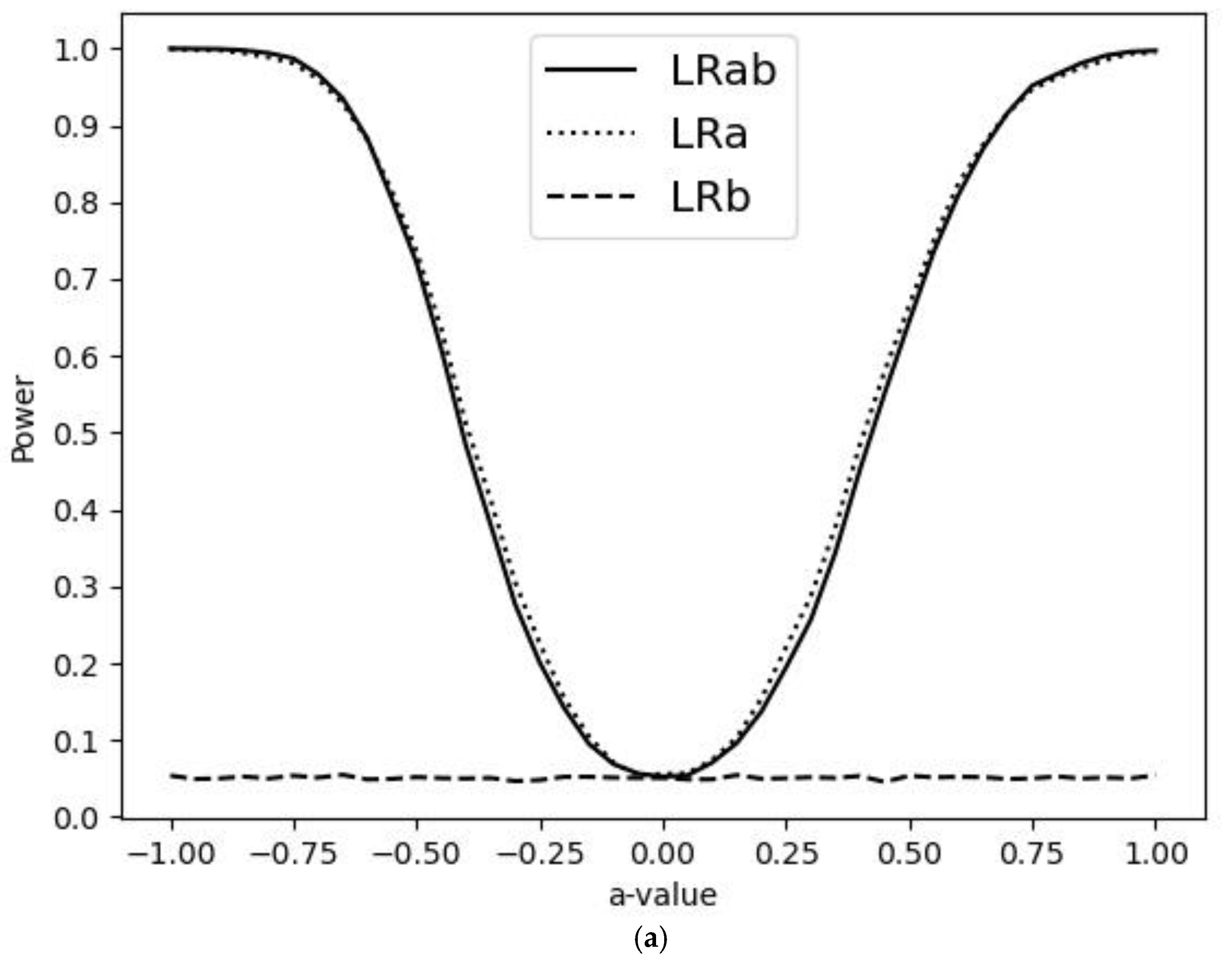
Figure 2. (a) The power curve for b = 1 for sample size $N=100$, where the values of $a$ are on the horizontal axis. (b) The power curve for $a=0$ for sample size $N=100$, where the values of $b$ are on the horizontal axis.

Figure 3. (a) The power curve for b = 1 for sample size $N=250,$ where the values of $a$ are on the horizontal axis. (b) The power curve for $a=0$ for sample size $N=250$, where the values of $b$ are on the horizontal axis.

Figure 1a presents the power plots of the three LR tests for the case that $b=1$ and the sample size is $N=50$, with different values of $a$ on the horizontal axis. Figure 1b presents the power plots of the three LR tests for the case that $a=0$ and the sample size is $N=50$, with different values of $b$ on the horizontal axis. Note that, for typical applications in marketing research, consumer choice modeling, transportation choice, and more, the sample size $N=50$ can be considered as quite small.

Figure 1a,b show that, even already for this small sample, the empirical size is appropriately close to 5%, and the power increases with further away $a$ and $b$ values, respectively. Furthermore, we see that the LRab test has less power than the LRb test when the true $\alpha =0$. However, the loss in power for the LRab test is very small compared to the LRb test when the true $\beta =1$.

Figure 2a,b consider the same settings, but now for sample size $N=100$, whereas Figure 3a,b concern the sample size $N=250$. Comparing these figures with those in Figure 1a,b, where we looked at sample size N = 50, we see that the power curve of the tests rapidly shows steepness with increasing sample size, and hence quickly converges to 1.

4. Illustration

As an illustration, we consider an optical scanner panel data set on purchases of four brands of saltine crackers in the Rome (Georgia) market, collected by Information Resources Incorporated. The data set contains 3292 purchases of crackers made by 136 households over about two years. The data are also analyzed in Chapter 6 of [4] (the data are available from the authors, and the code amounts to a standard module on multinomial logit model estimation). The brands are called Private label, Sunshine, Keebler, and Nabisco. For each purchase, we have the actual price of the purchased brand, the shelf price of the other brands and four times two dummy variables which indicate whether the brands were on display or featured. To describe brand choice, we consider the conditional logit model, where we include as explanatory variables per category the price of the brand and three 0/1 dummy variables indicating whether a brand was on display only or featured only or jointly on display and featured. To allow for out-of-sample evaluation of the model, we holdout the last purchases of each household from the estimation sample. Hence, we have 3156 observations for parameter estimation and use the estimated model to provide 136 forecast probabilities for the out-of-sample purchases. So, $J=4$ and $N=136$.

We obtain the following LR test values:

LRab = 1.67

LRa = 1.57

LRb = 0.06

which suggests that the predicted probabilities from our MNL model do not entail biased forecasts.

When we allow for four different $\beta$ values, that is, as in (10), we obtain the LR test values

LRab = 2.22

LRa = 3.24

LRb = 2.83

Again, we see that the MNL model, as specified in [4], delivers unbiased forecasts. Hence, both models provide unbiased forecasts.

5. Conclusions

We have proposed a simple to implement Likelihood Ration (and Wald) test for forecast bias in case the predictions concern probabilities on independent multinomial outcomes. The test is independent from the origin of the predictions. With simulations, we have shown that the test has proper empirical size and that the empirical power quickly increases with growing sample size. An illustration showed the ease of use of the test.

References

1. de Jong, V.M.T.; Eijkemans, M.J.C.; van Calster, B.; Timmerman, D.; Moons, K.G.M.; Steyerberg, E.W.; van Smeden, M. Sample size consideration and predictive performance of multinomial logistic prediction models. Stat. Med. 2019, 38, 1601–1619. [Google Scholar] [CrossRef] [PubMed]
2. Mincer, J.; Zarnowitz, V. The evaluation of economic forecasts. In Economic Forecasts and Expectations; Mincer, J., Ed.; National Bureau of Economic Research: New York, NY, USA, 1969. [Google Scholar]
3. Franses, P.H. Testing for bias in forecasts for independent binary outcomes. Appl. Econ. Lett. 2021, 28, 1336–1338. [Google Scholar] [CrossRef]
4. Franses, P.H.; Paap, R. Quantitative Models in Marketing Research; Cambridge University Press (CUP): Cambridge, UK, 2001. [Google Scholar]
Disclaimer/Publisher’s Note: The statements, opinions and data contained in all publications are solely those of the individual author(s) and contributor(s) and not of MDPI and/or the editor(s). MDPI and/or the editor(s) disclaim responsibility for any injury to people or property resulting from any ideas, methods, instructions or products referred to in the content.
Article Metrics
Citations
Article Access Statistics
Multiple requests from the same IP address are counted as one view.