Evaluating the Potential of Copulas for Modeling Correlated Scenarios for Hydro, Wind, and Solar Energy

Abstract

The increasing global adoption of variable renewable energy (VRE) sources has transformed the use of forecasting, scenario planning, and other techniques for managing their inherent generation uncertainty and interdependencies. What were once desirable enhancements are now fundamental requirements. This is more prominent in Brazil, given the large hydro capacity that has been installed. Given the need to understand the interdependencies within variable renewable energy systems, copula-based techniques are receiving increasing consideration. The objective is to explore and model the correlation and complementarity, based on the copula approach, evaluating the potential of this methodology considering a case test composed of hydro, wind, and solar assets. The proposed framework simulated joint scenarios for monthly natural energy (streamflows transformed into energy), wind speed and solar radiation, applied to a small case test, considering historical data from the Brazilian energy system. The results demonstrate that simulated scenarios are validated by their ability to replicate key statistical attributes of the historical record, as well as the interplay and complementarity among hydrology, wind speed, and solar radiation.

1. Introduction

The extensive worldwide insertion of variable renewable energy (VRE) adds complexity to all processes related to power systems, such as modeling, planning, operation, and commercialization. The increasing integration of variable renewable energy (VRE), both through large- scale wind and solar photovoltaic (PV) installations and smaller distributed generation units, presents distinct integration challenges for existing power systems. The inherent randomness of VRE generation, its seasonal fluctuations, its spatial and temporal dependencies, high short-term variability, and limitations in data availability [1] are key obstacles that must be overcome.

The global renewable energy market expansion remains strong, led by solar PV. According to 2023 figures, solar PV accounted for two-thirds of the increase in global renewable capacity. This includes both large utility-scale and small distributed systems. The onshore wind capacity expansion registered an all-time record of additions after two consecutive years of decline, rebounding by 70% in 2023 to 107 GW [2]. The capacity increase in Brazil is following the global trend and presenting an accelerated growth rate. It is primordial to improve and develop new methodologies to deal with the uncertainties inherent to VREs in the long-, medium-, and short-term horizons. In the past, only a handful of countries that had reached an advanced stage of large-scale hydro development, such as Brazil, Canada, Norway, and the USA, confronted some of these challenges related to the stochastic analysis of water inflows and the optimization of hydro-thermal operation [3,4,5,6].

Brazil has a natural vocation for renewable generation; 78% of the current capacity installed is supported by renewable sources and approximately 89% of the total electricity generated in 2023 came from renewable generation [7].

The new energy framework, significantly characterized by fluctuating renewable energy, must effectively address the irregular output of variable renewable energy (VRE). Predictive tools offer a viable approach to reduce this issue and manage uncertainty. Multiple forecasting methodologies designed for specific purposes and timeframes are essential for VRE generation. Furthermore, the impact of weather and climate events on VREs results in noticeable spatial and temporal interdependencies. Comprehending the benefits of VRE complementarity is essential, especially considering the rise of blended generation systems incorporating diverse VRE technologies, including hydro, solar, and wind resources, distributed across large areas. Despite the increase in studies examining dependence and complementarity, this topic has been under scrutiny since the initial stages of VRE development [8].

In Brazil, the combination of the power system based on hydro generation and the increase in wind and solar generation amplifies the stochastic nature of the system, bringing more uncertainties and challenges to operation and commercialization. The Brazilian energy system’s operation and commercial framework are supported by a set of computational models that address the problem from different time horizons. The NEWAVE [9], an optimization model based on stochastic dual dynamic programming on a monthly basis, performs a key function in operation optimization and market pricing. The model considers the inflow stochasticity, and it is part of the official model chain used by the Brazilian National System Operator (ONS) and Electrical Energy Trading Chamber (CCEE). Given the current model restrictions, wind and solar generation are modeled deterministically in the NEWAVE, based on the generation of the last five years. Given that wind and solar generation accounted for more than 20% of the generated energy in 2023, the simplified representation of wind and solar generation in the model could harm the operation optimization process and also brings a lot of difficulties for generation companies in managing the risk and revenues related to these assets, taking into account the barriers to simulating scenarios correlated to the NEWAVE model outputs, mainly the link between asset generation and future price scenarios. The innovative scenario generation framework detailed in this article for renewable energy sources, based on official dispatch model outputs, is a key contribution. This advance will enhance analytical capabilities and decision-making for risk management and commercial strategies associated with renewable assets, ultimately contributing to the Brazilian Energy Market’s improved performance. Copula models have garnered significant interest in addressing the challenges of stochastic dependence modeling for renewable energy sources. These models are utilized to capture spatial correlations among geographically dispersed plants powered by the same renewable resource and to quantify the interdependence between different renewable sources, regardless of their geographical proximity [8,10,11,12,13,14]. The complementarity of mixed hydro and wind generation portfolios has been studied in [15]. Further research, including [16,17], has evaluated the potential of integrating wind farms and hydroelectric facilities, specifically in the context of the Brazilian power grid. Additionally, stochastic simulation models are proposed in [18,19,20] to explore various complementary effects and the impact of climatic variables on renewable energy generation.

This work aims to evaluate the potential of copulas to model the spatial and time complementarity between hydro, wind, and solar generation in Brazil through a case test considering actual data. The study, based on copula methodology and in the current Brazilian Electricity Market framework, aims to produce correlated scenarios of future generation for each renewable source: hydro, wind, and solar. The proposed approach is to apply the copula theory, using vine copulas to model complex dependence structures by breaking down the dependence into a series of bivariate copulas, modeling the dependence between hydrology, wind speed, and solar radiance time series. In summary, the objective of this article is to address the following research questions:

• How effectively can copula-based methods model the complex dependency structures (including correlations and complementarities) between hydro, wind, and solar renewable energy resources in the context of the Brazilian energy system?
• To what extent do the joint scenarios for monthly natural energy inflows, wind speed, and solar radiation generated using a copula-based approach accurately reproduce the statistical properties (including extreme events and variability) of historical data?
• How robust are copula-based models for representing the interdependencies between hydro, wind, and solar resources across different regions within Brazil with varying climatological characteristics?
• How do we construct a link between the inflows scenarios, generated by official dispatch models from the existing Brazilian Electricity Market framework, and the scenarios for wind and solar power plants generated by the proposed copula-based model?

The outcomes from the case test show that simulated scenarios can preserve the statistical features of historical data and the spatial and time dependence between hydrological, wind, and solar regimes in some of the considered regions, demonstrating the potential of copulas to model the correlation and complementarity between different renewable sources installed in different regions.

The proposed framework provides valuable insights for estimating constrained off, a condition where generation is limited by technical or operational constraints. The copula-based approach identifies scenarios with restricted generation by modeling the dependence and complementarity between hydrological, wind, and solar resources. This aids system operators and market agents in risk management and developing strategies to mitigate economic losses associated with renewable generation uncertainty.

This article is organized as follows: Section 1 presented above is an introduction, illustrating the problem and the motivation to address it; Section 2 brings the methodological aspects and the proposed framework; Section 3 describes the case test used in this study and the historical data analysis; Section 4 details the estimated model, main results and analysis; and finally, Section 5 discusses this study’s main conclusion and potential future research directions.

2. Methodological Approach

2.1. Copulas—Brief Introduction

Copulas are mathematical functions that couple marginal distributions to their joint distributions. In simpler terms, they are a way to describe the dependence structure between different variables, separate from their individual distributions. Copulas allow the modeling of complex dependencies that traditional linear correlation cannot capture. For example, they can model situations where variables are highly correlated in the distribution’s tails but not in the middle. The copula approach process permits the dependence structure and the individual distributions to be modeled independently, offering more flexibility. This flexibility enables a wide range of applications, and numerous examples can be found in the literature in finance (modeling asset prices), insurance (modeling risks), engineering (modeling system failures), and other fields. The work [21] presents clear definitions, fundamental relationships, and examples of copula theory.

A d-dimensional copula is a Cumulative Distribution Function (CDF) with uniform marginals (1).

$$C:{[0,1]}^d\to [0,1]$$

(1)

Given that C is a distribution function, the following properties are expected:

• CDFs are always increasing, $C\left(\mathbf{u}\right)=C(u_1,\dots ,u_d)$ is increasing in each component $u_i$;
• The marginal in component i is obtained by setting $u_j=1$ for all $j\ne i$ and it must be uniformly distributed $C(1,\dots ,u_i,1,\dots ,1)=u_i$;
• For $a_i\le b_i$, the probability $P(U_1\in [a_1,b_1],\dots ,U_d\in [a_d,b_d])$ must be non-negative, which leads to the so-called $rectangule$ $inequality$
  ${\sum }_{i_1=1}^2\dots {\sum }_{i_d=1}^2{(-1)}^{i_1+\dots +i_d}C(u_{1,i_1},\dots ,u_{d,i_d})$, where $u_{j,1}=a_j$ and $u_{j,2}=b_j$.

A diversity of copulas, called copula families, can be useful for constructing stochastic models capturing different proprieties such as heavy tails, asymmetries, etc. There is extensive literature regarding the copula theory and its use [22,23,24].

As mentioned in [25], dealing with higher-dimensional copulas is not a simple problem. While there are a huge number of parametric bivariate copulas, for higher-dimensional copulas, this number is low. The decomposition of the multivariate in a copula pair poses a more flexible and intuitive approach to dealing with higher dimensions.

The article [26] introduces a new graphical model for dependent random variables, nominated vine. The graphical model (regular vine) is a structure to assist in organizing and dealing with pair-copula constructions (PCCs) [27,28], where for a d-dimensional PCC $d(d-1)/2$, bivariate copulas are arranged in $d-1$ trees. Special subclasses of PCCs called drawable vines (D-vines) and canonical vines (C-vines) are presented in [29]:

• D-vine tree if each node in tree $T-1$ has at most 2 edges. Figure 1 shows a graphical representation for dimension $d=5$.
• In a C-vine tree, the tree $T_i$ has a unique node with $d-1$ edges. The node with $d-1$ edges in tree $T_1$ is called the root. Figure 2 shows a graphical representation for dimension $d=5$.

The C-vine copulas are powerful tools for modeling complex dependencies between multiple variables. The approach decomposes a multivariate distribution into a series of bivariate copulas organized in a hierarchical structure, highlighting a dominant component in the first level of the hierarchy, and the remaining relationships are modeled in subsequent levels. The dominant variable is the central, most connected variable in the first level of the vine structure. The process of determining the dominant variable is not always straightforward, and generally, the following methods are used:

• Empirical Approach: pairwise dependence is measured by Kendall’s tau or Spearman’s rho between all variables (Kendall’s and Spearman’s are both examples of rank correlations. As rank correlations, they possess several advantageous properties compared to linear correlation: (i) independence from marginal distributions; (ii) invariance to strictly increasing non-linear transformations; (iii) always defined; and (iv) bounded range [−1, 1]. They can also be expressed in terms of copulas). The variable exhibiting the strongest overall dependence on others is a potential candidate for the dominant position.
• Model Selection Criteria: information criteria (e.g., Akaike information criterion (AIC), Bayesian information criterion (BIC))are employed to compare different C-vine models, each with a different variable chosen as dominant. The model with the best fit (lowest AIC/BIC) often points to a suitable dominant variable.

The process is to systematically select the bivariate copula family to model the dependence structure accurately between each pair of variables, represented by edges, at each tree of the C-vine, considering the conditional relationships established in preceding trees. The step-by-step selection process is as follows:

• Starting in Tree 1: dominant variable connections.
  • Specify a candidate set of copula families.
  • Estimate the parameters: for each candidate copula, estimate its parameters using the maximum likelihood estimation (MLE) on the data for that pair.
  • Evaluate goodness of fit: employ a model selection criterion, typically AIC or BIC, to compare the fit of the candidate copulas. Lower AIC/BIC values indicate a better fit.
  • Select the best copula: select the copula family with the lowest AIC/BIC for that particular edge.
• Subsequent Trees: conditional dependencies.
  • Move to the next tree, modeling the dependence between two variables conditional on the variable(s) connecting them in the previous tree.
  • For each edge in the trees, carry out the following:

    ‐

    Specify a candidate set of copula families.

    ‐

    Conditional estimation: estimate the copula parameters using MLE. This step requires conditioning the variables linking the pair in the previous tree.

    ‐

    Goodness of fit and selection: as executed for Tree 1, AIC/BIC is used to compare the fit of the candidate copulas and select the copula that presents a better fit.

  • Iterate through trees: this process of copula family selection is replicated for each edge in each subsequent tree of the C-vine structure.

The process, as mentioned above, will be executed in this article using the, version 2.6.0 [30].

2.2. Proposed Framework

To generate correlated scenarios considering different renewable sources using the copula approach, it is necessary to take some steps. The first step is to estimate the marginal distribution for each variable. A goodness-of-fit test was used to determine how well a sample of data fits a theoretical probability distribution; in other words, it assessed whether the observed data could have plausibly come from a specific distribution that was selected. This test is vital for model validation. In this work, the goodness-of-fit test was based on the Kolmogorov–Smirnov (K-S) test. The second step is to define the dependency structure between the variables by a C-vine structure. The third step is to select the copula function for each node of the C-vine structure. The last step is to simulate correlated scenarios for each variable. The general framework is presented in Figure 3.

The energy inflow scenarios, generated from the system’s official model (NEWAVE), will be the basis for generating the correlated scenarios for wind speed and solar irradiance. This will ensure adherence to other important variables, such as difference settlement price, a proxy for spot prices in the Brazilian Energy Market.

3. Case Study

3.1. Case Study Data

To evaluate the potential of copula modeling for generating correlated scenarios for different sources of renewable energy, applied to the Brazilian Power System, a case test was developed.

The Brazilian power system is complex and evolving. Understanding its configuration is crucial for addressing its challenges and capitalizing on its immense renewable energy potential. It is renowned for its vast scale, complex configuration, and heavy reliance on hydroelectric generation. Below is an overview of its key characteristics:

• Hydropower Dominance: Brazil heavily relies on hydroelectric power plants for about 65% of its electricity generation. This makes it one of the world’s leaders in hydroelectric energy.
• Diverse Geography: Hydroelectric plants are spread across the country.
• Large-Scale Plants: like Itaipu (the second largest in the world shared with Paraguay), Tucuruí, and Belo Monte.
• Growing Renewable Sources: While hydropower dominates, Brazil has increasingly incorporated wind power, biomass, and solar energy into its mix. The wind and solar power plants reached 30% of Brazil installed capacity in 2023 [7].
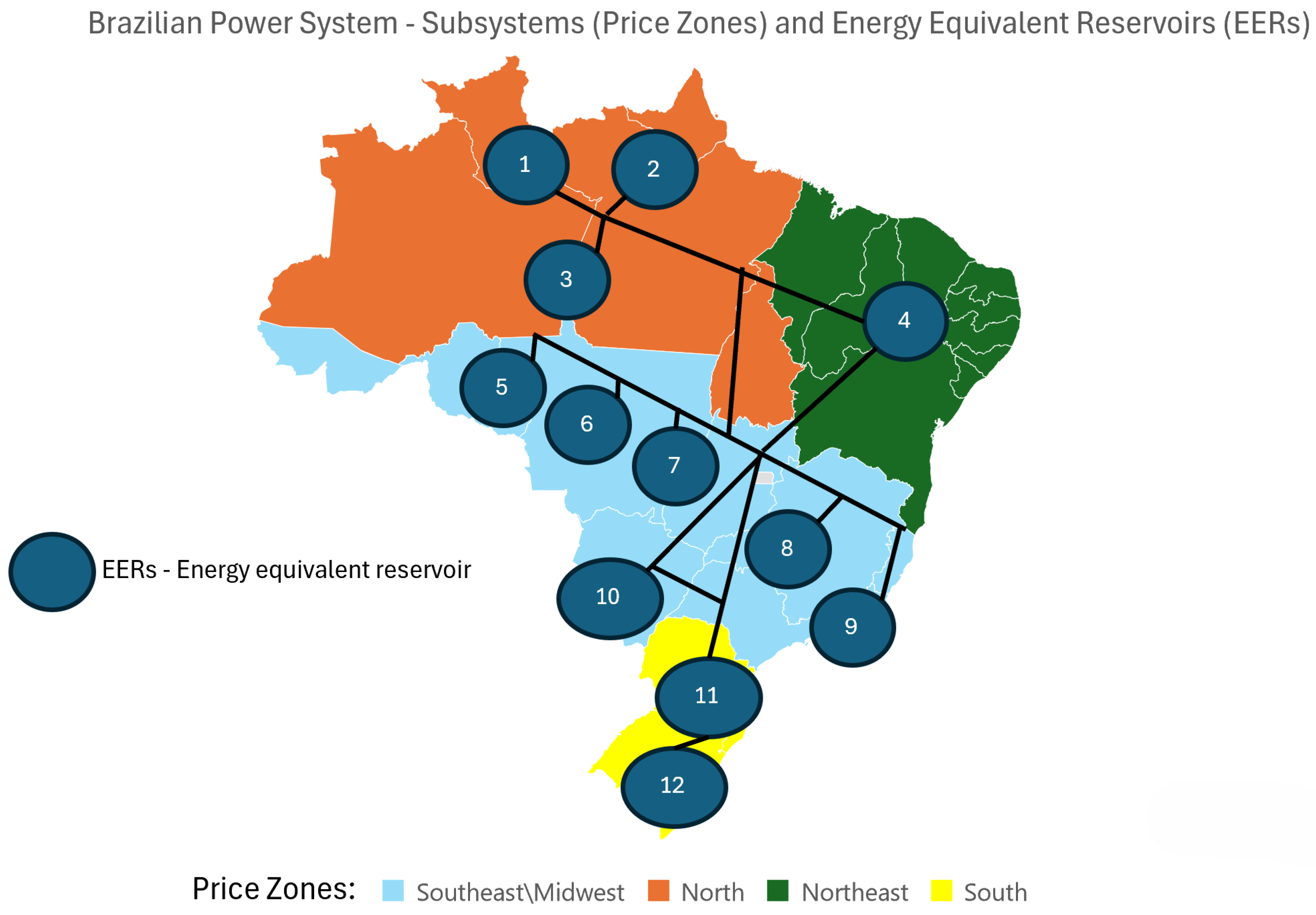
• Vast Transmission Network and Interconnected System: Due to the large distances between some generation centers (like the Amazon basin) and major consumption centers (Southeast), it enables the sharing of energy resources between different regions. The main transmission system, called the basic grid, operating transmission lines from 230 kV to 800 kV, reached 171.640 km in 2023 (source: Brazilian National System Operator (ONS) website).
• Energy Equivalent Reservoir (EER) [31]: Hydropower reservoirs are aggregated, allowing the official model (NEWAVE) to represent the hydropower plants. Currently, there are 12 EERs in the official model used by the Brazilian Operator System (ONS) and Energy Trading Chamber (CCEE).
• Price Zones: the system is divided into 4 subsystems (price zones) South, Southeast/Midwest, Northeast, and North.

The Brazilian power system features a complex dispatch optimization and pricing structure across its various submarkets, reflecting the interplay of generation sources, demand patterns, and regulatory mechanisms. Figure 4 shows the system configuration, divided by the subsystems (price zones) and EERs.

Table 1. Energy Equivalent Reservoirs (EERs)—source: Brazilian National System Operator (ONS).

Number	Energy Equivalent Reservoir (ERR)
1	Manaus
2	Norte
3	Belo Monte
4	Nordeste
5	Madeira
6	Teles Pires
7	Sudeste
8	Paranapanema
9	Paraná
10	Itaipu
11	Sul
12	Iguaçu

lists the 12 EERs.

Brazil has made significant strides in expanding its wind and solar power capacity. The growth is driven by many factors, including high solar irradiation and strong, and consistent winds. Figure 5 shows how the intermittent wind and solar capacity are distributed in the country.

Overall, 75% of the total wind and solar capacity is concentrated in the states of Bahia, Rio Grande do Norte, Piauí, and Minas Gerais, distributed as follows: Bahia 26%, Rio Grande do Norte 24%, Piauí 13%, and Minas Gerais 11%. Locations situated in these states, with a higher installed capacity, were selected to be part of the case study.

The wind speed and solar radiation for the selected locations were collected from the Renewables Ninja Website [33]. The available data came from global reanalysis models and satellite observations. The data sources are as follows:

• NASA MERRA reanalysis [34].
• CM-SAF’s SARAH dataset [35,36].

The case study is composed of three locations with wind speed data in Bahia, Piauí, and Rio Grande do Norte states; three locations with solar irradiance in Minas Gerais, Bahia, and Piauí states; and the historical monthly inflows (42 years), transformed into natural energy inflows, related to Southeast Energy Equivalent Reservoir (EER), according to Figure 6. The Southeast EER contains approximately 41 hydro plants, totaling 10 GW of installed capacity. The hydro plants are distributed among seven states: Tocatins, Goiás, Minas Gerais, Espírito Santo, Rio de Janeiro, São Paulo, and Mato Grosso.

This study covers 42 years, historical data from 1980 to 2022, obtaining a monthly sampling period, totaling 504 observations. A five-year-ahead simulation, aligned with Brazilian Energy Market practices, was performed to evaluate adherence to the proposed method.

3.2. Historical Data Analysis

First, a visual analysis using dispersion graphs is performed. According to the graphics, it is possible to notice the correlation between natural energy inflows, wind speed, and solar irradiance. In general, low values of inflows are correlated with high values of wind speed and solar irradiance. Figure 7 shows the relationship between energy inflows in the Southeast equivalent reservoir and wind speeds in the Bahia, Piauí, and Rio Grande do Norte states, and Figure 8 shows the relationship between energy inflows and solar irradiances in the states of Bahia, Minas Gerais, and Piauí.

The second step is to measure the dependence between variables using Kendall’s $\tau$ rank correlation coefficient. The results show the discordance or negative correlation between energy inflows and other renewable sources, wind speed, and solar irradiance. On the other hand, there is a concordance or positive correlation between wind speed and solar irradiance. Figure 9 shows the observed Kendall’s for January, May, September, and December. May is an exception, where low values of positive correlation between energy inflows and other renewable sources, wind speed, and solar irradiance are presented.

Another important aspect to be investigated is the timing dependence between renewable sources, such as energy inflows, wind speed, and solar irradiance, through cross-correlation analysis. The cross-correlation analysis is used to quantify the similarity between two or more time series as a function of a time lag. It measures how much one time series is linearly related to another at different points in time. Figure 10 reveals the timing dependence between energy inflows from the Southeast equivalent reservoir, the wind speed, and solar irradiance from selected locations.

4. Results

The main objective of this study, given the energy inflow scenarios generated by the NEWAVE model, is to evaluate the performance of the copula approach in generating correlated scenarios for renewable sources, considering hydro, wind, and solar assets.

A five-year-ahead simulation is used to evaluate adherence and performance to the proposed method. The hydrology scenarios produced by the NEWAVE model were used as input for the proposed framework, including 2000 scenarios on a monthly basis from May 2024 to December 2028; the data are an output of the official case from CCEE as of May 2024.

4.1. Estimated Model

4.1.1. Marginal Distribution Estimation

In this study, given that the forward simulation for energy inflows came from NEWAVE, the official model used by ONS and CCEE, it is necessary to estimate the marginals for the wind speed and solar irradiance. The NEWAVE model uses the traditional Periodic Auto-Regressive model (PAR(p)) for energy inflows, and the residuals are modeled using a Log-Normal distribution.

For wind speed, marginal distributions were estimated as a Weibull distribution. According to [37], in absolute terms, the Weibull distribution was the most commonly evaluated and recommended distribution. In summary, 36 distributions were estimated, 12 for each location, considering that 1 distribution was fitted for each month. Figure 11 shows the fitted distributions for April in each location.

The article [38] suggests that Global Horizontal Solar Irradiation (GHI) and Direct Normal Solar Irradiation (DNI) annual series are satisfactorily fitted by Weibull and normal distributions, respectively. It is important to note that the Renewables.Ninja website, the source for the solar data, uses GHI as the primary measurement for solar irradiance. Consequently, this study has followed a parametric approach using the Weibull distribution as the marginal distribution for solar irradiance. Figure 12 shows the fitted distributions for April in each location.

Goodness-of-fit tests based on the Kolmogorov–Smirnov (K-S) test are performed to compare the estimated marginal distributions with observed data, and also assess if the transformed data follow a uniform [0, 1] distribution. The p-values for all tests present values higher than 0.05, indicating that there is not sufficient evidence to reject the null hypothesis. Then, the data could have come from the specified distribution.

4.1.2. C-Vine Structure Assessment

As presented previously, vine copulas are powerful tools for modeling complex dependencies between multiple variables. The general approach decomposes a multivariate distribution into a series of bivariate copulas organized in a hierarchical structure, highlighting a dominant component, which exhibits the strongest overall dependence on other variables, in the first level of the hierarchy, and the remaining relationships are modeled in subsequent levels. The dominant variable is the central, most connected variable in the first level of the vine structure.

Although the energy inflow does not pose as a dominant component, according to the vine copula approach presented above, it is a dominant variable regarding the Brazilian power system, given the importance of this source. It is the only variable modeled stochastically in the official dispatch model (NEWAVE), influencing the spot prices and system operation. Based on this, the energy inflows will be set as the dominant variable in the C-vine structure. It is important to note that it is still necessary to model the other variables’ relationships in subsequent levels, and these relationships will be captured according to the general approach described above.

The C-vine structure was defined according to the following steps:

• The C-vine structure was defined without the energy inflow variable, using the VineCopula Package in R [30], where the root nodes are selected by identifying the node with the strongest dependencies on all other nodes. In other words, given the empirical Kendall’s $\tau$ matrix, the node corresponding to the column that presents the maximum sum is selected. This step is important to model the variables’ relationship from the second level of the C-vine structure and on.
• The energy inflow is set as a dominant variable in the C-vine structure defined in the preceding step, adding a first level to the C-vine structure defined in the previous step.

In this study, 12 C-vine structures are defined, 1 for each month. The variables are represented in Figure 13 and Figure 14 according to

Table 2. Variable representation.

Number	Variable
1	Wind Speed—Bahia
2	Wind Speed—Piauí
3	Wind Speed—Rio Grande do Norte
4	Solar Irradiance—Bahia
5	Solar Irradiance—Minas Gerais
6	Solar Irradiance—Piauí
7	Natural Energy Inflow—Southeast

. Figure 13 shows the C-vine structure, without energy inflow, defining the relationship between wind speeds and solar irradiance; these results were used to set the final C-vine structure. Figure 14 presents the final C-vine structure, where the energy inflow is included as a dominant variable, adding one more level to the structure. Both figures are related to January.

4.1.3. Copula Family Selection

We carefully selected bivariate copulas and identified 252 vine copulas organized into 12 C-vines, each representing a month of the year, and each with 7 variables ($d=7$) and 6 trees ($d-1$), showcasing 21 $\left(d\right(d-1)/2)$ unique copulas per C-vine. Our analysis revealed 28 different copulas, with 86% of nodes assigned a bivariate copula, highlighting various dependencies. Notably, in 27% of cases, the Tawn copula family demonstrated asymmetric tail dependence, revealing different relationships in upper and lower tails. The Clayton family accounted for 13%, indicating lower tail dependence, while the Joe copulas also comprised 13%, capturing positive upper tail dependence. Gumbel copulas represented 12% of the selections, similarly reflecting upper tail relationships, while Frank copulas made up 9%, modeling symmetric dependence. Normal copulas appeared in 7% of cases for symmetric dependencies, and the remaining 6% included t-Student, BB7, and BB8 copulas, highlighting strong tail dependencies and various tail dependence types. These findings open avenues for further exploration of variable relationships and innovative applications across different fields.

Table 3. Percentage of selected bivariate copula families.

T	T_90	T_180	T_270	T2	T2_90	T2_180
1.2%	4.8%	3.2%	2.0%	2.8%	3.6%	2.4%
T2_270	C	C_90	C_270	SC	J	J_90
6.7%	2.8%	3.2%	3.6%	3.2%	4.8%	3.6%
J_270	SJ	G	G_90	G_270	SG	F
1.6%	2.8%	4.8%	2.0%	0.8%	4.4%	9.1%
N	t	BB7	BB7_270	SBB7	BB8_270	SBB8
7.1%	2.8%	0.8%	0.4%	0.4%	0.4%	0.8%

T = Tawn; T_90 = Rotated ${90}^{\circ }$ Tawn; T_180 = Rotated ${180}^{\circ }$ Tawn; T_270 = Rotated ${270}^{\circ }$ Tawn; T2 = Tawn2; T2_90 = Rotated ${90}^{\circ }$ Tawn2; T2_180 = Rotated ${180}^{\circ }$ Tawn2; T2_270 = Rotated ${270}^{\circ }$ Tawn2; C = Clayton; C_90 = Rotated ${90}^{\circ }$ Clayton; C_270 = Rotated ${270}^{\circ }$ Clayton; SC = Survival Clayton; J = Joe; J_90 = Rotated ${90}^{\circ }$ Joe; J_270 = Rotated ${270}^{\circ }$ Joe; SJ = Survival Joe; G = Gumbel; G_90 = Rotated ${90}^{\circ }$ Gumbel; G_270 = Rotated ${270}^{\circ }$ Gumbel; SG = Survival Gumbel; F = FranK; N = Normal; t = t-Student; BB7 = BB7; BB7_270 = Rotated ${270}^{\circ }$ BB7; SBB7 = Survival BB7; BB8_270 = Rotated ${270}^{\circ }$ BB8; SBB8 = Survival BB8.

provides a complete overview of the percentage of each selected copula.

It is important to note that the number of observations in the dataset can significantly influence the copula selection process once copula parameters are estimated from the data, and like most statistical estimations, more data generally lead to more accurate and reliable parameter estimates. With a limited sample size, it might not have enough power to detect subtle or complex dependence structures.

Once the model is estimated, the next step is to perform the simulation and analyze the adherence of the generated scenarios; this step is executed in Section 4.

4.2. Analysis of Simulated Scenarios

The simulation procedure took fifty-two seconds on an IntelCore(TM) i5-8265U with a CPU of 1.60 GHz and 8 GB of RAM. Our approach was implemented in R based on the VineCopula R-Package [30].

4.2.1. Correlation and Complementarity Between Variables

The first analysis is related to the capacity of the proposed framework to reproduce the historical correlation and complementarity between those variables. Figure 15 compares the rank correlation matrix based on Kendall’s $\tau$ from historical and simulated values, considering all data. Figure 16 compares the rank correlation between Southeast energy inflows and wind speed and solar irradiance, on a monthly basis. Generally, the dependency structure between all variables is preserved, but some deviations can be noticed in certain months.

4.2.2. Jointly Simulated Scenarios

It is important to determine whether the jointly forward simulated scenarios for wind speed and solar irradiance, conditioned to energy inflow scenarios generated by the official model NEWAVE, preserved the main characteristics of the observed value. The graphs presented in Figure 17 show that simulated scenarios for wind speed and solar irradiance, conditioned to energy inflow scenarios, maintained the annual seasonal characteristics, and the average of the scenarios is similar to the average of observed values; also, the generated scenarios could reproduce the extreme values.

Another way to compare the simulated scenarios and the historical data is through a box-plot graph, which makes it possible to compare the median; the interquartile range, capturing the spread of the middle of the data; the whiskers, indicating the variability outside the upper and lower quartiles; and the outlier points, significantly far from the rest of the data. Figure 18 shows the box-plots for each month related to wind in the Bahia state, and Figure 19 shows the box-plots related to solar irradiance in the Bahia state. It is possible to notice that the generated scenarios could reproduce the observed data’s main characteristics, showing the proposed framework’s effectiveness.

4.2.3. Cross-Correlation Between Variables

The cross-correlation, in the context of analyzing different variables, measures the similarity between two time series as a function of a time lag applied to one of them, identifying lead–lag relationships between different renewable sources. The simulated scenarios maintained the cross-correlation between the variables; Figure 20 shows the cross-correlation between wind speed in the Bahia state and other variables.

5. Conclusions

The objective of this study is to generate correlated scenarios for different renewable energy sources, focused on the Brazilian power system, creating a link between results from NEWAVE, the official dispatch model used by ONS (Brazilian Independent System Operator) and CCEE (Electrical Energy Trading Chamber), modeling the dependence and complementarity between energy inflows, wind speed, and solar irradiance. The proposed framework uses the copula approach to model the non-linear dependence structure. This research introduces a novel approach by directly linking NEWAVE outputs, the official dispatch model, with tailored scenarios for wind and solar assets. This innovation unlocks new analytical avenues for energy trading and risk mitigation, particularly within the Brazilian Energy Market. The core contribution lies in a framework for renewable energy scenario generation that correlates with official dispatch model data, thus significantly improving decision-making and market performance.

The theme and the proposed approach align with the demand due to the extensive worldwide increase in variable renewable energy which adds complexity to all processes related to power systems, such as modeling, planning, operation, and commercialization. The stochastic nature of the generation, its seasonal aspects, spatial and time dependence, high variability in a short period, and data availability are the main challenges to be addressed. It is primordial to improve and develop new methodologies to deal with the uncertainties inherent to VREs in the long-, medium-, and short-term horizons.

The outcomes show that the proposed framework can simulate scenarios reproducing the statistical features of historical data and the correlation and complementarity among hydrology, wind speed, and solar radiation. The C-vine structure and the selected copulas properly modeled the spatial correlation between variables, and the timing dependence was captured indirectly by the energy inflow scenarios, generated in the NEWAVE model using the periodic autoregressive model, which was the conditional variable, to generate the scenarios for the other variables. The proposed framework emerges as an interesting way to improve the current modeling, helping to understand the nuances of the dependence and complementarity between renewable sources. Also, it poses as a tool to explain the complex interaction of factors within and across submarkets and different generation assets, which requires careful analysis and strategic decision-making to navigate price risks and opportunities.

The results demonstrate the potential of the proposed framework to support operational and commercial decision-making in the Brazilian power system, particularly in integrating hybrid renewable portfolios and risk management under high renewable penetration. The framework’s reliance on historical data limits its ability to capture emerging patterns in renewable generation under extreme climate events, suggesting a need for real-time data integration in future iterations. Monthly discretization is insufficient to describe the complexity of the intermittency of renewable sources and daily patterns.

Future work related to this theme could include the influence of climate phenomena, such as the El Niño–Southern Oscillation (ENSO) and its different phases (El Niño, La Niña, and Neutral), on the forecasting of VREs and the generation of correlated scenarios.

References

1. Brouwer, A.S.; van den Broek, M.; Seebregts, A.; Faaij, A. Impacts of large-scale Intermittent Renewable Energy Sources on electricity systems, and how these can be modeled. Renew. Sustain. Energy Rev. 2014, 33, 443–466. [Google Scholar] [CrossRef]
2. International Energy Agency (IEA). Renewable Energy Market Update—June 2023; IEA: Paris, France, 2023. [Google Scholar]
3. de Queiroz, A.R. Stochastic hydro-thermal scheduling optimization: An overview. Renew. Sustain. Energy Rev. 2016, 62, 382–395. [Google Scholar] [CrossRef]
4. Souza, R.C.; Marcato, A.L.M.; Dias, B.H.; Oliveira, F.L.C. Optimal operation of hydrothermal systems with Hydrological Scenario Generation through Bootstrap and Periodic Autoregressive Models. Eur. J. Oper. Res. 2012, 222, 606–615. [Google Scholar] [CrossRef]
5. Oliveira, F.L.C.; Souza, R.C.; Marcato, A.L.M. A time series model for building scenarios trees applied to stochastic optimisation. Int. J. Electr. Power Energy Syst. 2015, 67, 315–323. [Google Scholar] [CrossRef]
6. de Castro, C.M.; Marcato, A.L.; Souza, R.C.; Junior, I.C.S.; Oliveira, F.L.C.; Pulinho, T. The generation of synthetic inflows via bootstrap to increase the energy efficiency of long-term hydrothermal dispatches. Electr. Power Syst. Res. 2015, 124, 33–46. [Google Scholar] [CrossRef]
7. EPE. Balanço Energético Nacional. 2024. Available online: https://www.epe.gov.br/pt/publicacoes-dados-abertos/publicacoes/balanco-energetico-nacional-ben (accessed on 10 June 2024).
8. Iung, A.M.; Cyrino Oliveira, F.L.; Marcato, A.L.M. A review on modeling variable renewable energy: Complementarity and spatial–temporal dependence. Energies 2023, 16, 1013. [Google Scholar] [CrossRef]
9. CEPEL NEWAVE—Manual do Usuário. 2022. Available online: https://www.cepel.br/wp-content/uploads/2024/10/ManualUsuario-2.pdf (accessed on 10 June 2024).
10. Baboli, P.T.; Brand, M.; Lehnhoff, S. Stochastic Correlation Modelling of Renewable Energy Sources for Provision of Ancillary Services using Multi-dimensional Copula Functions. In Proceedings of the 2021 11th Smart Grid Conference (SGC), Tabriz, Iran, 7–9 December 2021; pp. 1–6. [Google Scholar] [CrossRef]
11. Papaefthymiou, G.; Kurowicka, D. Using Copulas for Modeling Stochastic Dependence in Power System Uncertainty Analysis. IEEE Trans. Power Syst. 2009, 24, 40–49. [Google Scholar] [CrossRef]
12. Zhao, M.; Wang, Y.; Wang, X.; Chang, J.; Zhou, Y.; Liu, T. Modeling and simulation of large-scale wind power base output considering the clustering characteristics and correlation of wind farms. Front. Energy Res. 2022, 10, 810082. [Google Scholar] [CrossRef]
13. de Almeida Pereira, G.A.; Veiga, Á. Periodic Copula Autoregressive Model Designed to Multivariate Streamflow Time Series Modelling. Water Resour. Manag. 2019, 33, 3417–3431. [Google Scholar] [CrossRef]
14. de Almeida Pereira, G.A.; Veiga, Á. PAR(p)-vine copula based model for stochastic streamflow scenario generation. Stoch. Environ. Res. Risk Assess. 2018, 32, 833–842. [Google Scholar] [CrossRef]
15. Denault, M.; Dupuis, D.; Couture-Cardinal, S. Complementarity of hydro and wind power: Improving the risk profile of energy inflows. Energy Policy 2009, 37, 5376–5384. [Google Scholar] [CrossRef]
16. Ávila R., L.; Mine, M.R.; Kaviski, E.; Detzel, D.H.; Fill, H.D.; Bessa, M.R.; Pereira, G.A. Complementarity modeling of monthly streamflow and wind speed regimes based on a copula-entropy approach: A Brazilian case study. Appl. Energy 2020, 259, 114127. [Google Scholar] [CrossRef]
17. Ávila, L.; Mine, M.R.; Kaviski, E.; Detzel, D.H. Evaluation of hydro-wind complementarity in the medium-term planning of electrical power systems by joint simulation of periodic streamflow and wind speed time series: A Brazilian case study. Renew. Energy 2021, 167, 685–699. [Google Scholar] [CrossRef]
18. de Andrade Melo, G.; Oliveira, F.L.C.; Maçaira, P.M.; Meira, E. Exploring complementary effects of solar and wind power generation. Renew. Sustain. Energy Rev. 2025, 209, 115139. [Google Scholar] [CrossRef]
19. Melo, G.; Barcellos, T.; Ribeiro, R.; Couto, R.; Gusmão, B.; Oliveira, F.L.C.; Maçaira, P.; Fanzeres, B.; Souza, R.C.; Bet, O. Renewable energy sources spatio-temporal scenarios simulation under influence of climatic phenomena. Electr. Power Syst. Res. 2024, 235, 110725. [Google Scholar] [CrossRef]
20. Huang, X.; Maçaira, P.M.; Hassani, H.; Cyrino Oliveira, F.L.; Dhesi, G. Hydrological natural inflow and climate variables: Time and frequency causality analysis. Phys. A Stat. Mech. Appl. 2019, 516, 480–495. [Google Scholar] [CrossRef]
21. McNeil, A.J.; Frey, R.; Embrechts, P. Quantitative Risk Management: Concepts, Techniques and Tools-Revised Edition; Princeton University Press: Princeton, NJ, USA, 2015. [Google Scholar]
22. Jaworski, P.; Durante, F.; Hardle, W.K.; Rychlik, T. Copula Theory and Its Applications; Springer: Berlin/Heidelberg, Germany, 2010; Volume 198. [Google Scholar]
23. Charpentier, A.; Fermanian, J.D.; Scaillet, O. The estimation of copulas: Theory and practice. Copulas Theory Appl. Financ. 2007, 35. [Google Scholar]
24. Xu, H.; Chen, J.; Lin, H.; Yu, P. Unraveling Financial Interconnections: A Methodical Investigation into the Application of Copula Theory in Modeling Asset Dependence. Eur. Acad. J. 2024, 1. [Google Scholar]
25. Aas, K.; Czado, C.; Frigessi, A.; Bakken, H. Pair-copula constructions of multiple dependence. Insur. Math. Econ. 2009, 44, 182–198. [Google Scholar] [CrossRef]
26. Bedford, T.; Cooke, R.M. Vines—A new graphical model for dependent random variables. Ann. Stat. 2002, 30, 1031–1068. [Google Scholar] [CrossRef]
27. Bedford, T.; Cooke, R.M. Probability density decomposition for conditionally dependent random variables modeled by vines. Ann. Math. Artif. Intell. 2001, 32, 245–268. [Google Scholar] [CrossRef]
28. Kurowicka, D.; Cooke, R. Distribution-free continuous Bayesian belief. Mod. Stat. Math. Methods Reliab. 2005, 10, 309. [Google Scholar]
29. Kurowicka, D.; Cooke, R.M. Uncertainty Analysis with High Dimensional Dependence Modelling; John Wiley & Sons: Hoboken, NJ, USA, 2006. [Google Scholar]
30. Nagler, T.; Schepsmeier, U.; Stoeber, J.; Brechmann, E.C.; Graeler, B.; Erhardt, T.; Almeida, C.; Min, A.; Czado, C.; Hofmann, M.; et al. Vinecopula: Statistical Inference of Vine Copulas. 2023. Available online: https://cran.r-project.org/web/packages/VineCopula/VineCopula.pdf (accessed on 10 June 2024).
31. Arvanitidits, N.V.; Rosing, J. Composite Representation of a Multireservoir Hydroelectric Power System. IEEE Trans. Power Appar. Syst. 1970, PAS-89, 319–326. [Google Scholar] [CrossRef]
32. Agência Nacional de Energia Elétrica—ANEEL. 2023. Available online: https://www.gov.br/aneel/pt-br (accessed on 10 June 2024).
33. Staffell, I.; Pfenninger, S. Renewables.Ninja. 2016. Available online: https://www.renewables.ninja (accessed on 5 October 2018).
34. Rienecker, M.M.; Suarez, M.J.; Gelaro, R.; Todling, R.; Bacmeister, J.; Liu, E.; Bosilovich, M.G.; Schubert, S.D.; Takacs, L.; Kim, G.K.; et al. MERRA: NASA’s modern-era retrospective analysis for research and applications. J. Clim. 2011, 24, 3624–3648. [Google Scholar] [CrossRef]
35. Müller, R.; Pfeifroth, U.; Träger-Chatterjee, C.; Trentmann, J.; Cremer, R. Digging the METEOSAT Treasure—3 Decades of Solar Surface Radiation. Remote Sens. 2015, 7, 8067–8101. [Google Scholar] [CrossRef]
36. Müller, R.; Pfeifroth, U.; Träger-Chatterjee, C.; Cremer, R.; Trentmann, J.; Hollmann, R. Surface Solar Radiation Data Set—Heliosat (SARAH). 2015. Available online: https://www.cmsaf.eu/en/products/radiation/surface_solar_radiation/sarah_v2/index.html (accessed on 10 June 2024).
37. Jung, C.; Schindler, D. Wind speed distribution selection—A review of recent development and progress. Renew. Sustain. Energy Rev. 2019, 114, 109290. [Google Scholar] [CrossRef]
38. Peruchena, C.M.F.; Ramírez, L.; Silva-Pérez, M.A.; Lara, V.; Bermejo, D.; Gastón, M.; Moreno-Tejera, S.; Pulgar, J.; Liria, J.; Macías, S.; et al. A statistical characterization of the long-term solar resource: Towards risk assessment for solar power projects. Sol. Energy 2016, 123, 29–39. [Google Scholar] [CrossRef]
Figure 1. D-vine tree for d = 5 .
Forecasting 07 00007 g001
Figure 2. C-vine tree for d = 5 .
Forecasting 07 00007 g002
Figure 3. General framework.
Forecasting 07 00007 g003
Figure 4. The Brazilian power system configuration.
Forecasting 07 00007 g004
Figure 5. Wind and solar installed capacity as of September 2023 [32].
Forecasting 07 00007 g005
Figure 6. Case study configuration.
Forecasting 07 00007 g006
Figure 7. Dispersion graphs between energy inflows in the Southeast (axis x) and wind speeds (axis y), in the three locations (Bahia, Piaui, and Rio Grande do Norte). For all locations, it is possible to notice the occurrence of high wind speeds when low inflows occur.
Forecasting 07 00007 g007
Figure 8. Dispersion graphs between energy inflows in the Southeast (axis x) and solar irradiance (axis y), in the three locations (Bahia, Minas Gerais, and Piaui). For all locations, it is possible to notice the occurrence of high solar irradiance when low inflows occur.
Forecasting 07 00007 g008
Figure 9. Observed Kendall’s τ for January, May, September, and December. Inf_SE = energy inflow Southeast; I_PI = solar irradiance Piaui; I_MG = solar irradiance Minas Gerais; I_BA = solar irradiance Bahia; W_RN = wind speed Rio Grande do Norte; W_PI = wind speed Piaui; W_BA = wind speed Bahia.
Forecasting 07 00007 g009
Figure 10. Cross-correlation between energy inflows x wind speed and energy inflows x solar irradiance; analyzing the graphs, it is possible to notice a temporal dependence between energy inflows versus wind speed and solar irradiance for all locations.
Forecasting 07 00007 g010
Figure 11. Marginal distributions—wind speed/April. The blue line shows the historical data and the red line is the adjusted distribution.
Forecasting 07 00007 g011
Figure 12. Marginal distributions—solar irradiance/April. The blue line shows the historical data and the red line is the adjusted distribution.
Forecasting 07 00007 g012
Figure 13. Previous C-vine structure, without energy inflow variable.
Forecasting 07 00007 g013
Figure 14. Final C-vine structure, including energy inflow variable.
Forecasting 07 00007 g014
Figure 15. Historical x simulated Kendall’s τ . Inf_SE = energy inflow Southeast; I_PI = solar irradiance Piaui; I_MG = solar irradiance Minas Gerais; I_BA = solar irradiance Bahia; W_RN = wind speed Rio Grande do Norte; W_PI = wind speed Piaui; W_BA = wind speed Bahia.
Forecasting 07 00007 g015
Figure 16. Each graph shows the historical x simulated Kendall’s τ for energy inflow x wind and solar renewable sources, for some months. Blue bars: historical Kendall’s τ ; red bars: simulated Kendall’s τ .
Forecasting 07 00007 g016
Figure 17. Wind speed and solar irradiance scenarios for the 6 locations. The grey lines represent the simulated scenarios, the white lines are historical values, the red dotted line represents the simulated scenarios average, and the blue dotted line is the historical average.
Forecasting 07 00007 g017
Figure 18. Box-plots: wind speed.
Forecasting 07 00007 g018
Figure 19. Box-plots: solar irradiance.
Forecasting 07 00007 g019
Figure 20. Cross-correlation between wind speed (Bahia state) and other variables.
Forecasting 07 00007 g020