Precision and Reliability of Forecasts Performance Metrics

Abstract

The selection of an accurate performance metric is highly important to evaluate the quality of a forecasting method. This evaluation may help to select between different forecasting tools of forecasting outputs, and then support many decisions within a company. This paper proposes to evaluate the sensitivity and reliability of forecasts performance metrics. The methodology is tested using multiple time series of different scales and demand patterns, such as intermittent demand. The idea is to add to each series a noise following a known distribution to represent forecasting models of a known error distribution. Varying the parameters of the distribution of the noise allows to evaluate how sensitive and reliable performance metrics are to changes in bias and variance of the error of a forecasting model. The experiments concluded that sRMSE is more reliable than MASE in most cases on those series. sRMSE is especially reliable for detecting changes in the variance of a model and sPIS is the most sensitive metric to the bias of a model. sAPIS is sensible to both variance and bias but is less reliable.

1. Introduction

The forecasting community has long been searching for the best method to assess the performance of forecasting models. In many industrial applications, such as retail, forecasting performance must be aggregated to avoid the high complexity of analyzing performance for every single product [1]. In this case, it is important to assess the performance of models in the best possible way, since it will translate into actual and/or opportunity losses [2].

In addition, in some cases, demand comes in an intermittent or erratic fashion [3]. This type of demand presents a high number of consecutive null demands, or it can be characterized with a high coefficient of variation [4]. These cases present a challenge in measuring the performance of forecasting models due to the high number of null demands [5], which can cause some performance metrics to be undefined. In these situations, it is nevertheless possible to use a specific metric (MAAPE) developed by [6], which considers the evaluation of errors as an angle, instead of a ratio. MAAPE permits to solve the problem of MAPE when dealing with zero or close to zero values to predict. With MAPE these values lead to undefined of infinite evaluations. The arctangent calculation added in MAAPE permits to prevent those undefined and infinite situations. MAAPE overcomes the problem of division by zero and at the same time preserves the philosophy and properties of MAPE [6].

More recently, [7] showed that the best forecasting techniques at the last M competition presented a small difference in performance. Therefore, correctly identifying the best technique is going to become increasingly difficult as forecasting techniques become closer to perfection. For this reason, it is important to evaluate precisely how the sensitivity and reliability of performance metrics evolve with small variations of errors. This criterion will become an important factor for the selection and ranking of forecasting models. This is without considering manually added adjustments to adjust the outputs of the forecast considering information not present in the models [8], which complicate the interpretation of measurement results.

This search was in part driven to solve the difficulties of forecasting multiple series of different scale and demand patterns, such as intermittent demand [3]. This paper addresses this problem by measuring the sensitivity and reliability of forecasts performance metrics. It presents how variation in bias and variance of the error of a forecasting model influences the performance obtained with a specific metric. This is done by comparing performance across multiple time series of different scale and demand pattern.

The proposed methodology allows to identify what is the most sensitive and reliable performance metric. This is important since the community is aware of the difficulties of selecting appropriate parameters and the best models, especially in the context of intermittent demand [9].

The sections in this paper are divided as follows. Section 2 presents forecasts performance metrics. Section 3 presents the methodology to measure sensitivity and reliability. Section 4 presents the results of the application of the methodology on real data. Finally, Section 5 provides a summary and recommendations based on the empirical results.

2. Forecasts Performance Metrics

The evaluation of forecasts performances is classically measured by their accuracy. The evaluation of the accuracy is essentially based on metrics evaluating the forecast error. The forecast error for period h is defined as: $e_h=Y_h-F_h$, the difference between the current value for period h ($Y_h$) and the forecast for period h ($F_h$).

In a survey on researchers and practitioners, Ref. [2] identified that the reasons for selecting one of the performance metrics or another were related to their ease of interpretation, ease of implementation, and speed of execution. Since the advent of the M forecasting competitions, evaluation methods have become more standardized across the literature, however, Ref. [10] raised, despite this, the lack of theory to decide which metric to use.

Since then, several problems with evaluation metrics have been resolved. In particular, the difficulties of scaling for an aggregated evaluation of the results of series at different scales or, the intermittent cases that often involved divisions by zero or divisions by numbers close to zero. It is partly thanks to the proposals of [11] that these problems are now solved. Ref. [11] divide performance metrics into four types: scale-dependent, percent error-based, relative, and scaled metrics. Ref. [12] propose a fifth type of metric: cumulative metrics.

Ref. [13] explored forecasts performance metrics through empirical comparisons. They measured reliability as being the average Spearman correlation for pairwise comparisons among five different subsample. They recommended Median Absolute Percentage Error (MdAPE) to select the most accurate forecasting method and they also introduced relative based error metrics, such as Relative Absolute Error (RAE). This metric scales the absolute error with the one of a naïve method, but [4] argued that such a metric along with the Mean Absolute Percentage Error (MAPE) were not appropriate for intermittent demand since they could involve division by zero. They were not able to measure it but mentioned the importance of the sensitivity of performance metrics.

To solve problems of relative-based scaling methods, ref. [11] introduced the Mean Absolute Scaled Error (MASE), an adaptation of the relative based metric which scales the error using the in-sample error of a benchmark method instead of the out-of-sample error of a benchmark method.

Ref. [12] studied the case of forecast evaluation for intermittent case. They introduced cumulative methods, such as Period in Stock (PIS) and the Cumulated Forecast Error (CFE), as they are not biased toward zero forecast compared to other classical metrics, such as RMSE and MAD [14].

Then, ref. [15] used the idea proposed by [11] to scale $MSE$, $MAE$, and $PIS$ with the in-sample mean demand instead of the in- sample error of a benchmark method. A similar idea was used in [10] but was critiqued in [11] as the in-sample mean could be skewed in presence of non-stationary data.

The main performance metrics are calculated the following way:

$$MSE=mean\left(e_h^2\right)$$

(1)

$$MAE=mean\left(\right|e_h\left|\right)$$

(2)

$$RMSE=\sqrt{MSE}$$

(3)

$MSE$, $MAE$, and $RMSE$ are metrics whose scale depends on the scale of the time series being evaluated. They do not allow comparison of performance between series.

$$MAPE=mean\left(\right|\frac{e_h}{Y_h}\left|\right)$$

(4)

$$sMAPE=2\frac{|e_h|}{Y_h+F_h}$$

(5)

$MAPE$ and $sMAPE$ are metric whose errors are evaluated as a proportion of the amplitude of the series. These metrics are undefined in the presence of zero amplitude and penalize more the positive errors.

$$MRAE=mean\left(\right|\frac{e_h}{e_h^{bench}}\left|\right)$$

(6)

$$RelMAE=\frac{MAE}{MA{E}^{bench}}$$

(7)

In $MRAE$ and $RelMAE$, $bench$ means that the value was calculated from a reference method, usually a naive method. $MRAE$ and $RelMAE$ are metric whose error or metric are relative to that of a reference method. They have indefinite mean and infinite variance.

$$MASE=mean\left(\frac{|e_h|}{MA{E}_{in-sample}^{bench}}\right)$$

(8)

In $MASE$, the subscript “n-sample” means that the value is calculated on the training data. $MASE$ is a metric whose error is normalized by an in-sample factor. $MASE$ can be biased towards 0.

$$PIS=\sum _{h=1}^H-e_h$$

(9)

Finally, PIP is a metric with cumulative errors. It does not allow to compare performances between series.

The first motivating factor on performance metrics was to find metrics able to compare the performance of models across multiple series of different scales. The second motivating was to ensure definite and stable metrics across all cases that could be met like for the case of intermittent demand.

Although it is now known how to evaluate the aggregate performance of a set of mixed profile series, there is still no theory for choosing the “best” metric. In general, several metrics are used to evaluate the performance of a forecasting model. However, what if the results of the metrics are conflicting? Very few studies have addressed this topic. The studies conducted to compare and guide the choice of metrics have mainly focused on their mathematical properties [11] or on empirical and statistical comparisons between the results of different metrics [12,13]. None of these studies attempted to quantify the precision of the metrics, even though this is stated as an important factor by [13]. Moreover, how can we choose which one to trust more in case of conflicting results? The studies previously cited tell us which metrics are correlated without giving any indication on the reliability and, thus, on the importance to be given to each of them. A solution to this problem is proposed in the following.

3. Methodology

This section presents the methodology used to compare performance metrics according to their sensitivity and reliability. The main idea of the methodology is to build fictitious forecasting models with a chosen error distribution. Then, we evaluate how each performance metric performs to detect each error distribution included.

The methodology is the following:

• Y is the real data that a prediction model M has to predict.
• We define:
  • $\epsilon$ as the prediction error of M,
  • F as the output of the forecasting model M, such that $F=Y+\epsilon$.
• We control $\epsilon$, giving it specific properties.
• We evaluate the performance metrics in terms of sensitivity and reliability, considering that Y (real data) and $\epsilon$ (controlled) are known.

In the following subsections, the different elements of the methodology are explained in detail.

3.1. Controls on $\epsilon$

Considering that F, Y, and $\epsilon$ are time series, we need to specify them at each time period i. For that, we will use:

$$F_{i,h}=Y_{i,h}+{\epsilon }_i$$

(10)

where i represents the index of the time series, h the horizon of the forecast, and ${\epsilon }_i\sim N({\mu }_i,{\sigma }_i^2)$ is the random noise.

The choice of the error distribution could have been any distribution and the following results would still be valid. Indeed, since to measure the performance of a forecasting model on multiple time series, the aggregation of the performance must follow a normal distribution according to the central limit theorem. Thus, to simplify the following analysis, the normal distribution is chosen so that the bias and variance of the error distribution of the forecasting models are directly related to the chosen parameters of the error distribution.

In a case with multiple time series, the parameters of the distribution of the error of a model should consider the different scales of the different series.

To do so, the chosen parameters of the error are coefficients of the in-sample mean value of each series, making the error size relative to the scale of the series.

$${\mu }_i=\alpha \frac{1}{N}\sum _t^N{Y}_{i,t}$$

(11)

$${\sigma }_i=\beta \frac{1}{N}\sum _t^N{Y}_{i,t}$$

(12)

where $\frac{1}{N}{\sum }_t^N{Y}_{i,t}$ is the in-sample mean value of the time series. The parameters $\alpha$ and $\beta$ take values between 0 and 1 so the parameters of the error distribution are equal to a proportion of the in-sample mean.

To summarize, the fictitious forecasting models are composed of the actual value plus a noise that follows a chosen normal distribution. For each fictitious model, the parameters of the error distribution are set to a certain proportion $\alpha$ and $\beta$ of the in-sample mean of each series. This makes the error distribution proportionate to the scale of each series.

This way, one can create multiple fictitious models varying $\alpha$ and $\beta$ in an ordered manner with different increments to measure how sensitive and reliable performance metrics are to detect the difference in bias and variance of the error of different models. In further sections, the models are defined by the parameters of their error distribution which are set to a proportion of the in-sample mean.

3.2. Performance Metrics

For the experiment presented in Section 4, $RMSE$, $sMAPE$, $MASE$, and $PIS$ were chosen since they are all common and known metrics. In addition, they can be, or are, adapted to always be defined and can be scaled using the [15] scaling factor. Additionally, the results by [12] seemed to show that all metrics of the same category are strongly correlated, and for this reason, only one metric of each metric class is used.

Scaled versions of the metrics are used: $RMSE$$\left(sRMSE\right)$, $PIS$$\left(sPIS\right)$ and Absolute $PIS$$\left(sAPIS\right)$. They are scaled to allow comparison of performance across series of different scales. The metrics, along with their scaling factors, are described under:

$$sRMSE=\frac{\sqrt{\frac{1}{H}{\sum }_h^H{e}_h^2}}{\frac{1}{N}{\sum }_t^N{Y}_t}$$

(13)

$$sPI{S}_H=\frac{-{\sum }_h^H{\sum }_{i=1}^h{e}_i}{\frac{1}{N}{\sum }_t^N{Y}_t}$$

(14)

$$sAPI{S}_H=\frac{|{\sum }_h^H{\sum }_{i=1}^h{e}_i|}{\frac{1}{N}{\sum }_t^N{Y}_t}$$

(15)

We used scaled metrics as defined in [15] as it is easy to interpret in practical terms. It will also allow us to measure what is the impact on precision and reliability of using a scaling factor robust to non-stationary data as it is for $MASE$. Finally, the aggregation of results across both time series and different horizons is done by taking the mean. For this reason, an additional “m” was added to the metrics abbreviation so that one can make a distinction between the aggregation of horizon periods and the series aggregation.

In those metrics, the predicted values F are not used, but only the prediction errors $\epsilon$ and the real data Y. The methodology and results do not depend on the prediction model (forecasting tools).

3.3. Sensitivity

Variation of the bias and the standard deviation parameter will reveal how different metrics react to changes of these parameters. This reveals which metric is the most sensitive and potentially the best one to distinguish between two models of similar error distributions.

In the present case, we estimate the sensitivity of a loss function by computing the average variation rate of a loss function estimated at fixed intervals. The details of the computations are described in Section 4.2 (Equation (16)) Section 4.3 (Equation (16)).

The same thing can be done by fixing one parameter for several different values and varying the other one. That will allow one to estimate the influence of each parameter on the other one.

The results will allow one to draw conclusions about the sensitivity of metrics to standard deviation and bias of a model. The second measure of sensitivity presents how stable sensitivity is to one parameter given changing values for the other one.

3.4. Reliability

In this section, reliability is evaluated in terms of ranking of models. Since the real error distribution of the models is known, as defined in Equation (10), we can rank the models exactly. The ranks are obtained by sorting the models according to the parameter of the error distribution that is being varied in an ascending order. So, the ranks obtained with the performance metrics can be compared to the real rank of each model. To test this, different configurations of scales for the bias, the standard deviation and the scale of the variation ($\mathsf{\Delta }\mu$ and $\mathsf{\Delta }\sigma$) between two models are considered.

The different situations are presented in

Table 1. Configurations of standard deviation, bias, and variation standard deviation to test and evaluate the reliability of metrics.

$\mathit{\sigma }$	$\mathit{\mu }$	$\mathbf{\Delta }\mathit{\sigma }$	$\mathbf{\Delta }\mathit{\mu }$
−	−	−	0
+	−	−	0
+	−	+	0
−	+	−	0
+	+	−	0
+	+	+	0

. Since the error is under control, in the experiment, we define parameters $\mu$, $\sigma$, $\mathsf{\Delta }\sigma$, and $\mathsf{\Delta }\mu$ in terms of deviation from original signal. The plus and minus symbols represent the relative order of magnitude of the different parameters in comparison to the others. If $\mu$ (respectively, $\sigma$) has a minus symbol then $\alpha$ in Equation (11) (respectively, $\beta$ in Equation (12)) would be less than 0.01. Otherwise, this would mean they would both be of the order of magnitude of 1% of the in-sample mean. The same applies for $\mathsf{\Delta }\sigma$ and $\mathsf{\Delta }\mu$, which represent the difference in standard deviation and bias of the error distribution of the forecasting models. A minus symbol would indicate $\alpha$ and $\beta$ are two orders of magnitude less than 1% and the plus symbol indicates they are an order of magnitude less than 1%. The $\mathsf{\Delta }$ must be smaller than the parameter so that, once multiplied by the number of models, it reaches the same order of magnitude as the parameter. For example, the (+++0) configuration implies $\sigma ,\mu$ of the order of 1% and $\mathsf{\Delta }\sigma$ of 0.1%. So that $\mathsf{\Delta }\sigma$ multiplied by the number of models is of the order of 1%. The (++−0) configuration would have both parameters of the order of 1% and $\mathsf{\Delta }\sigma$ of 0.01%.

To rank the models exactly given their error distribution, only one of the distribution parameters at a time will vary. So, either the bias of the standard deviation will be fixed, while the other will change. Table 1 presents half the configurations, where the others will consider a variation of bias with fixed standard deviation. Note that there is no configuration where $\sigma$ is small and $\mathsf{\Delta }\sigma$ is large. This is because large variations would bring the interval of $\sigma$ from small to large, making it the same configuration as both $+\sigma$ and $+\mathsf{\Delta }\sigma$.

The idea is to measure, for each configuration of bias, standard deviation and delta, the quality of the ranking rendered by the performance metrics. The quality is obtained by comparing metrics rankings to the real ranking of models.

Two different metrics are used to measure the quality of the rankings. The first one is Spearman’s rank correlation [16]. This metric returns the correlation between the real rank and the rank given by metrics. The measure’s value lies between −1 and 1 to indicate negative to positive perfect correlation. It allows us to make conclusions about the general tendency of metrics to rank models in the same order as real rankings.

The second one is the normalized Discounted Cumulative Gain (nDCG) [17]. This metric provides a score between 0 and 1, 1 being the perfect ranking. The main difference between nDCG and Spearman’s rank correlation is that nDCG gives more importance to ranking models correctly in the firsts rank compared to those in the lasts rank.

Indeed, the nDCG metric provides a relevance score to every model it needs to rank and it discounts the relevance, as it appears lower in the ranking. In this experiment, 1 over the real rank of each model is used as their relevance score. This is especially important given that being right for the ranking of the first N models is of greater importance than showing a similar general tendency, as does Spearman’s rank correlation.

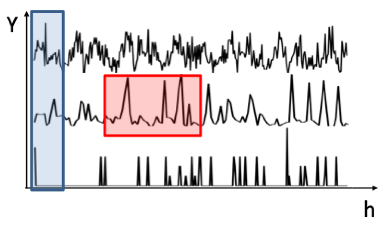
Reliability is observed in function of the number of forecast horizons and the number of series performances used to average performance as illustrated in Figure 1. The figure presents three different series. Its global performance is calculated by varying the number of forecast horizons used to estimate the performance for a series (red square), and by varying the number of series performances that are averaged (blue square).

To make sure the results were not obtained only by chance, this step is repeated 35 times with different series and the results are averaged. The average reliability of all repetitions is finally plotted to visualize the behaviour of the metrics. Thus, the convergence and the general superiority in terms of correlation and nDCG is observed to conclude on the relative reliability of the metrics. So even if some observations of the correlation are not formally significant in a statistical sense, we can still conclude on the overall performance of the metric compared to the others.

4. Results

4.1. Data

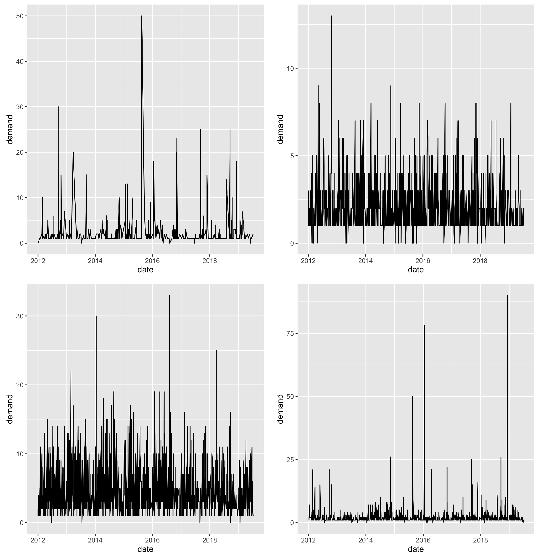
The data used to test the methodology comes from Logistik Unicorp, a company in charge of supplying uniforms to the members of organizations such as the Canadian Army, Canadian Borders, and many other organizations. Several thousand time series were available. Each one represents the demand for an article of clothing in the uniform of a certain size. The demand was aggregated to weekly demand to fit with the MRP system and for other planning purposes. Series with at least two years of demand were kept. That left 23 weeks of horizon periods to evaluate performance on.

Figure 2 shows a couples of series of demand that were used to run the experiment.

4.2. Standard Deviation Sensitivity

To measure the metric’s sensitivity to the standard deviation of a model, the bias of the model was set to $\mu =0$. This leaves only the standard deviation parameter $\sigma$ that was studied through the standard deviation of the distribution, which is equal to $\sigma$. The parameter varied between 1% and 50% of the in-sample mean.

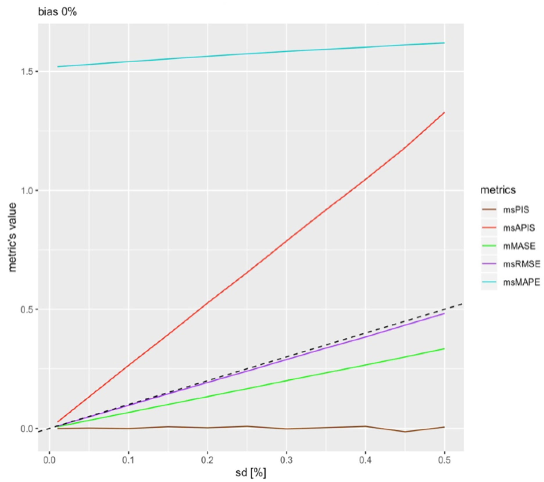
Figure 3 illustrates the global performance of all the metrics values. The dashed line represents the real standard deviation. $msRMSE$ is close to the real standard deviation of the model, which is what is expected by theory. This reassures that the scaling method worked, since the observed trend for $msRMSE$ is almost perfectly aligned with the real value.

All metrics show linear growth. Therefore, the slope of each metric can be approximated with the equation below.

$$vr=mean\left(\frac{L(\sigma +\mathsf{\Delta })-L\left(\sigma \right)}{\mathsf{\Delta }}\right)$$

(16)

where $vr$ is the variation rate, $L\left(\sigma \right)$ is the performance metric expressed in function of standard deviation L and $\mathsf{\Delta }$ is the variation in standard deviation, which is 5% in this case.

This allows conclusions to be drawn on each metric’s sensitivity to standard deviation in absence of bias in forecasting models.

Table 2. Average variation rate of performance metrics for a variation in standard deviation and fixed bias of forecast models.

Metric	msPIS	msAPIS	mMASE	msRMSE	msMAPE
variation rate (vr)	0.01	2.65	0.67	0.96	0.21

represents the variation rate of metrics in Figure 3.

What is important to note is the order of magnitude of the variation more than the values themselves. Indeed, since the values probably vary from one dataset to another and depending on conditions, such as the number of series, the number of forecast horizons, the level of intermittence of the data, etc. $msRMSE$ is the closest to the real standard deviation. $msAPIS$ is the most sensitive metric to change in standard deviation, with a variation rate of an order of magnitude higher than the other. The average of $msPIS$ is near zero, since it has a negative value when standard deviation makes the forecast lower than the actual value. For this reason, it is expected that $msPIS$ is a good estimator of forecast bias as it is not affected by standard deviation. With this first result, $msMAPE$ and $mMASE$ are the first and second least sensitive metrics to variation in the standard deviation of forecasting models.

4.3. Bias Sensitivity

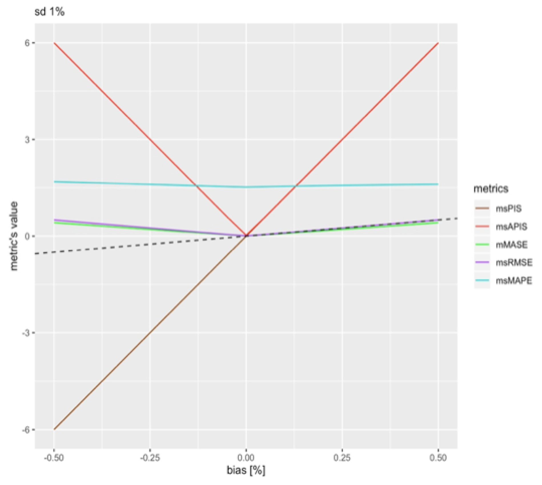
Let us evaluate bias sensitivity by fixing the standard deviation of forecasting models to 1% and then varying the bias from $-50$% to $+50$% of the in-sample mean.

Figure 4 presents the variation of performance metrics for changes in bias of forecasts. Both cumulative metrics seem to be more sensitive to bias. $msRMSE$ and $mMASE$ are close to the real bias values as shown by the dashed line. The variation in the values of metrics is also partly linear. The slope of this linear trend will, therefore, be estimated in the same way as standard deviation sensitivity, but with an absolute value to remove the sign from the slope:

$$vr=mean\left(\frac{L(\mu +\mathsf{\Delta })-L\left(\mu \right)}{\mathsf{\Delta }}\right)$$

(17)

where $L\left(\mu \right)$ is the performance metric expressed in function of bias $\mu$ and $\mathsf{\Delta }$, the variation in bias, which is 5%.

Table 3. Average variation rate of performance metrics for a variation in bias and fixed standard deviation of forecast models.

Metric	msPIS	msAPIS	mMASE	msRMSE	msMAPE
variation rate (vr)	12.00	11.87	0.80	0.95	0.28

represents the average variation rate considering a symmetric rate. It brings a slight simplification to the result in the case of $msAPIS$ and $msMAPE$. The difference in the calculated rate is noticeable when comparing $msAPIS$ with $msPIS$, which does not have this effect around zero since the effect of standard deviation on msPIS is null, on average. Refs. [11,18] noted that $msMAPE$ provides higher penalties to a negative bias than for a positive bias. The difference in rates between the negative and positive bias for $msMAPE$ is around 0.11. Meaning that the variation rate is greater by 0.11 when bias is negative, versus when it is positive. All metrics have the same order of magnitude in $vr$ except for cumulative metrics, which are of two orders of magnitude higher. $msRMSE$ is the closest metric to real bias.

4.4. Standard Deviation-Bias Sensitivity

4.4.1. Standard Deviation in Function of Bias

For the first measurements of sensitivity, bias, and then standard deviation, were fixed to a minimal value. This contrasts with situations in real life, in which selection of models probably implies identifying models with different values of bias and standard deviation. This section will, therefore, study the $vr$ of performance metrics for a change of both standard deviation and bias.

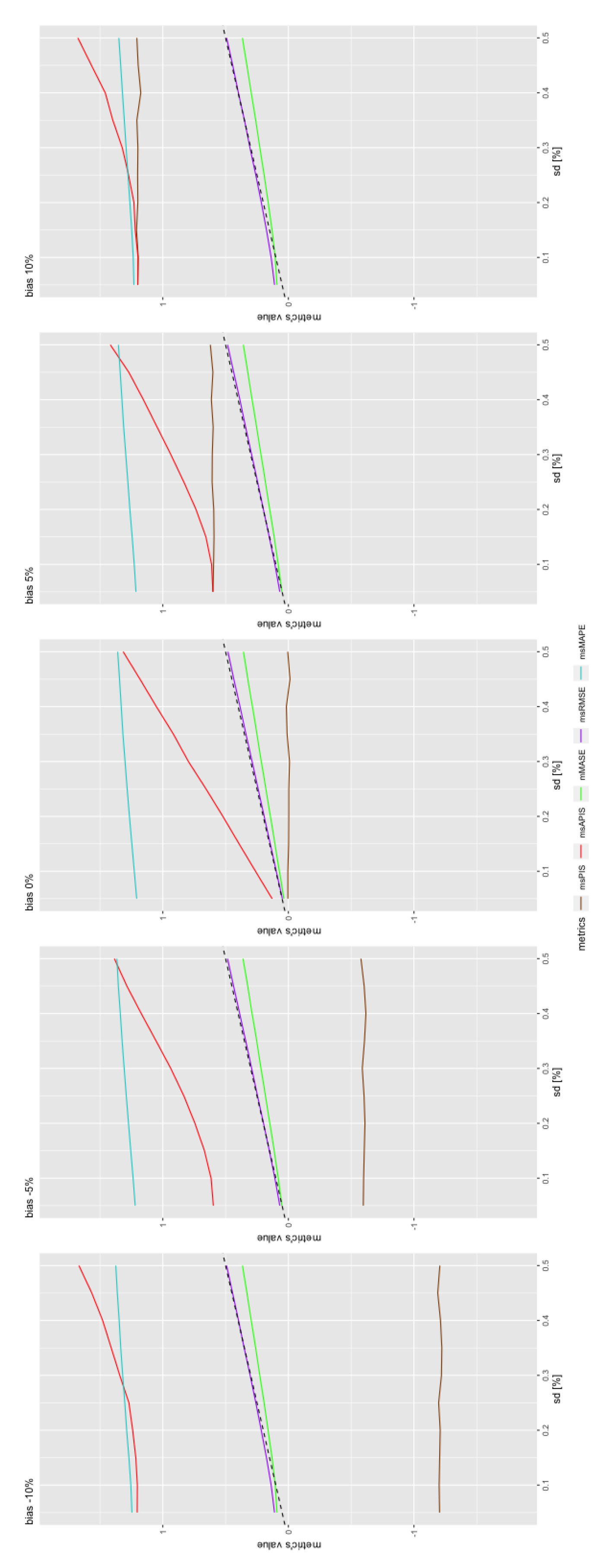
Figure 5 shows the metric’s value ($vr$) in function of a model’s standard deviation for different values of bias. The growth in all is linear, except for $msAPIS$, which has two modes. The first mode makes $msAPIS$ behave like $msPIS$. It is the case until standard deviation reaches a high enough value so that an increase in standard deviation has an impact on the metrics value. All other metrics also present two modes, but with the flat mode being much shorter. The difference between the length of the first mode is explained by the variation rate of bias, which is greater for $msAPIS$ than for the other metrics, which have similar variation rates for both standard deviation and bias. $msPIS$ converges to values close to bias and it is not affected by standard deviation. To represent the impact of bias on the standard deviation $vr$, its variation is plotted for every bias value. To do so, the average $vr$ in standard deviation direction of the different metrics is taken.

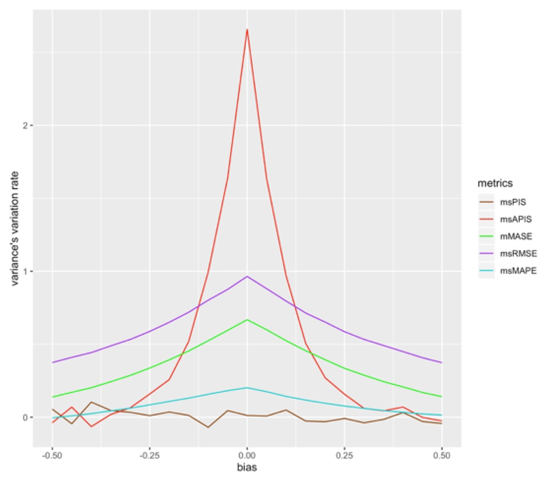
Figure 6 shows the variation rate of standard deviation when the bias is changed. $msAPIS$ is strongly influenced by a change in bias and the variation rate in the standard deviation direction goes to values close to zero for high absolute values of bias.

These results allow to conclude that the most sensitive metric to standard deviation would be $msRMSE$ in the presence of high bias. $msAPIS$ is the most sensitive metric to standard deviation in cases in which the absolute bias is less than 5% of the in-sample mean. It is also the least stable metric to variation of standard deviation in the presence of high bias. $msMAPE$ is the least sensitive metric, which has a variation rate close to zero for any bias value. $msPIS$ is not affected by standard deviation since averaging the different series errors cancels the negative and positive errors.

4.4.2. Bias in Function of Standard Deviation

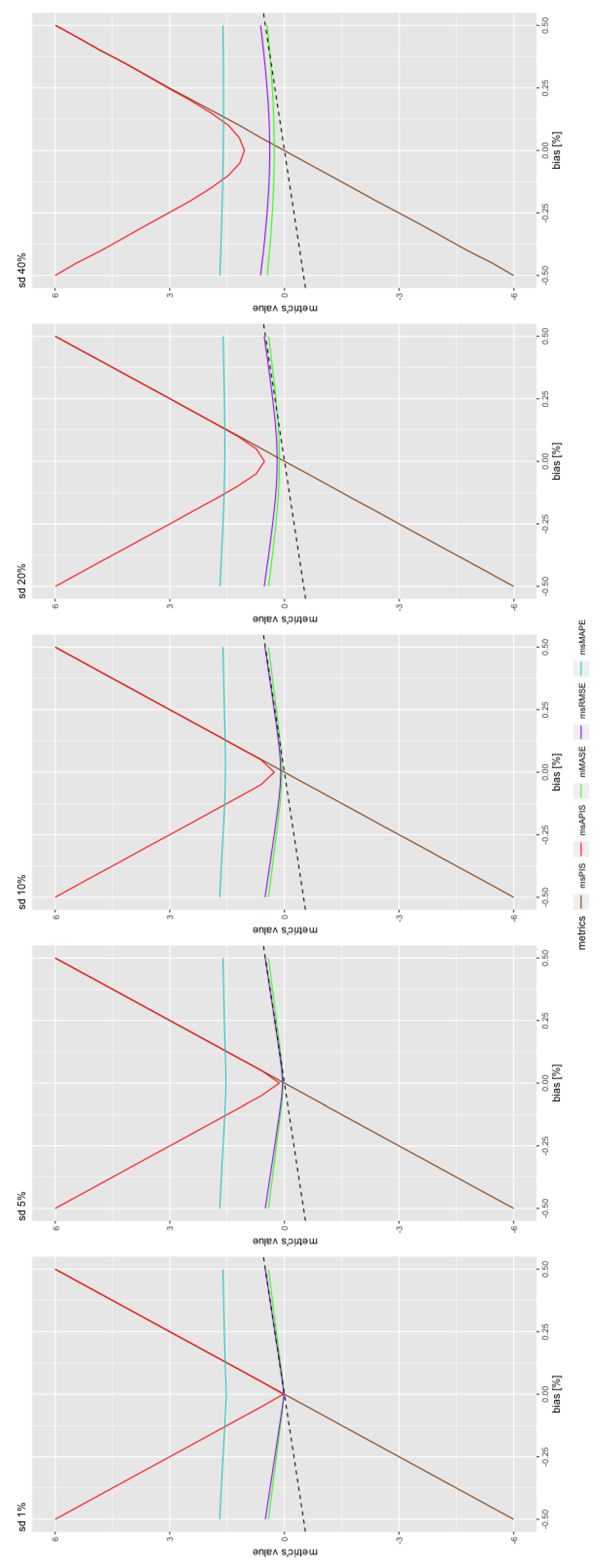
The same process applied in Section 4.4.1 can be applied with the bias in function of standard deviation. Figure 7 shows the impact of a change in standard deviation on the shape of the metric’s value in function of bias. Here, the variation rate change around the null bias. This is the case for all series, but the effect is more pronounced for $msAPIS$. Indeed, the variation seems to flatten and the flattening seems to increase with the standard deviation. This could be explained by the fact that a higher standard deviation means a higher metric value. So, the origin in the case of null bias is higher in the presence of high standard deviation, and a small increase in the bias is insignificant compared to the standard deviation.

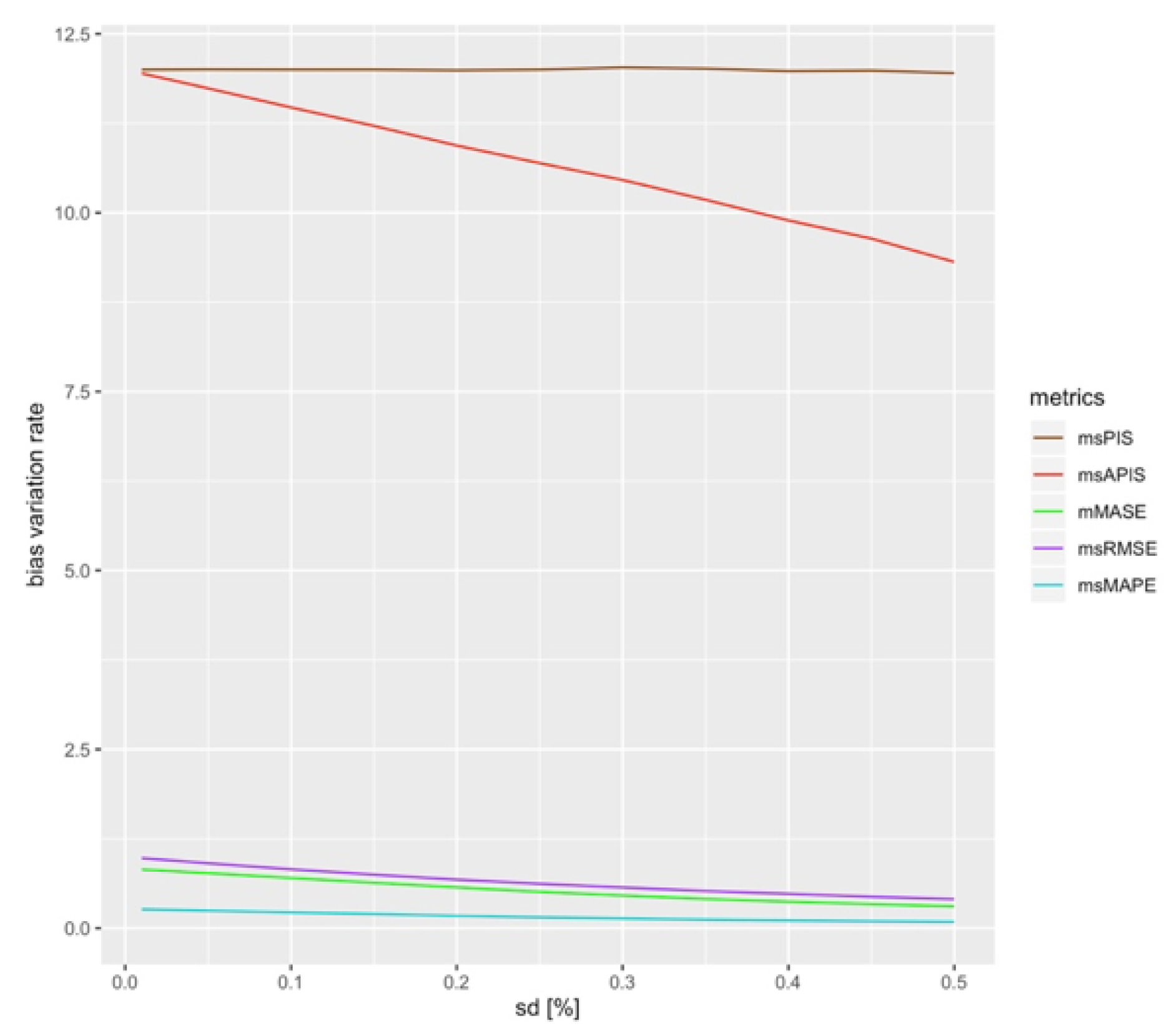
Figure 8 presents the variation rate of the bias when the standard deviation is changed. $msAPIS$ is the second most sensitive metric after $msPIS$, which is constant for all standard deviation values. All the other ones are close together, with $msRMSE$ slightly more sensitive than the others and $msMAPE$ is the least sensitive metric after $msPIS$.

4.5. Reliability of the Metrics

For every configuration, reliability has been measured in function of the number of series averaged performance and the number of forecast horizons. To simplify visualization, only extreme values of forecast horizons were kept: $h=1$ and $h=23$. The + and – configurations, as presented in Table 1, were set to be of one order of magnitude different. The different values used are presented in

Table 4. Values of each parameter for all of the different configurations.

Cases	$\mathit{\mu }$		$\mathit{\sigma }$		$\mathbf{\Delta }\mathbf{\sigma }$		$\mathbf{\Delta }\mathit{\mu }$
	+	−	+	−	+	−	+	−
Fixed Bias	2%	0.1%	1%	0.01%	0.1%	0.01%	0
Fixed Standard Deviation	1%	0.01%	2%	0.1%	0		0.1%	0.01%

. In each configuration, 25 different models were trained with a difference of $\mathsf{\Delta }\sigma$ or $\mathsf{\Delta }\mu$ for their error distribution parameter.

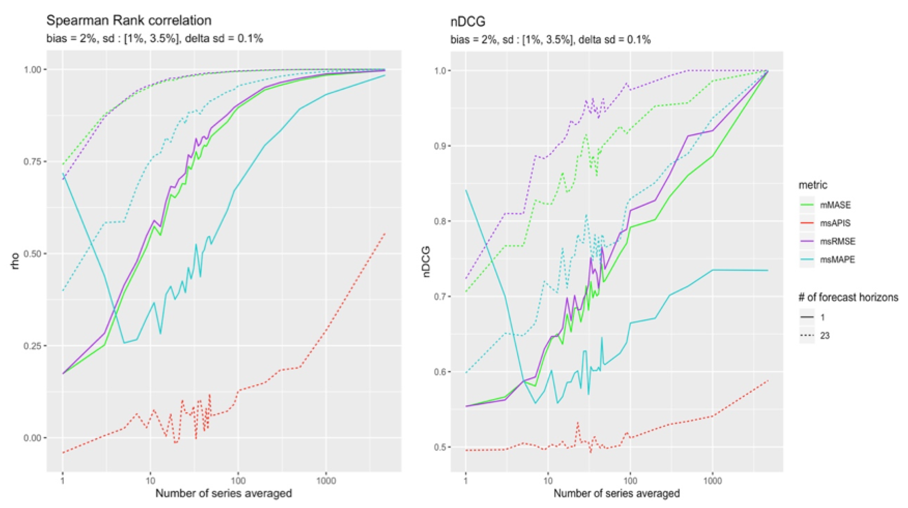
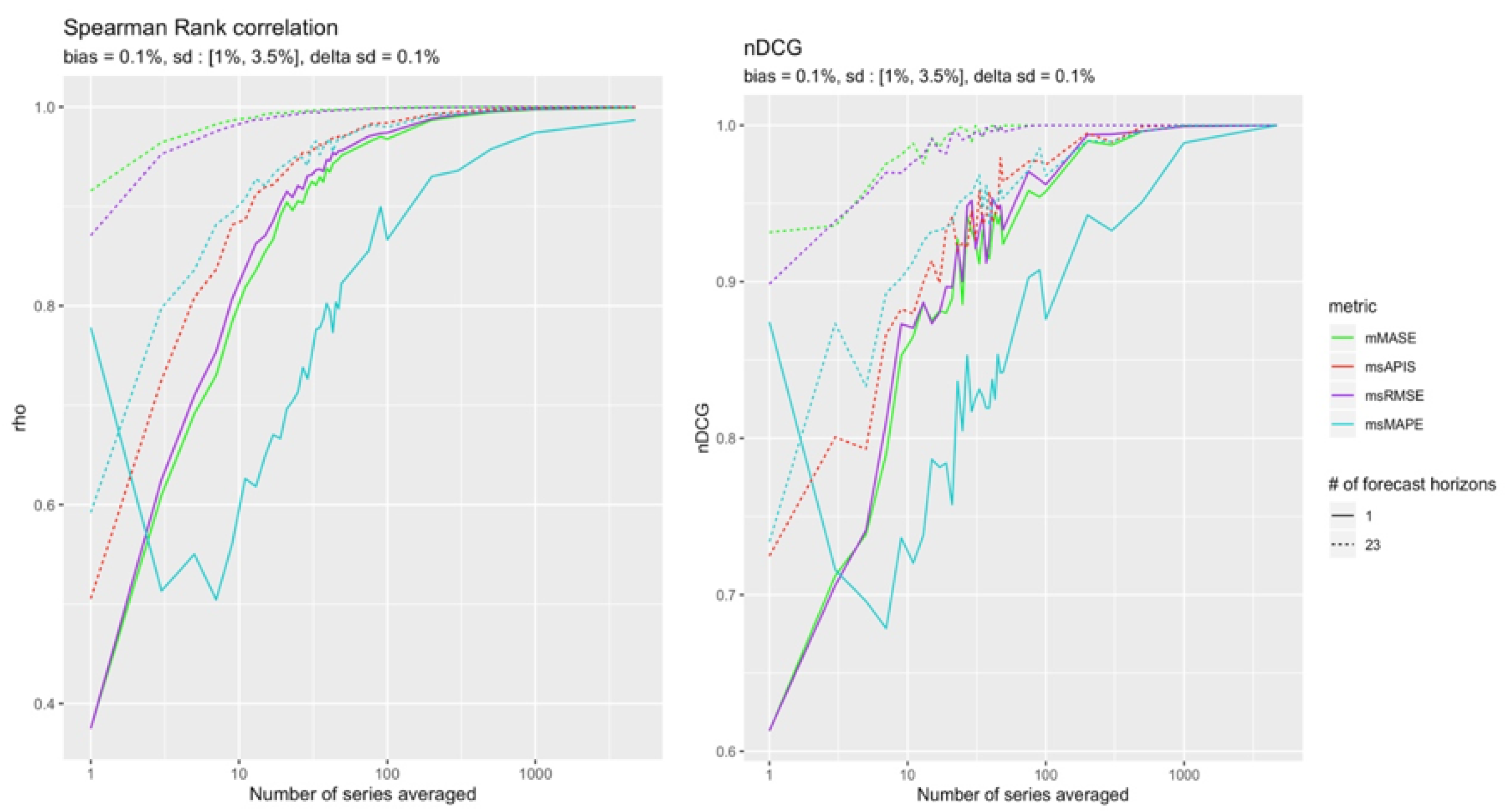
4.5.1. Reliability to a Change in Standard Deviation

Three different cases can be distinguished when changing the standard deviation of the models. The first case is the one with all the models of the same order of magnitude so $\sigma$, $\mu$ and $\mathsf{\Delta }\sigma$ in − or + configuration. The second is when the bias is of a high magnitude and the third is when the bias has a small order of magnitude. Since $msPIS$ is invariant to standard deviation, it was removed from the following figures.

Same Order of Magnitude

The Figure 9 and Figure 10 present Spearman’s rank correlation and nDCG in function of the number of series performance averaged. The two different types of lines present the number of forecast horizons used. The solid line presents the case in which a single point forecast is evaluated. The dashed line is for cases with 23 forecast horizons.

Figure 9 and Figure 10 both show the superiority of msRMSE in ranking the models in the correct order. Even though the correlation of mMASE and msRMSE show that their rankings are both going in the same direction as the real ranking, nDCG clearly distinguishes both metrics, with msRMSE converging more quickly to a perfect ranking. sMAPE presents some interesting properties that will be discussed in Section 5.

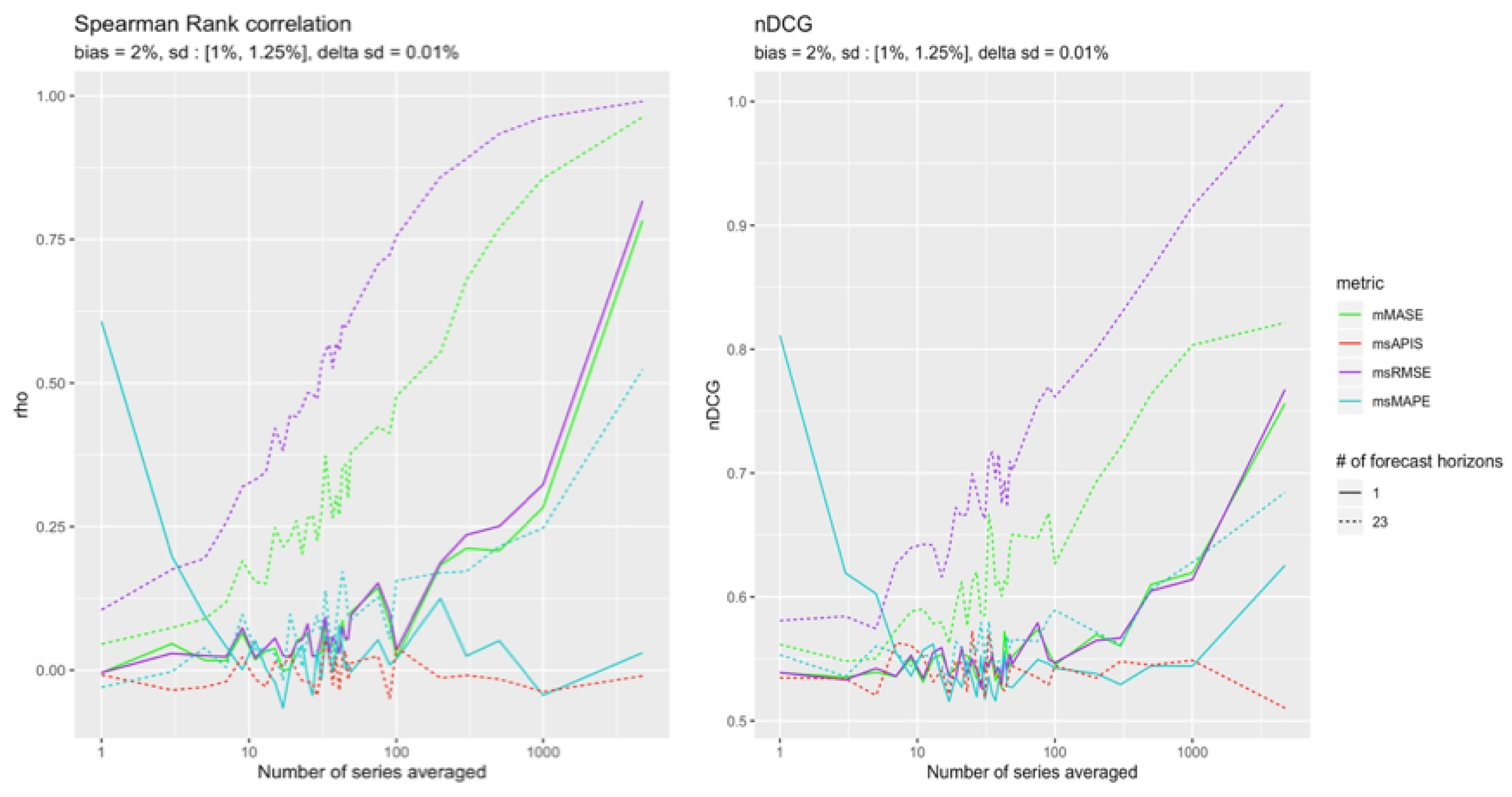
High Bias

Results in Figure 11 correspond to what was found in Section 4.4.1 where most metric sensitivity to standard deviation decreased in the presence of a high bias. The least impacted metrics by bias were $msRMSE$ and $mMASE$. Figure 6 also shows that $msRMSE$ was slightly more sensitive to standard deviation in presence of a high bias than $mMASE$. This trend might increase when increasing the difference between the two parameters. This could explain the results of Figure 12.

This section presents the results for a configuration with a high (+) bias. Figure 12 shows that in the presence of high bias compared to standard deviation, no metric can detect changes in standard deviation no matter how many observations are used, except for $msRMSE$. In both configurations, $msRMSE$ is the most reliable metric.

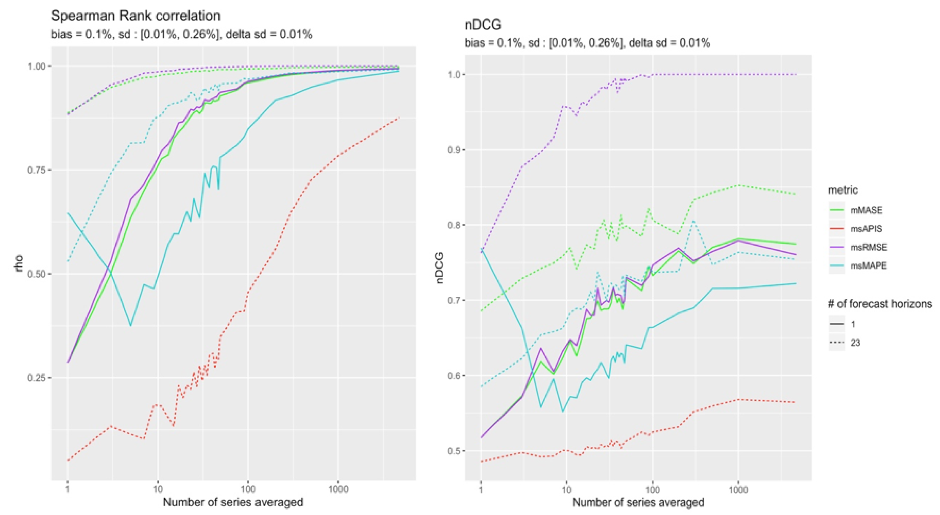
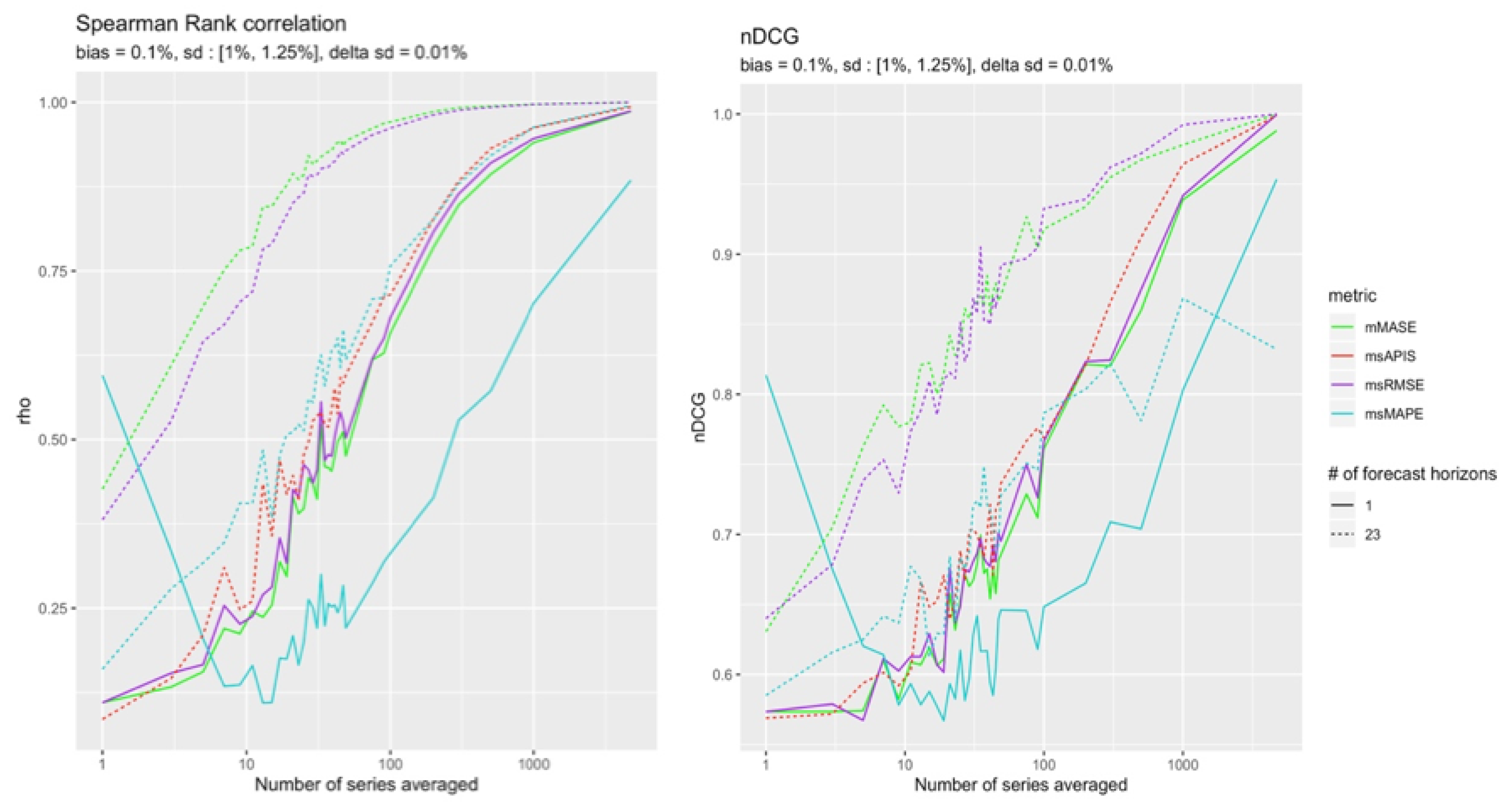
Small Bias

The remaining cases are those in which a bias is in a (−) configuration. The Figure 13 and Figure 14 show which metric performs better in the quasi-absence of bias. Although the results are tighter, it is still possible to distinguish slightly more reliable results from $mMASE$ in the presence of 23 forecast points. $msRMSE$ is slightly more reliable for a single point forecast.

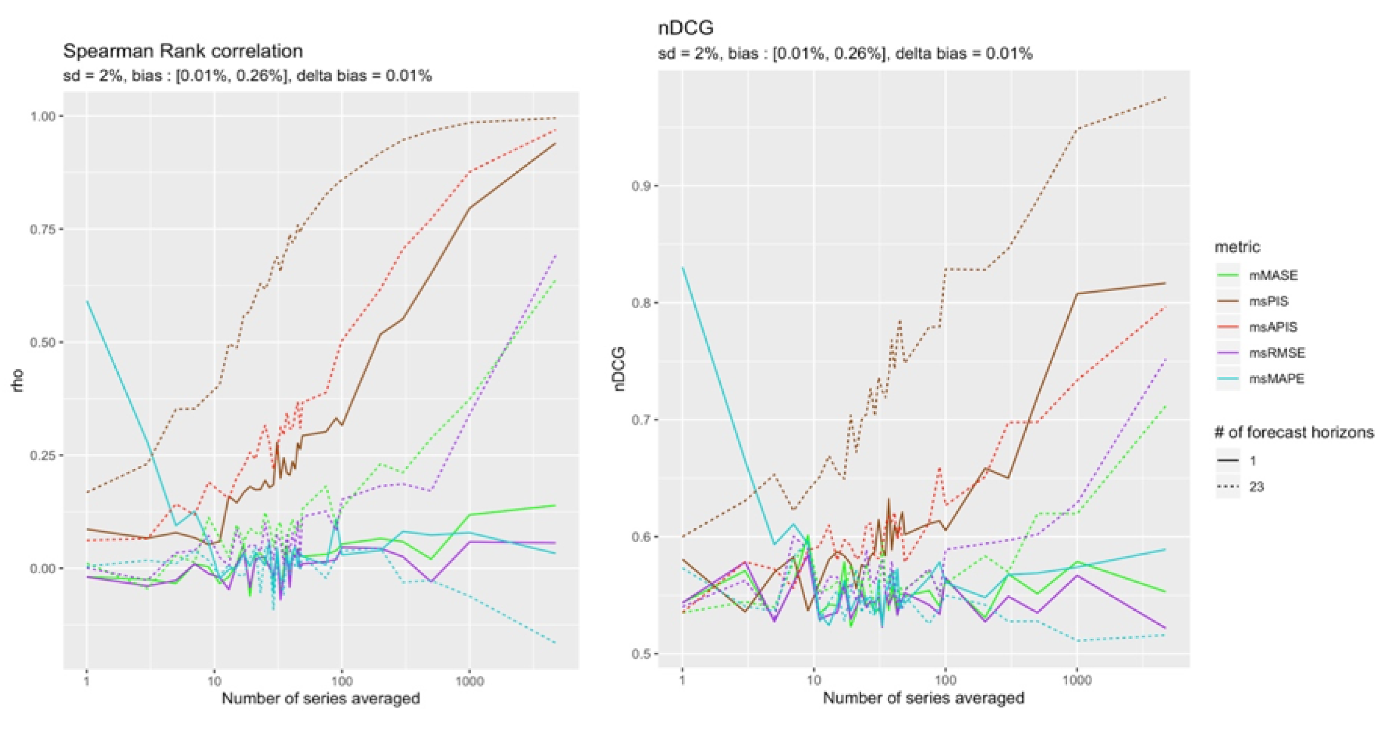
4.5.2. Reliability to Change in Bias

When it comes to detecting change in bias, three cases can be distinguished. The first one is configurations with high standard deviation and high bias. The second one is high standard deviation and small bias. The third one is cases with small standard deviation configurations.

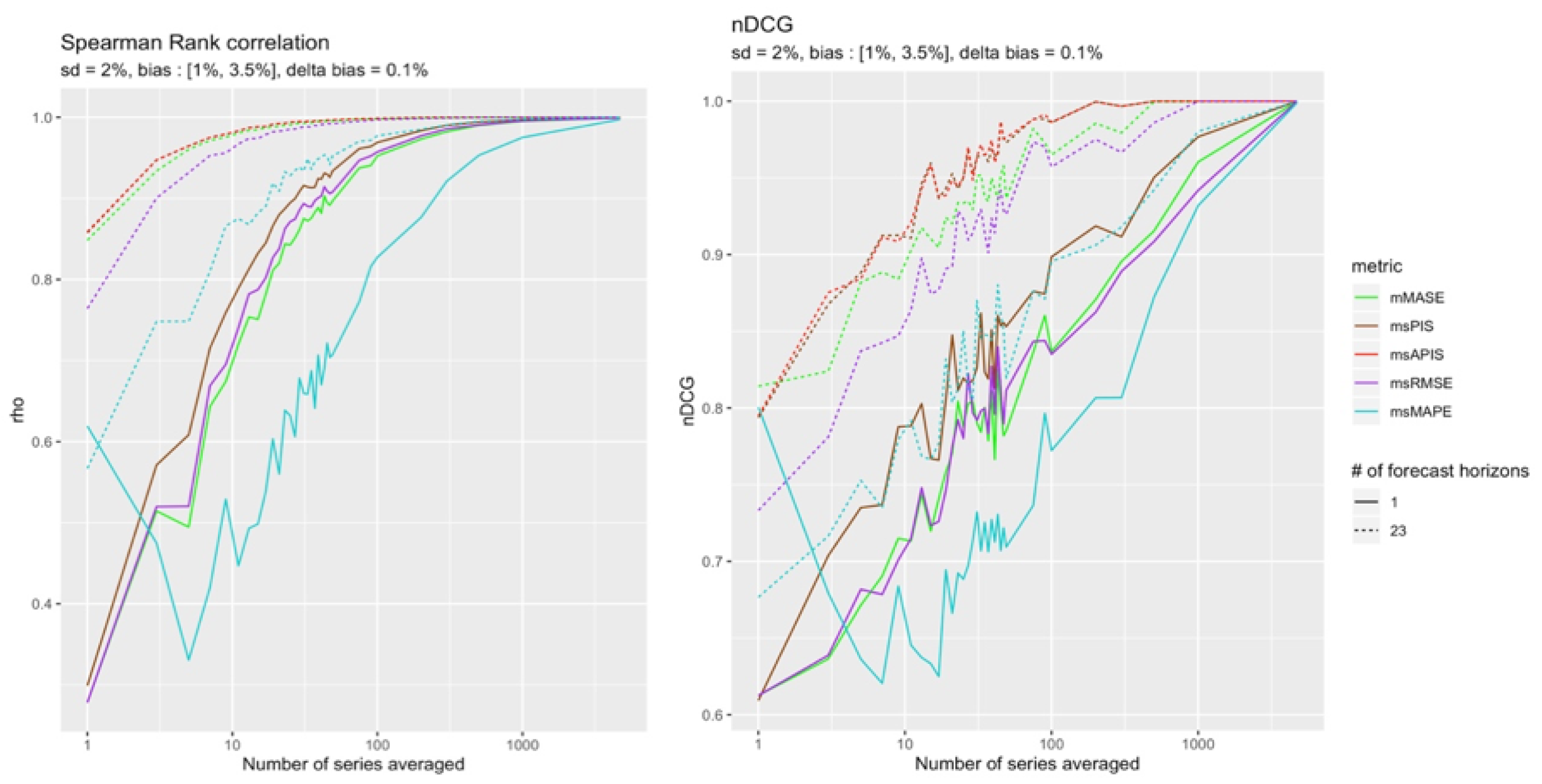
High Standard Deviation and High Bias

The two cases with high standard deviation and high bias are presented in the Figure 15 and Figure 16.

As expected, the cumulative metrics $msPIS$ and $msAPIS$ were more reliable than the others in detecting bias. However, $mMASE$ and $msRMSE$ were both able to reach a perfect ranking with all the available observations.

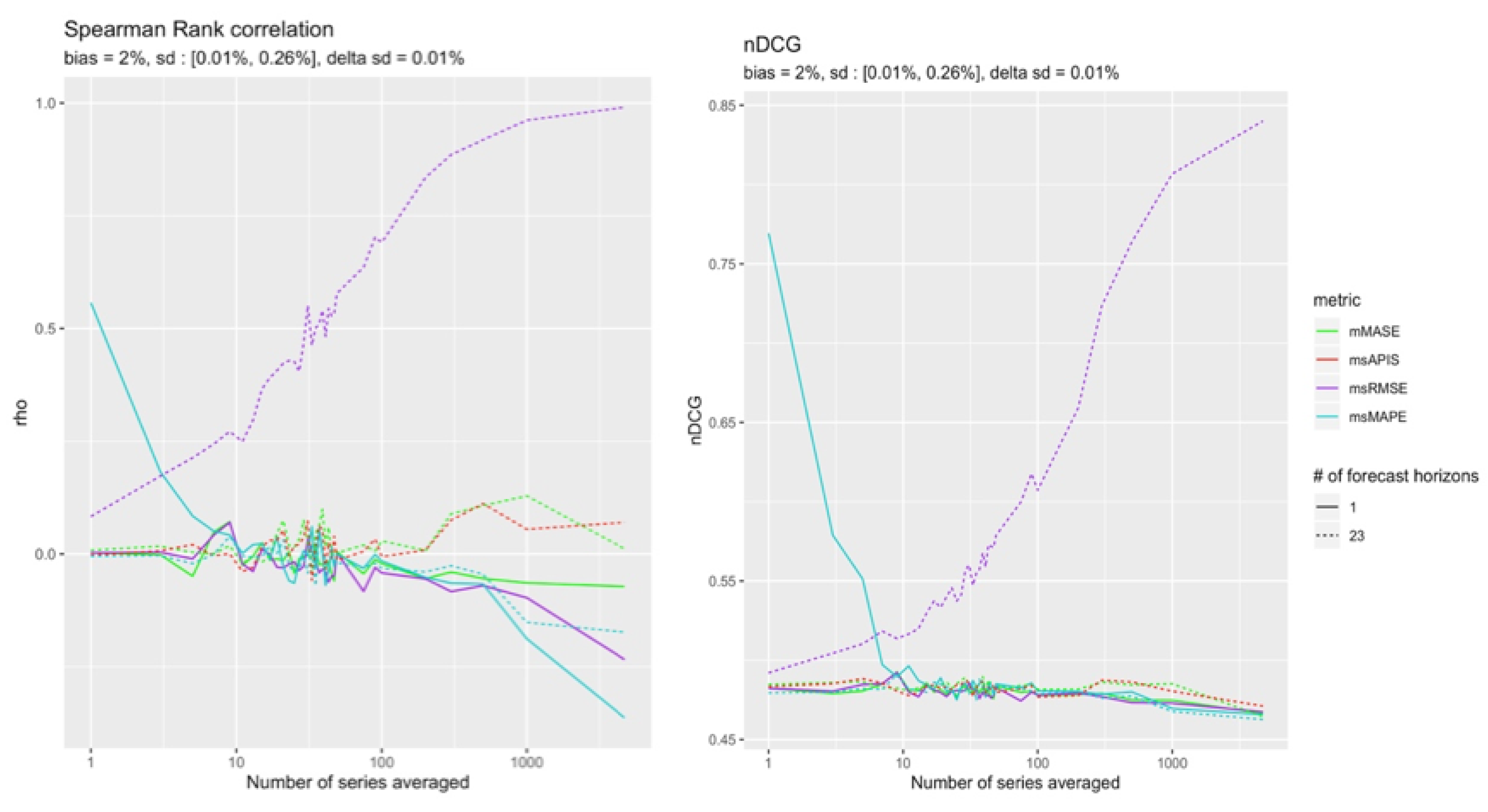
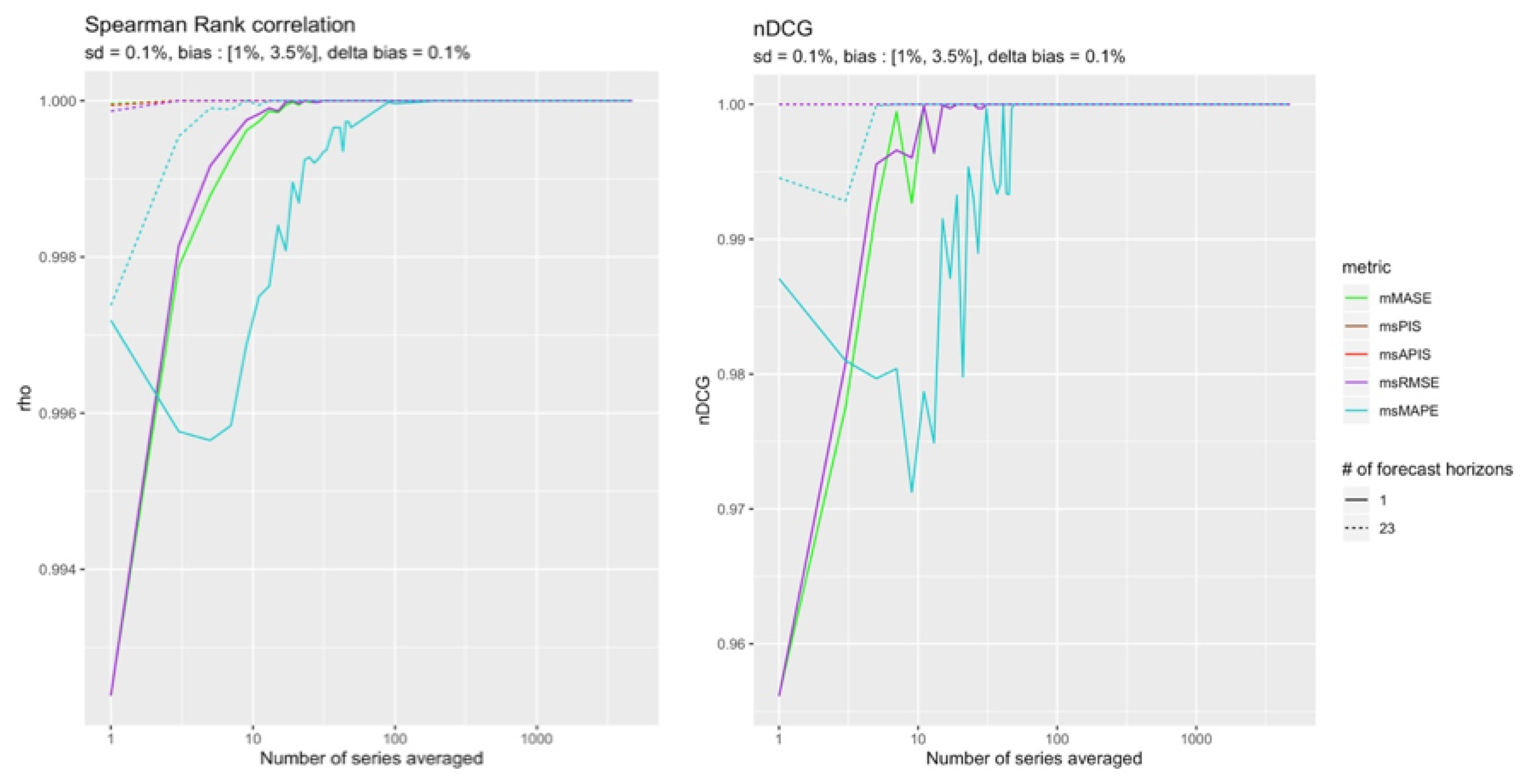
High Standard Deviation and Low Bias

This configuration is the only one for which $msPIS$ was the only metric able to converge to a perfect ranking (see Figure 17).

This result confirms what was found in Section 4.4.2, where in the presence of high standard deviation, the sensitivity of most metrics to bias decreases to nearly zero.

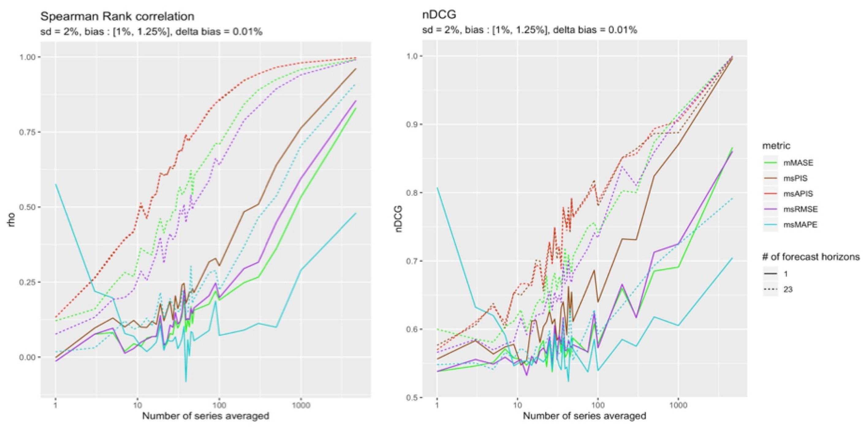
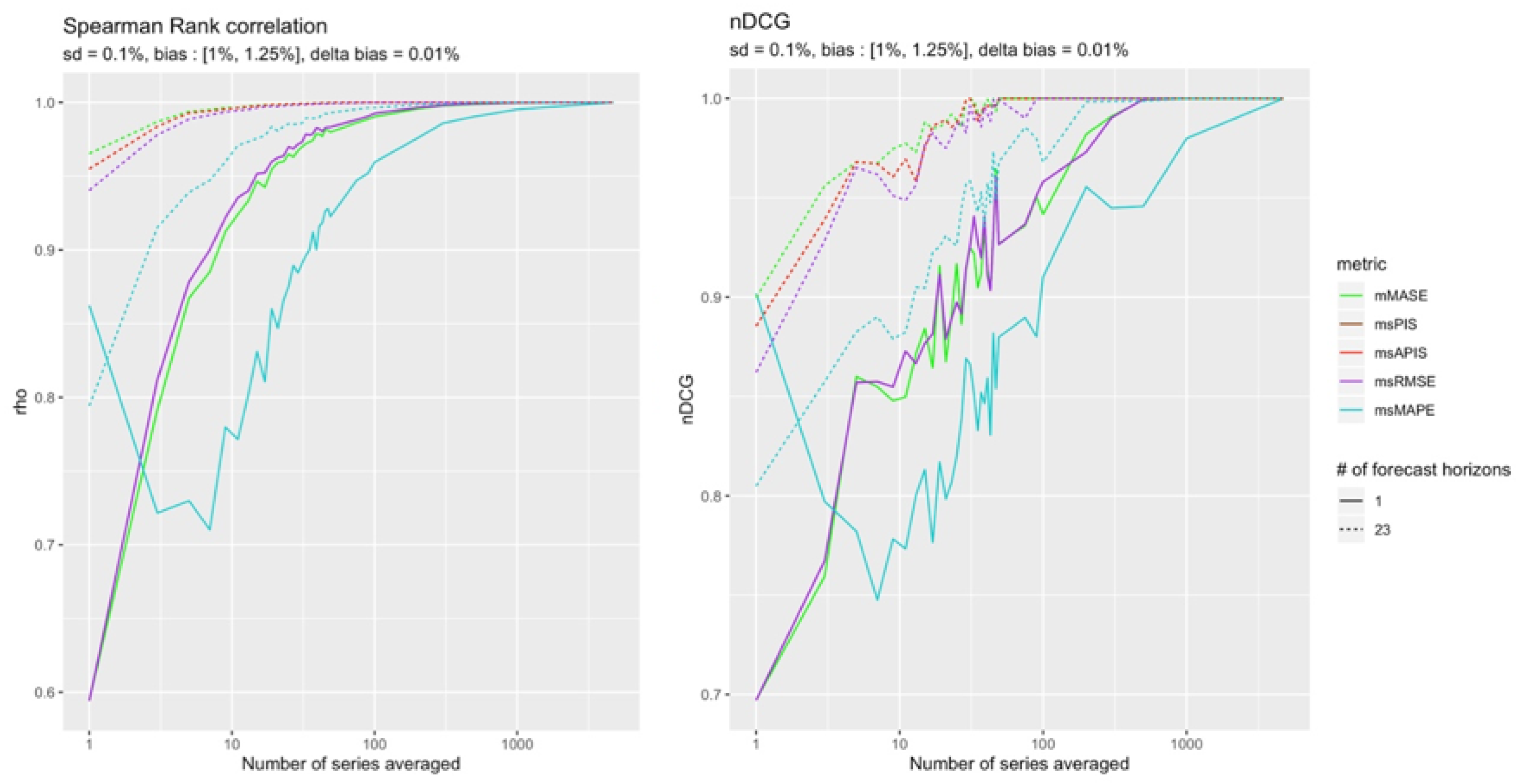
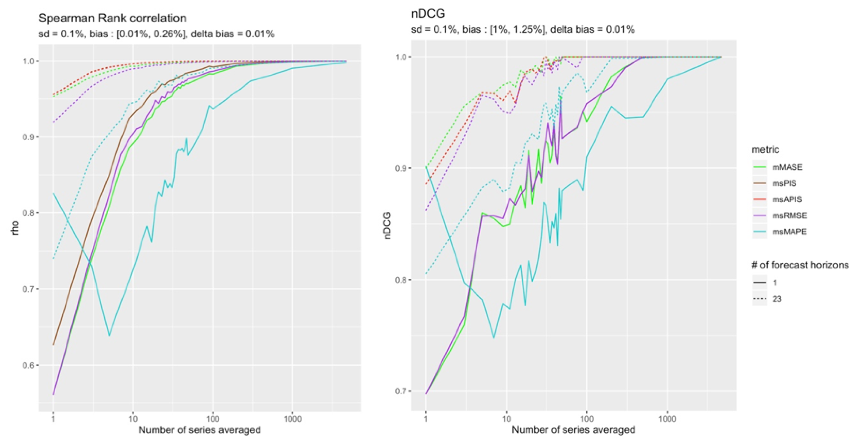
Small Standard Deviation

The final case where standard deviation is in (−) configuration also corroborates with the results in Section 4.4.2.

It has been shown that when standard deviation is small, all metrics have a non-null variation rate for bias. This is what the Figure 18, Figure 19 and Figure 20 present.

Indeed, no metric’s variation rate for bias is null for small values of standard deviation, but metrics with the most important sensitivity to bias are not superior to the other metrics. This result was found in other cases, such as those in Section 4.5.1, in which $msAPIS$ did not perform as well as expected based on the sensitivity results (Figure 6). The next section will discuss this and will study further results of a single point forecast for a single series to try to explain the $msMAPE$ results.

5. Result Analysis

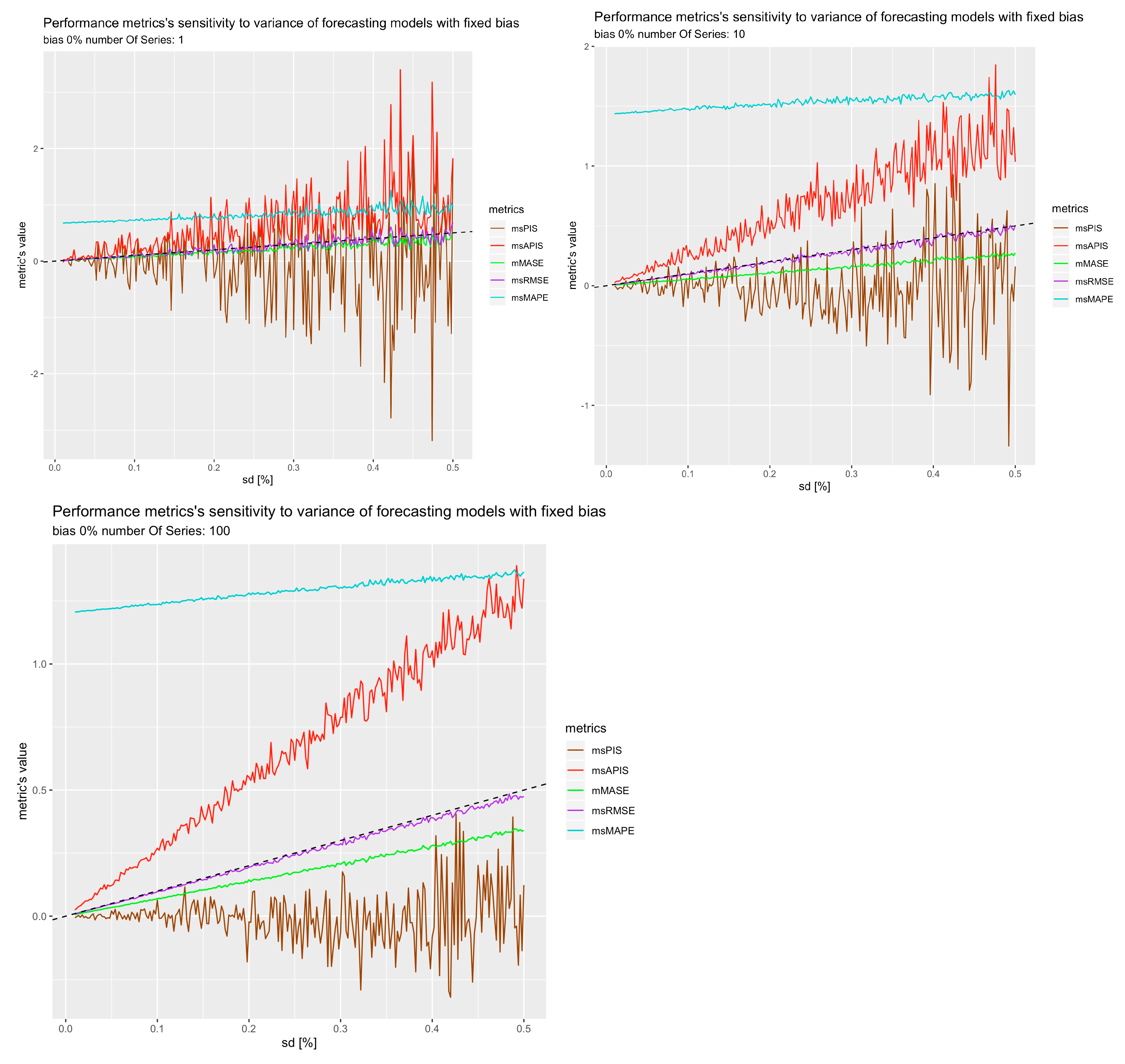
Following the reliability results, one would conclude that sensitivity did not have much impact on reliability. However, to measure sensitivity, all 23 forecasts horizons were used with all series. If the sensitivity experiment is rerun with 1, 10, and 100 series instead of thousands, it is possible to see how the amount of series affects sensitivity and reliability (Figure 21), which explains reliability results.

From the Figure 21, the observation is that the cumulative metrics are the most affected by the number of series used to average results. That makes sense with previous reliability results, in which the increase in reliability for $msAPIS$ could only be observed for a high number of averaged series performances. To further study the results of $msMAPE$ for a single series and a point forecast, the level of intermittence allowed in the horizon periods varied to see whether the proportion of zeros in the horizon periods impact the reliability of $msMAPE$. 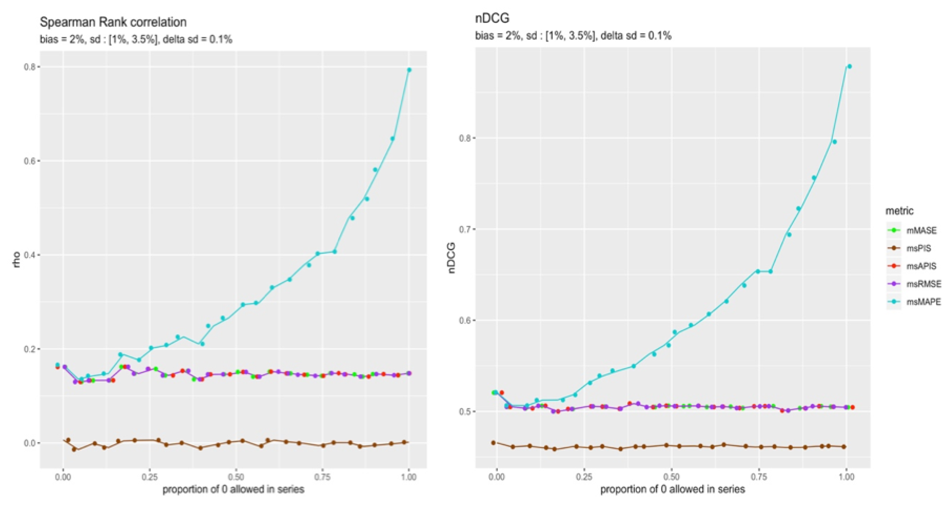Figure 22 shows the reliability of all metrics when the allowable proportion of zeros is less than a threshold. So, when the proportion of 0 allowed in a series is 0, it means that only the series with no zero demand within their horizon periods were kept. On the other hand, if the proportion of 0 demand allowed is 1, it means all series were kept. The average results of all the single series respecting the threshold are represented in the Figure 22.

There seems to be a relationship between the reliability of $msMAPE$ for a single time series point forecast and the level of intermittence in the series. This is probably caused by the fact that near zero demand $msMAPE$ can explode to infinity, making its sensitivity to small errors greater. Finally,

Table 5. Best choice of metric for different cases based on the reliability results.

	Number of Series
Point Forecast	1		<1000		>1000
	$\mathbf{\sigma }$	$\mathsf{\mu }$	$\mathbf{\sigma }$	$\mathsf{\mu }$	$\mathbf{\sigma }$	$\mathsf{\mu }$
Single	$msMAPE$	$msMAPE$	$msRMSE$	$msPIS$	$MASE$/$msRMSE$	$msPIS$
Multiple	$msRMSE$	$msPIS$	$msRMSE$	$msPIS$	$msRMSE$	$msPIS$

summarizes the results of Section 4.5.

In the case of a single time series point forecast, the conclusions in Table 5 only hold in the presence of a series with a high level of intermittent demand. Other results show that the best performance metrics are $msPIS$ to detect bias and $msRMSE$ to detect standard deviation. So, to detect both the bias and the standard deviation, one must first select models of the same order of magnitude according to the absolute value of $msPIS$. This ensures to keep the models of minimal bias without consideration to standard deviation. Next, the selected models need to be ranked according to $msRMSE$. This strategy ensures that the models of minimal bias are kept, and then ranked according to their standard deviation.

6. Conclusions

The goal of this paper was to present a new methodology to assess the precision and reliability of performance metrics. Fictitious forecasting models were defined as the addition of a noise of a known distribution to the actual values of the series. Given that the error distribution of the models was known, it was possible to estimate the sensitivity of metrics to changes in bias and standard deviation of the fictitious models. It was also possible to rank the models based on their error distribution, allowing the reliability of performance metrics to be studied in different cases. It is to the best of our knowledge a first attempt at quantifying the sensitivity of performance metrics. Sensitivity is highly influenced by the number of points used to average the performance. Results have shown that, with thousands of points for the average, $msAPIS$ was the most sensitive metric in most cases, followed by $msRMSE$ and $mMASE$, while the least sensitive metric was $msMAPE$. This result contrasts with previous beliefs that $MASE$ should be preferred because of its mathematical properties. The reliability results showed that, in most cases, $msRMSE$ was the most reliable metric, followed by $mMASE$. The exception is for cases where the models’ differences were due to a change in bias. In those cases, cumulative metrics, such as $msPIS$ and $msAPIS$, were more reliable. A surprising result was the ability of $msMAPE$ to rank single point forecasting models for a single time series with much more reliability than the other metrics. This result is related to the level of intermittence of the time series. Removing intermittent time series with a high proportion of zeros from the dataset brings the reliability of $msMAPE$ closer to other metrics’ reliability.

Thus, the results offer a new perspective on performance metrics, where the proposed methodology has allowed to figure some metrics were more reliable to changes in bias or in variance. Therefore, we propose a strategy to select the best forecasting model by first selecting models with the same order of magnitude of the absolute value of $msPIS$ and then ranking the selected models based on $msRMSE$.

In the present study, the error was defined has the distance between the predicted and real values. If the error would be defined on a different basis, a percentage of the real value for example, our conclusions may not apply, and supplementary work must be done.

Future work could study nDCG with relevance in function of both bias and standard deviation to verify how much more reliable selection techniques are when using this last strategy in comparison to mean rank methods.