Evaluating the Comparative Accuracy of COVID-19 Mortality Forecasts: An Analysis of the First-Wave Mortality Forecasts in the United States

Abstract

The sudden onset of the COVID-19 pandemic posed significant challenges for forecasting professionals worldwide. This article examines the early forecasts of COVID-19 transmission, using the context of the United States, one of the early epicenters of the crisis. The article compares the relative accuracy of selected models from two forecasters who informed government policy in the first three months of the pandemic, the Institute of Health Metrics and Evaluation (IHME) and Columbia University. Furthermore, we examine whether the forecasts improved as more data became available in the subsequent months of the pandemic, using the forecasts from Los Alamos National Laboratory and the University of Texas, Austin. The analysis focuses on mortality estimates and compares forecasts using epidemiological and curve-fitting models during the first wave of the pandemic from March 2020 to October 2020. As health agencies worldwide struggled with uncertainty in models and projections of COVID-19 caseload and mortality, this article provides important insights that can be useful for crafting policy responses to the ongoing pandemic and future outbreaks.

1. Introduction

The coronavirus pandemic has wreaked tremendous havoc worldwide, resulting in the loss of human lives and severe economic disruptions. The expansion of vaccines has reduced the mortality rates associated with the virus, but the pandemic is still far from over. In the early days of the pandemic in 2020, policymakers around the world scurried for containment measures and non-pharmaceutical interventions (NPIs)—including lockdowns, quarantine protocols, and social distancing. However, the uncertainty around virus transmission dominated the headlines, due to a wide range of forecasts put forth by researchers. On 16 March 2020, one of the models from the Imperial College, London, sent shockwaves across the United States, predicting 2.2 million deaths in the absence of spontaneous changes in individual behavior and control measures [1]. In hindsight, the model obviously had a significant error, but the counterfactual states could not be observed since stringent containment measures were, indeed, put in place. Furthermore, the vaccines arrived much earlier than anticipated in the outbreak’s initial months, changing the trajectory of early forecasts. Since then, dozens of national and international forecasts and projections have informed policy responses, including shutdowns and reopening guidelines. These models broadly fall under three major categories: mechanistic models (e.g., SEIR models), statistical time series and exponential smoothing models, and deep learning or machine learning models. In this article, we focus on the first two categories and examine the accuracy of these forecasts in the early days of a pandemic, when past data and patterns were limited.

We primarily rely on the forecasts of four major agencies that informed public policy decisions in a significant way in the United States: University of Washington’s Institute of Health Metrics and Evaluation (IHME); Los Alamos National Laboratory (LANL); Columbia University’s Mailman School of Public Health (MIPH); and University of Texas, Austin. All of these models had different estimation approaches, but the latter two were versions of SEIR (Susceptible–Exposed–Infectious–Recovered) models that accounted for social distancing parameters, and the former were statistical forecasts based on curve-fitting approaches, the LANL model was an exponential smoothing time series model and IHME was a hybrid model that combined mechanistic and time series approaches. The IHME and Columbia models were at the center of policymaking concerning shutdowns and other non-pharmaceutical interventions in the early weeks of the pandemic in the U.S., and the White House heavily relied on the IHME model [2]. Governor Andrew Cuomo of New York State, one of the earliest epicenters of the crisis, compared forecasts for these agencies, and they informed policy choices regarding testing, purchase of medical equipment, and social distancing guidelines [3].

The actual number of cases remains unknown, due to the asymptomatic nature of COVID-19 for a large proportion of cases, lack of access to testing in the early days, and issues related to the voluntary choice of not taking the test under mild symptoms. In this context, for this analysis, we used only the number of deaths, The mortality estimates may also be biased, because reliable excess death estimates are not available, but the bias is relatively much smaller. In some states, the official estimates have been updated to include the excess deaths, reducing the potential for bias in the calculated forecast deviations. We compare the mortality forecasts to the actual number of deaths, as reported by the data tracker, moderated by the Center for Systems Science and Engineering (CSSE) at the John Hopkins University. The first six months of the pandemic were unique as the past data was unavailable, but the forecasters had more tools to work with as more information became available. On the other hand, the emergence of vaccines and new variants towards the end of 2020 posed new challenges for forecasting the trajectory of the pandemic. Due to these reasons, we focused on the first six months of the pandemic, from mid-March through early October to examine the efficiency of models in the early days of the pandemic. In the United States, the cases started to increase again in mid-October 2020, which was the beginning of the second wave that lasted through February 2021 and peaked in January 2021.

The rest of the article is organized into four sections. The next section briefly reviews available studies on COVID-19-related forecasts and highlights the practice and utility of forecast evaluation and comparisons across several disciplines. Section 3 summarizes the data and measures used in this paper, including a brief discussion on the advantages and disadvantages of different measures. Section 4 outlines the results and discusses its implications for forecasting the current pandemic and such events in the future. The last section discusses the limitations of the study and concludes.

2. Previous Research

A vast literature in forecasting focuses on the accuracy of forecasts and its underlying determinants [4,5]. Besides this, the practice of comparing multiple forecasts and examining variation by forecaster characteristics is also a well-established tradition, and can be found in various domains, particularly within the disciplines of business, economics, and finance [5,6,7,8]. Evaluation of forecasting models is also an increasing focus of short-term disease forecasting and recent studies have focused on infectious diseases, such as influenza and dengue [9,10,11]. The nature of the coronavirus pandemic and its timeline has posed unprecedented challenges that many forecasters and forecasting models were not prepared to account for, at least in the initial months. First, understanding how the virus spread, how long it sustained itself in different environments, and the transmission rate was very limited. Second, any significant precedence on social distancing outcomes and the general population’s compliance with shutdowns was not available, so uncertainty was inevitable. The forecasting models now have relatively much more information and robust assumptions than they had access to in the initial months of the coronavirus outbreak.

Table 1. Selected COVID-19 Forecasts, Methodology, Assumptions.

No.	Models	Method	Assumptions	Webpage
1.	Institute of Health Metrics and Evaluation (IHME)	Combination of Mechanistic transmission model and curve-fitting approach	Adjusted to differences in mobility.	https://covid19.healthdata.org/united-states-of-america
2.	Columbia University	Metapopulation SEIR model	Accounts for social distancing.	https://columbia.maps.arcgis.com/apps/webappviewer/index.html?id=ade6ba85450c4325a12a5b9c09ba796c
3.	Auquan Data Science	SEIR Model	No assumption about interventions.	https://covid19-infection-model.auquan.com/
4.	COVID-19 Simulator Consortium	SEIR Model	20% increase in contact rates after lifting statistics at home orders.	https://www.covid19sim.org/team
5.	Georgia Technology Authority	Deep Learning	Assumes effects of interventions embedded in the data.	https://www.cc.gatech.edu/~badityap/covid.html
6.	Imperial College, London	Ensembles of mechanistic transmission models	No specific assumptions about the interventions.	https://mrc-ide.github.io/covid19-short-term-forecasts/index.html
7.	John Hopkins University	Stochastic Metapopulation SEIR model	Assumes reduction in effectiveness of mitigation after lifting shelter-in-place.	https://github.com/HopkinsIDD/COVIDScenarioPipeline
8.	Los Alamos National Laboratory	Statistical dynamic growth model accounting for population susceptibility	Assumes the NPIs would continue.	https://covid-19.bsvgateway.org/
9.	Massachusetts Institute of Technology	SEIR Model	Assumes continuation of present interventions.	https://www.covidanalytics.io/projections
10.	Northeastern University	Metapopulation, age structured SLIR model	Assumes continuation of social distancing policies.	https://covid19.gleamproject.org/
11	Iowa State University	Nonparametric spatiotemporal model	No specific assumptions related to interventions.	http://www.covid19dashboard.us/
12	Predictive Science Inc.	Stochastic SEIRX model	Assumes that current interventions would not change.	https://github.com/predsci/DRAFT
13	US Army Engineer Research and Development Center	SEIR mechanistic model	Projections assume that interventions would not change.	https://www.cdc.gov/coronavirus/2019-ncov/covid-data/forecasting-us.html
14	University of California, Los Angeles	Modified SEIR Model	Projections assume that interventions would not change.	https://covid19.uclaml.org/
15	University of Texas, Austin	Nonlinear Bayesian hierarchical regression with a negative-binomial model	Estimate the extent of social distancing, using mobile phone geolocation data. Does not assume changes in social distancing during the forecast period.	https://covid-19.tacc.utexas.edu/projections/

summarizes the major forecasts for the United States that were being aggregated as part of the early ensemble forecasting efforts of the Center for Disease Control and Prevention (CDC). Some of these forecasts were epidemiological, and some were purely statistical forecasts, based on exponential smoothening and time series of observed trends.

The epidemiological projections relied on a variety of methods, including using simulations based on the behavior of earlier strains of the coronavirus family, like SARS-CoV-1 and MERS, using the transmission data from China, Italy, and Spain, and increasingly the information gained from the U.S. transmission behavior and social distancing compliance. Ref. [12] used a medical model of transmission behavior, based on the immunity, cross-immunity, and seasonality for Hcov-OC43 and HcoV-HKU1, to suggest that a seasonal resurgence is the most likely scenario, requiring intermittent social distancing through 2022 and resurgences as late as 2024. Another study used early data from Hubei province in China. between 11 January 2020 and 10 February 2020, and predicted that the cumulative case count in China by 29 February could reach 180,000 with a lower bound of 45,000 cases [13]. The official reality turned out to be much more optimistic than the one forecasted, perhaps owing to underreporting, effective non-pharmaceutical interventions, or flawed model assumptions. The epidemiological model by Imperial College, that was mentioned earlier, also deviated significantly because of the changes in underlying assumptions and global health response that ensued. The epidemiological models rely on various scientific assumptions related to the behavior of viruses, underlying health conditions and immunity, availability of health infrastructure, etc., which may pose a significant challenge for forecasting in the initial days of a new virus, such as COVID-19. However, as data becomes available, employing time series or purely statistical forecasting models could also be effective. For example, [14] used exponential smoothening with multiplicative error and multiplicative trend components to forecast the trajectory of COVID-19 outcomes. The forecasts released by [14] and their subsequent follow-up on social media, typically showed over-forecasting in cases and deaths, but the actual values were within the 50% prediction level, except in the first round [15]. Ref. [16] used local averaged time trend estimation that assumed no seasonality, and they argue that, in the short run, their forecasts outperformed the epidemiological forecasts, such as the ones from Imperial College. A probabilistic model from the Los Alamos National Laboratory in New Mexico compared the forecasts to the actuals and reported fairly robust coverage of the forecasts for three-week periods following their releases [17].

Though the statistical forecasts have immense appeal. since they can be created in real-time and can forecast micro-level patterns, for example, state or county-level trends, they have also come under criticism. Ref. [18] raised several concerns that warrant a careful approach toward statistical models in the case of epidemics. They highlighted that epidemic curves may not follow a normal distribution, and curves may fit early data in various ways, which may change as the epidemic progresses, for example, a second wave may occur and change things. They suggested that such models can be helpful for short-term predictions, but, otherwise, extreme caution has to be exercised, a point that is reaffirmed by [19]. They argued that, for long-term outcomes, only mechanistic models, like SEIR models, are reliable—many of the forecasts listed in Table 1 used SEIR models.

Some recent studies have examined the effectiveness of different models and also compared the individual models to ensemble forecasts. Ref. [20] evaluated the individual and ensemble forecasts and found that ensemble forecasts outperformed any individual forecasts, using the data from more than 90 different forecasting agencies at https://covid19forecasthub.org/ (last accessed: 10 September 2022). Ref. [21] evaluated the forecast accuracy of IHME data and found that IHME data underestimated mortality, and the results did not improve over time. Ref. [22] examined the efficacy of hybrid models against a range of technical forecasting models, using Italian Ministry of Health data, in early 2020, and found that hybrid models were better at capturing the pandemic’s linear, non-linear and seasonal patterns and significantly outperformed single time series models. Ref. [23] used the data from the second wave of the pandemic in India and the United States. They found that the ARIMA model had the best fit for India and the ARIMA-GRNN model had the best fit for the United States. Ref. [24] undertook an evaluation of thirteen forecasts for Germany and Poland during the ten weeks of the second wave and found considerable heterogeneity in both point estimates and the forecasts concerning spread. Ref. [25] argued that the COVID-19 pandemic highlighted the weakness of epidemic forecasting, and that when forecasts and forecast errors could determine the strength of policy measures, such as the implementation of lockdowns, they should receive closer scrutiny. This study adds to this growing literature and undertakes a comparative evaluation of two sets of statistical and epidemiological models, using trend-based comparison, and a set of forecast accuracy measures discussed in the next section. The findings have relevance for the practice of ensemble forecasting and the study of short-term forecasting of infectious diseases.

3. Materials and Methods

There are several challenges in comparing forecasts against actual outcomes. Agencies involved in forecasting often revise their estimates, and older forecasts disappear from the websites. The reporting formats of the forecasts often change, as do the assumptions underlying the forecasts. In this study, we focused on the forecasts of selected agencies and the information was collected as the forecasts became available from March to November 2020. The data was collected from four major sources:

■

Institute of Health Metrics and Evaluation (IHME), available at http://www.healthdata.org/covid/data-downloads, (last accessed: 10 September 2022)

■

Mailman Institute of Public Health at Columbia University (MIPH), available at https://github.com/shaman-lab/COVID-19Projection, (last accessed: 10 September 2022)

■

Los Alamos National Laboratory, available for download at https://covid-19.bsvgateway.org/, (last accessed: 10 September 2022)

■

University of Texas, Austin, available at https://covid-19.tacc.utexas.edu/dashboards/us/, (last accessed: 10 September 2022)

All forecasts evaluated were real-time ex post forecasts as made available by the Center for Systems Science and Engineering at John Hopkins University (CSSE) https://github.com/CSSEGISandData/COVID-19. Although both IHME and MIPH forecasted many data series and specified confidence intervals, for this analysis, only forecasts concerning the central tendency for mortality (death) were evaluated, due to the unreliability of caseload estimates in the early days of the pandemic. Mortality estimates have also come under scrutiny, as more information on excess mortality. due to COVID-19, has been documented (See, for example, efforts by the COVID-19 excess mortality collaborators published in the Lancet [26], 16–22 April 2022). MIPH produced numerous forecasts reflecting a variety of assumptions, and these assumptions have changed over time, and the MIPH data were simulations, assigning information to every county in the United States. These data were summarized into one nationwide forecast for each day.

The MIPH models considered hypothetical conditions labeled as follows to correspond to changes in social distancing and person-to-person contacts under stay-at-home orders: no intervention, 80 percent contacts, 70 percent contacts, and 60 percent contacts. For the United States, these data were detailed at the county level for each forecast day. For this analysis, the county-level details were aggregated to a value for the United States for each date. These were treated as four forecast categories, which were each evaluated: MIPH No intervention, MIPH 80, MIPH 70, and MIPH 60. However, they include substitute values for the March and May periods. In March, the categories were no intervention, 75 percent contacts, and 50 percent contacts. The 75 percent contacts was substituted for both MIPH 80 and MIPH 70, and the 50 percent contacts was substituted for MIPH 60. Beginning in May, the no intervention and 70 and 60 percent contacts were eliminated, and various other alternative 80 percent contacts were produced. For forecasts through to 7 May, a base level of 80 percent contacts was included, but, afterwards, only alternative values were shown. For as long as feasible the base level 80 percent contact was used for the Columbia 80 model. Afterwards the model, “w10p”, that commonly produced the largest number of deaths, was substituted. For MIPH 60 the base model, which had the lowest forecast of deaths, was used for the 3 May forecast, and, afterward, the model, “w5p”. which produced the least forecast of deaths, was used. For MIPH 70 the model, “1x”, which had an intermediate number of deaths, was used for the 3 May forecast, and, afterwards the model, “1x5p”, was used. The no intervention model consistently used the highest number of deaths, “w”, up to 3 May, and, afterwards, the model “w10p” Out of all these models, we highlighted the results of MIPH60 since that was closer to the actual social distancing during the period, as measured by Google’s Community Mobility reports [27].

The IHME model is relatively straightforward, showing only one central tendency forecast. Over the period of 25 March through 23 May there were 22 unique forecasts. After excluding observations up to and through the date of the forecast, the number of forecast periods ranged from 74 through 112. For the evaluated period, the observations ranged from 9 to 67, with an average of 44.

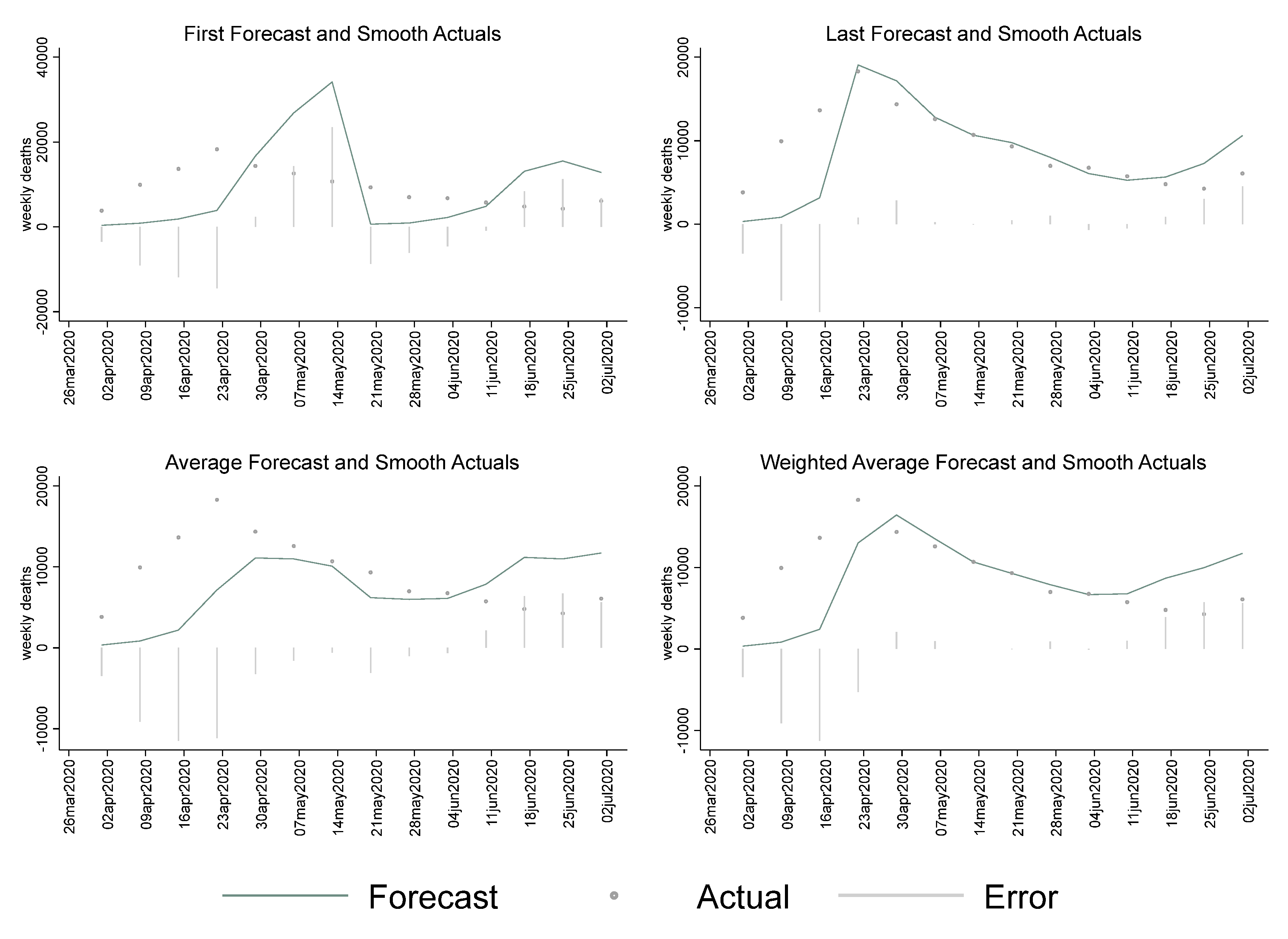
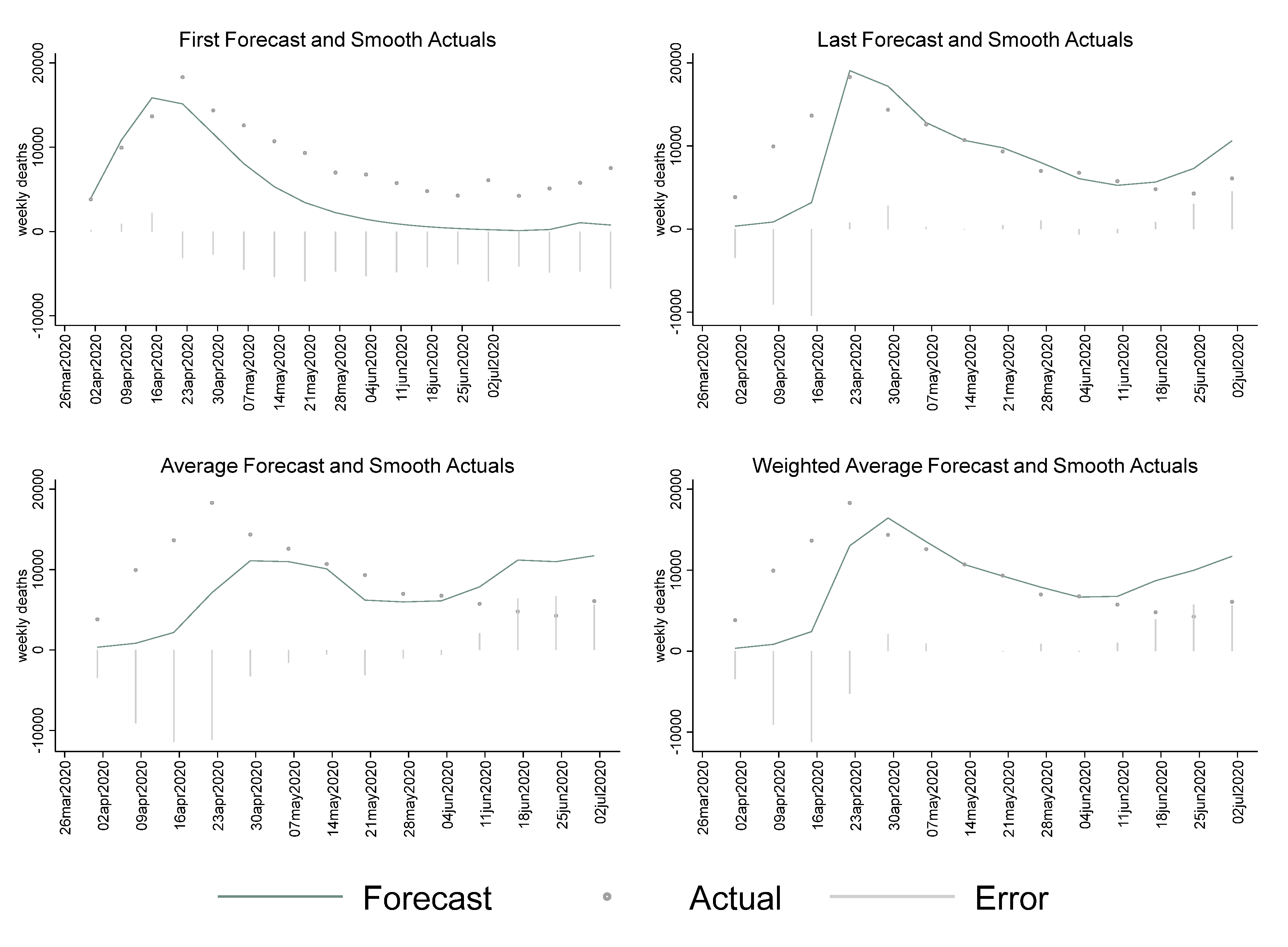
To evaluate the MIPH and IHME data, they were combined into one forecast following four different approaches. Two composite forecasts were made: (1) When there were two or more forecasts, the first forecast made was treated as the forecast; this procedure roughly reflected expectations, as seen by those external to forecast making, which might include policymakers; (2) When there were two or more forecasts, the last forecast was treated as the forecast; this reflected the general perception of forecasters and might reflect external expectations after longer intervals. In addition, two averages were calculated; (3) an unweighted average and (4) a weighted average with a weight (1 > w > 0) favoring the most recent forecast and exponentially declining for earlier forecasts, absorbing the remaining weight in the oldest forecast. The weight factor was set at w = 0.5. As ensemble forecasts have been used extensively for COVID-19 [28,29], an additional set of forecasts were computed by averaging each of the four combined IHME forecasts with its match from the 70 percent contact forecast from Columbia University. Forecast averaging, or other forms of combining, is a well-established practice [30,31].

The data from Los Alamos National Laboratory and the University of Texas at Austin was collected through October 2020, which was the beginning of the second wave of COVID-19 infections and deaths in the U.S. Using this data, we examined whether the forecasts improved over time as more data became available and forecasters gained a better understanding of models and assumptions. The forecasts were evaluated with the following error measures where $F_t$ = Forecast, $A_t$ = Actual values for a particular date, and $n$ = number of forecast periods. Following [4], we calculated a series of error measures:

$$\mathit{Mean}\mathit{Error} (\mathit{ME})=\frac{1}{n}{{\displaystyle \sum }}_{t=1}^n(F_t-A_t)$$

$$\mathit{Mean}\mathit{Percent}\mathit{Error} (\mathit{MPE})=\frac{1}{n}{{\displaystyle \sum }}_{t=1}^n\frac{(F_t-A_t)\ast 100}{A_t}$$

$$\mathit{Mean}\mathit{Absolute}\mathit{Percent}\mathit{Error} (\mathit{MAPE})=\frac{1}{n}{{\displaystyle \sum }}_{t=1}^n\frac{|(F_t-A_t)|\ast 100}{\left|A_t\right|}$$

$$\mathit{Symmetrical}\mathit{Mean}\mathit{Absolute}\mathit{Percent}\mathit{Error} (\mathit{SMAPE})=\frac{1}{n}{{\displaystyle \sum }}_{t=1}^n\frac{|(F_t-A_t)|}{(F_t+A_t)/2}$$

$$\mathit{Root}\mathit{Mean}\mathit{Squared}\mathit{Error} (\mathit{RMSE})=\sqrt[2]{\frac{{{\displaystyle \sum }}_{t=1}^n{(F_t-A_t)}^2}{n}}$$

As even the most cursory review of the graphic data shows, there was a weekly seasonal pattern in the daily death count. This pattern appeared to reflect the relative access to health care (and, thus, observation) available during the working week compared to the weekend. We compared the forecasts against the weekly moving average of mortality and calculated the errors, as well as depicted them graphically on a daily scale. Alternatively, we also examined the total deaths summed for each week. The weekly analysis was informative but had very few observations, since our core analysis of IHME and MIPH data focused on only three early months of the pandemic, reported in Appendix A.

Another important consideration was how far into the future the agencies could reliably forecast COVID-19 mortality. To examine this issue, we reported average and percent error for IHME and MIPH, using subsamples of weekly horizons. The MIPH data consistently made 41-day forecasts, so we organized the results into six weeks. The IHME model, on the other hand, had a longer forecast horizon of up to 12–16 weeks, but, in the early months, errors were significantly large in the later weeks, so we did not report results beyond the 8-week horizon. To examine whether forecast performance improved over time, we used the data from Los Alamos National Laboratory and the University of Texas at Austin. We divided the data into bi-monthly periods for the first six months of the pandemic, i.e., until the end of the first wave, and calculated disaggregated mean error and mean absolute percent error. The next section summarizes the key results in the graphs and tables.

4. Results and Discussion

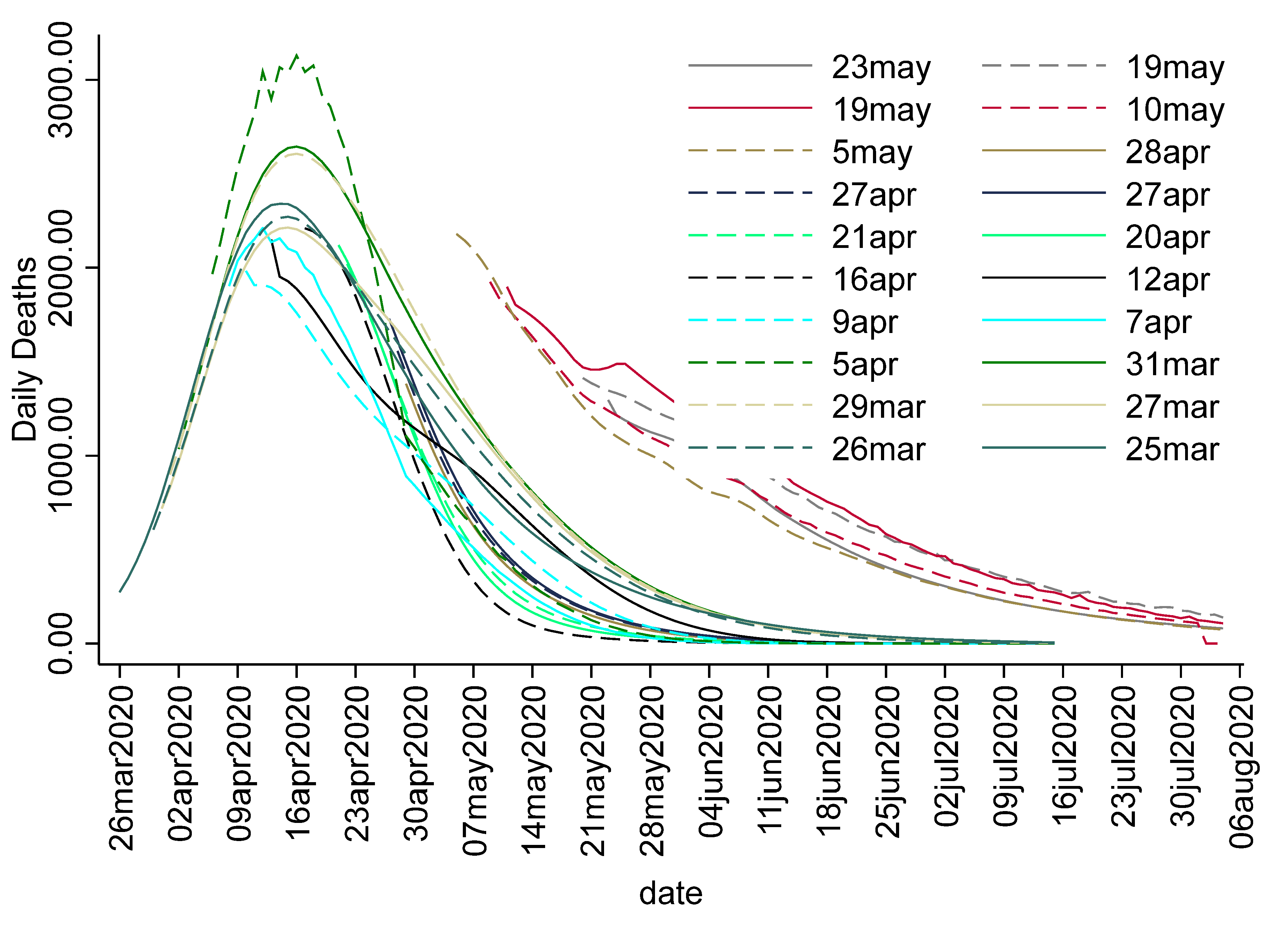
A comparative assessment of IHME and MIPH forecasts showed significant variation, depending on the forecast aggregation technique and underlying assumptions about social distancing. Figure 1 shows an overlay of the 22 IHME forecasts from the first forecast during early days of the pandemic through the end of the series (beyond the end of the evaluation period during the initial months of the pandemic). Except for the last few, these forecasts were similar with the right-hand tail expanding up the X axis as later forecasts were made. This expansion was substantially higher for the last five forecasts.

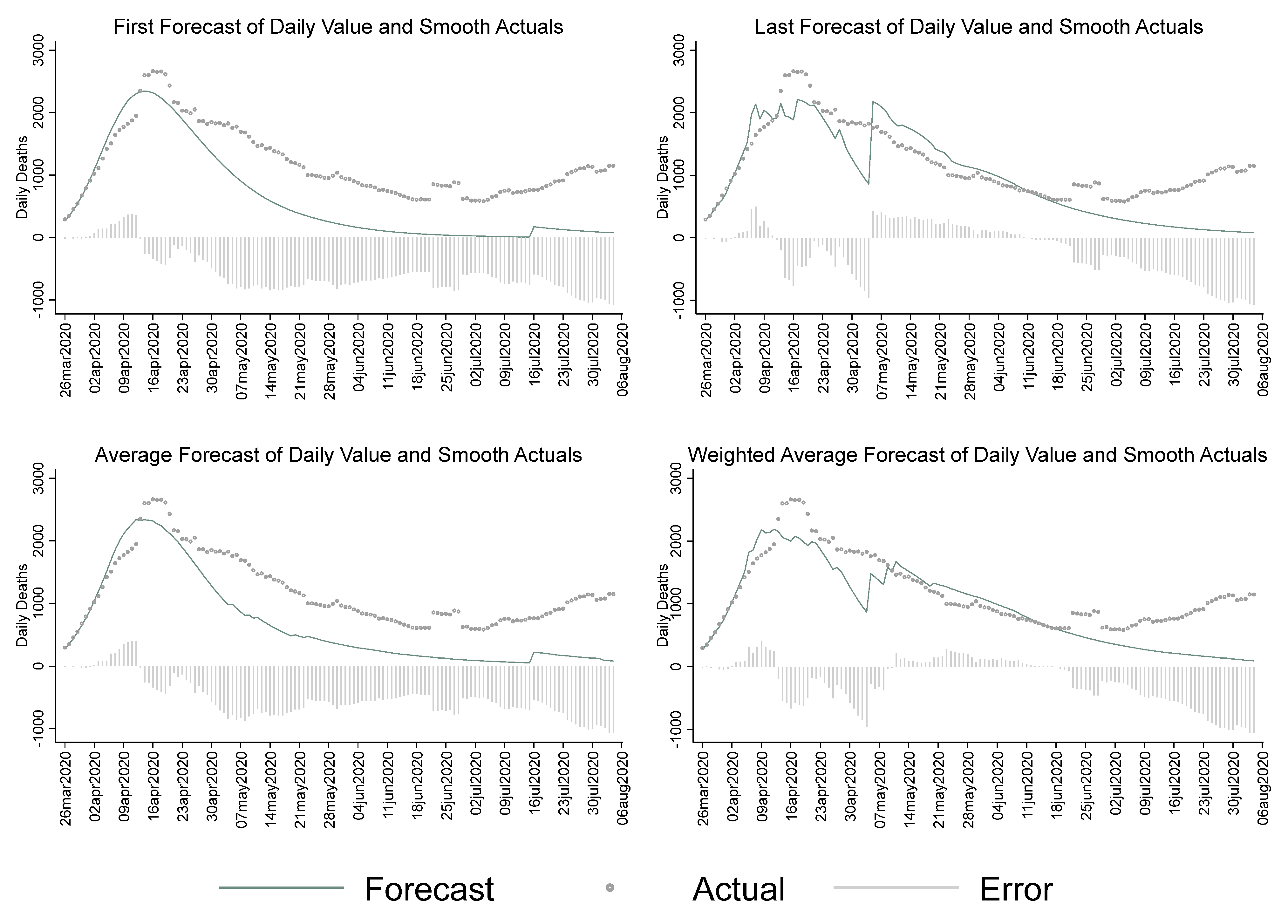
However, the predictions by the IHME for the right-hand tail were significantly underestimated, as shown in Figure 2, which compares the four combined forecasts with the actual data, as reported by CSSE through August 2020. For the period beginning around May 7th, the first forecast, and much of the influence of many of the other forecasts. as shown in the average, produced a much lower forecast for later periods than was found with the last forecast and the weighted average. IHME was the key forecast that was used in the White House Press Briefings on the pandemic situation, and appeared to have shown an optimistic picture (underestimated the number of deaths) in the spring and summer of 2020. This had significant implications for how the non-pharmaceutical recommendations were implemented at the national and local levels. For instance, the CDC guidance on non-medical face coverings for the general public was not issued until 3 April 2020. More accurate early forecasts from organizations that were informing government policy might have led to prompt action in such matters. Comparatively, while MIPH data, shown later, exhibited some large errors, including underestimation in the early period, it more accurately reflected the early summer period, which might have led to more aggressive action early on.

Table 2. Aggregated Error Measures for IHME and MIPH Forecasts.

Model/Aggregated (Multiple Forecasts)	ME	MPE	MAPE	SMAPE	RMSE
IHME
Composite with first forecast of daily value	−558.6	−58.90%	61.34%	104.79%	655
Composite with last forecast of daily value	−215.5	−22.56%	34.15%	49.37%	470
Average of forecasts by day	−516.6	−53.45%	55.63%	88.52%	449
Average with exponentially declining weights	−242.1	−22.91%	31.28%	44.78%	0
MIPH no intervention
Composite with first forecast of daily value	7824.7	707.45%	755.79%	135.76%	17,196
Composite with last forecast of daily value	167.0	30.90%	67.79%	55.20%	920
Average of forecasts by day	3060.9	270.23%	306.43%	121.69%	4864
Average with exponentially declining weights	566.0	75.89%	110.23%	76.11%	1194
MIPH 80
Composite with first forecast of daily value	1938.1	168.74%	224.88%	104.93%	4861
Composite with last forecast of daily value	143.2	29.75%	68.85%	57.69%	952
Average of forecasts by day	491.9	76.48%	118.65%	83.56%	1342
Average with exponentially declining weights	285.4	53.82%	92.18%	68.22%	1121
MIPH 70
Composite with first forecast of daily value	1462.7	109.94%	183.10%	109.81%	4676
Composite with last forecast of daily value	−109.9	−4.38%	36.03%	46.47%	640
Average of forecasts by day	−51.6	−11.49%	59.24%	64.54%	852
Average with exponentially declining weights	−93.5	−3.22%	42.84%	51.84%	688
MIPH 60
Composite with first forecast of daily value	119.7	28.36%	114.72%	110.09%	1651
Composite with last forecast of daily value	−59.3	−4.09%	45.20%	51.43%	720
Average of forecasts by day	−197.5	−8.17%	66.84%	68.54%	902
Average with exponentially declining weights	−44.1	−13.14%	54.28%	57.08%	788
Averaged IHME and MIPH 70
Composite with first forecast of daily value	798.7	45.00%	111.83%	75.44%	3414
Composite with last forecast of daily value	−109.1	−6.53%	23.75%	29.38%	468
Average of forecasts by day	−184.7	−7.44%	33.28%	38.93%	584
Average with exponentially declining weights	−122.6	−3.21%	27.42%	32.61%	500

reports the error measures for the four combined IHME forecasts. These show the “last” forecast made, and the weighted average favoring the last forecast, substantially outperformed the “first” forecast made or the average of all forecasts. However, the estimated mean errors (MEs) and mean percent errors (MPEs) of all approaches showed that IHME significantly underestimated mortality attributable to the pandemic. Mean Absolute Percent Error, however, remained relatively stable across estimation approaches. MAPE is an asymmetric metric that has no bounds for forecasts that are higher than actuals. We calculated the SMAPE that addressed this issue. For IHME, the difference between MAPE and SMAPE was higher for the first forecast than for the last forecast.

The mean errors for MIPH data vary across the social distancing assumptions. The largest errors obviously arose under the “no intervention” assumption, which was indeed not true, due to policy changes of closures and shutdowns enacted in March 2020. MIPH60, the most conservative contact assumption, came closest to actual levels of changes in mobility in the United States, as per Google Community Mobility Reports, which could be used as a proxy for infectious contacts. Therefore, we primarily focused on MIPH 60 for comparisons with IHME, but the error measures of all the contact thresholds are reported in Table 2. 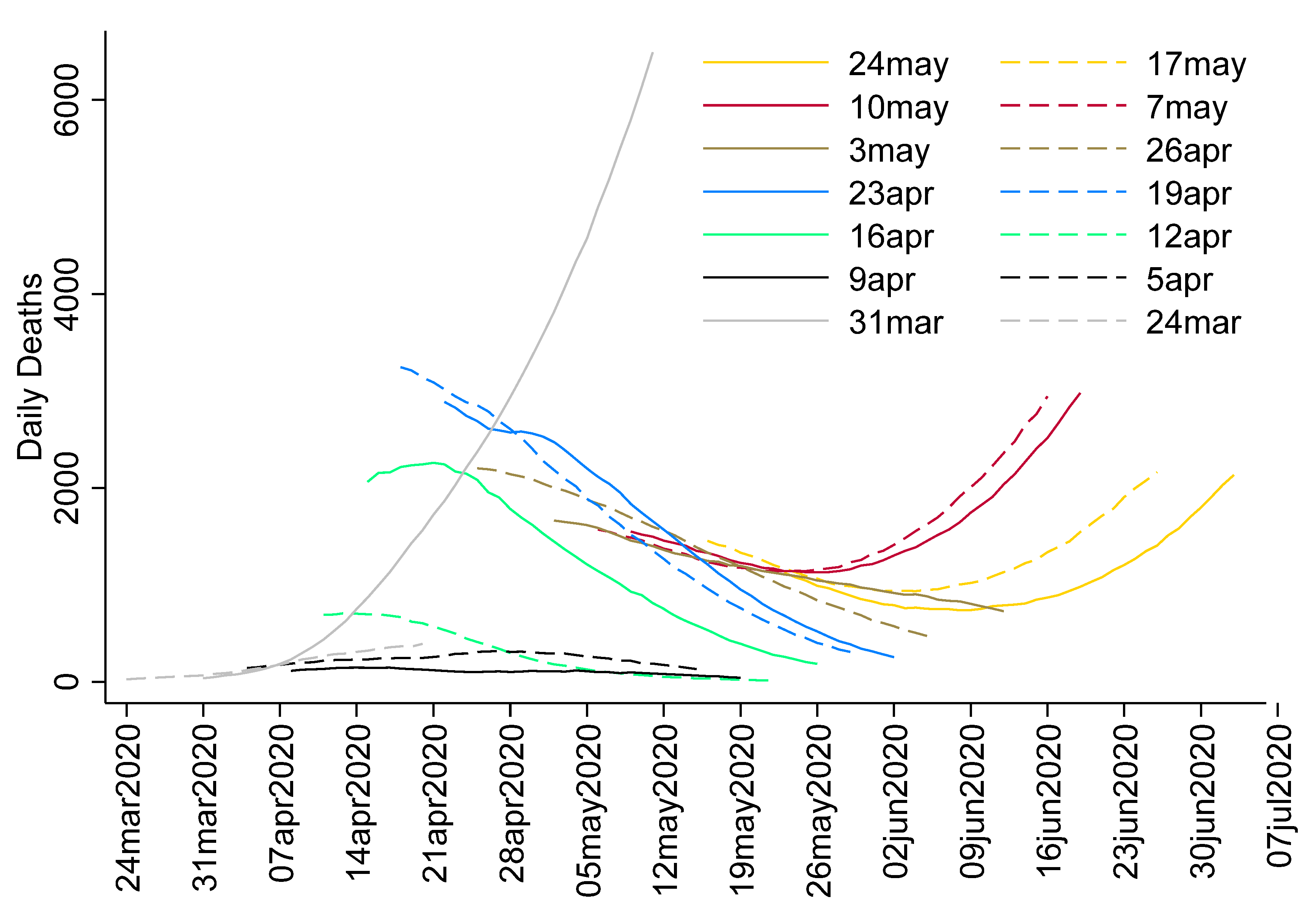Figure 3 shows the forecasts as made over various dates by MIPH, which showed remarkably high forecasts on the beginning date of 31 March 2020, sharply dwarfing all other forecasts. 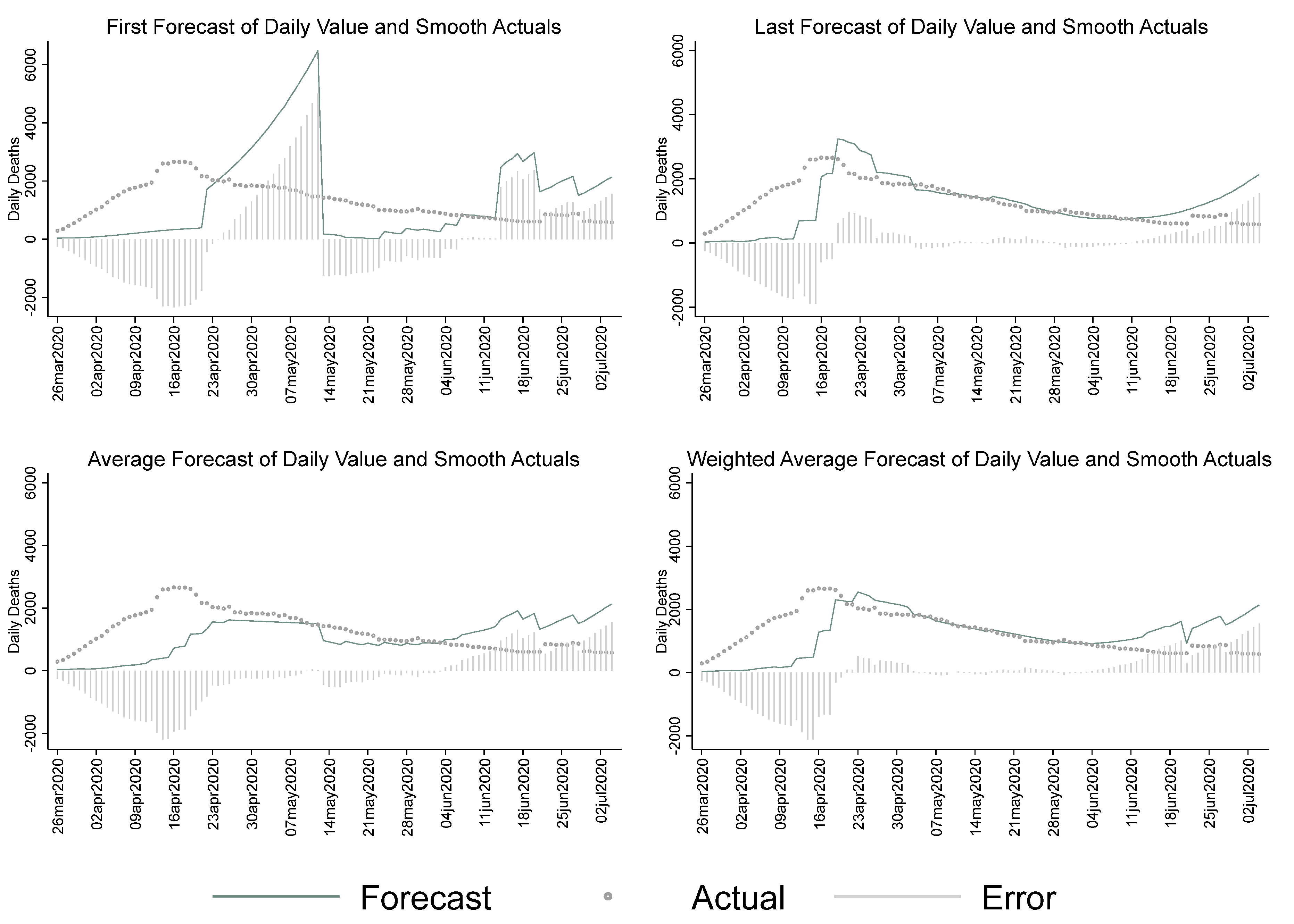Figure 4 shows the combined MIPH forecast against the weekly moving average of actual deaths. One thing that can be observed is that the forecasts substantially lagged behind the actual data in the early period. Similarly, the “first” forecast composite, substantially overran the actual data. MIPH, however, did not tend to flatten the curve at the tail-end of the summer, even under the 60 percent contact assumption, which suggested that the model was fairly more reliable in predicting the trajectory of the pandemic, as compared to the IHME model.

Table 2 reports detailed error measures across the physical contact thresholds for MIPH data as well. MIPH 60 was the only physical contact threshold that had a consistently negative ME/MPE across the estimation approaches. The average of forecasts by day was lowest for MIPH 60 and error measures were highest for the “no intervention” category. MIPH 60 had lower mean errors than IHME and did a better job of predicting mortality, on average, but the MAPE values were higher for MIPH 60 than for the IHME forecasts.

In summary, for the period examined, the IHME forecasts outperformed the MIPH forecasts, regardless of which set of assumptions MIPH used. This also held true for the average between the two forecasting groups. However, visual inspection of the MIPH forecasts suggested certain anomalous forecasts that, if eliminated, might result in a beneficial effect of combined forecasts. In a secondary finding, the method of combining forecasts of the same series using the same assumptions in the form of always using the most recently made forecast generally outperformed other methods of working with frequently updated forecasts; however, it was essentially tied with using a weighted forecast with exponentially declining weights. Due to current research timelines, only one arbitrary initial weight was considered.

We also created the weekly aggregates of the MIPH60 and IHME forecasts to assess the weekly forecast performance. Due to the short time frame of the early COVID-19 forecasts, we had a limited number of weeks. These results are reported in the Appendix A,

Table A1. Weekly Aggregated Error Measures for IHME and MIPH Forecasts.

Model/Aggregated (Multiple Forecasts)	ME	MPE	MAPE	SMAPE	RMSE
IHME
Composite with first forecast of daily value	−3764.1	−57.03%	60.35%	101.87%	4456
Composite with last forecast of daily value	−1250.2	−18.97%	30.28%	42.24%	2832
Average of forecasts by day	−3462.1	−51.44%	54.32%	85.12%	4117
Avg with exponentially declining weights *	−1451.7	−19.46%	27.54%	38.13%	2807
MIPH no intervention
Composite with first forecast of daily value	55,776.4	122.44%	232.16%	232.16%	113,389
Composite with last forecast of daily value	531.8	141.94%	158.47%	136.33%	4696
Average of forecasts by day	21,409.2	112.41%	204.00%	188.05%	33,653
Avg with exponentially declining weights	3409.8	137.54%	169.62%	155.36%	7194
MIPH 80
Composite with first forecast of daily value	13,308.6	154.41%	222.21%	222.21%	31,804
Composite with last forecast of daily value	359.9	154.55%	177.79%	162.53%	4979
Average of forecasts by day	2875.3	144.83%	217.27%	202.89%	8404
Avg with exponentially declining weights	1385.9	149.86%	197.89%	183.30%	6610
MIPH 70
Composite with first forecast of daily value	10,367.9	209.27%	273.41%	273.41%	30,546
Composite with last forecast of daily value	−977.6	−160.59%	180.63%	169.27%	3853
Average of forecasts by day	−556.5	−180.57%	205.39%	198.59%	5698
Avg with exponentially declining weights	−859.4	−165.65%	189.04%	181.66%	4384
MIPH 60
Composite with first forecast of daily value	535.1	347.61%	393.96%	393.96%	10,611
Composite with last forecast of daily value	−756.5	−166.60%	206.09%	188.53%	4188
Average of forecasts by day	−1753.1	−240.41%	266.08%	226.01%	5961
Avg with exponentially declining weights	−646.8	−179.09%	213.85%	200.62%	4895
Averaged IHME and MIPH 70
Composite with first forecast of daily value	12,588.2	130.95%	130.95%	95.06%	19,630
Composite with last forecast of daily value	8424.6	93.61%	93.61%	95.50%	9321
Average of forecasts by day	7277.4	82.64%	82.64%	0.00%	7981
Avg with exponentially declining weights	8316.0	96.58%	96.58%	96.54%	8909

. The facet plots in Figure A1 show weekly errors for the first forecast, last forecast, average, and weighted average. Generally speaking, the weekly patterns were consistent with the daily patterns for IHME and MIPH60. The first forecasts of the IHME model consistently underestimated on a weekly scale as well, but had much smaller absolute errors than MIPH60, as shown in Table A1.

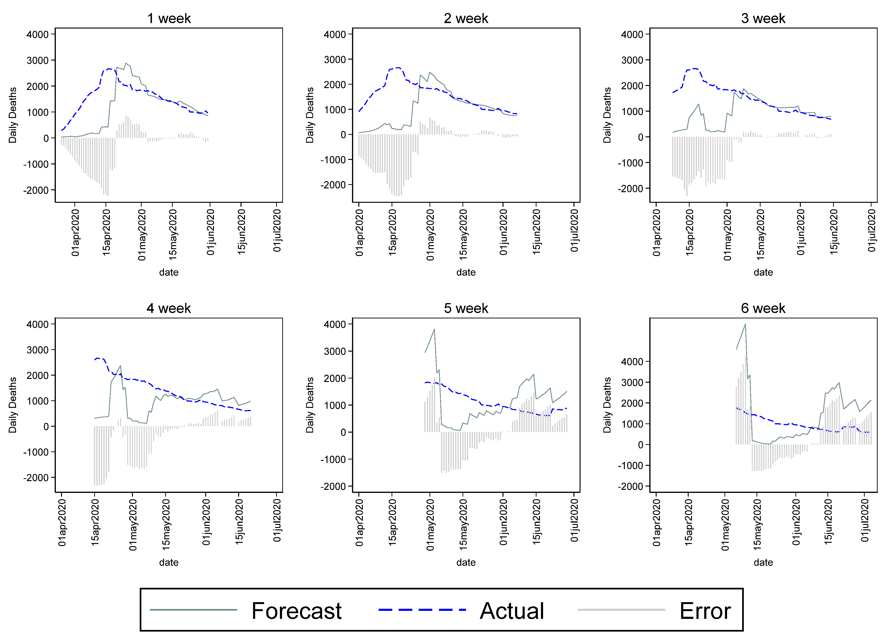
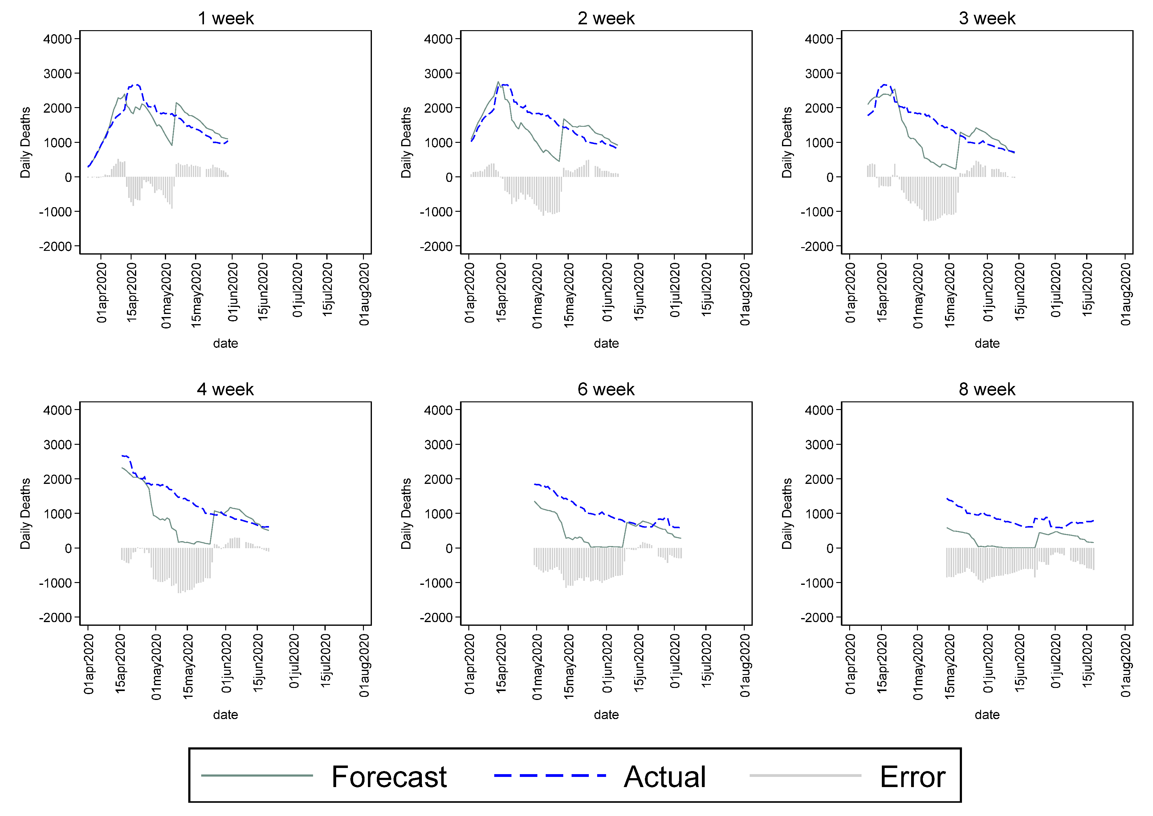
Another issue of interest was the accuracy of the forecasts over different forecasting horizons. Figure 5 and Figure 6 plot the forecasts and actuals for MIPH60 and IHME that were stratified over weekly forecasting horizons. Since the MIPH forecasts had a consistent 41-day forecasting window, we stratified the data over six weeks, as shown below. In the early days of the pandemic, the forecasters struggled to make even short-term forecasts and errors were significantly large. 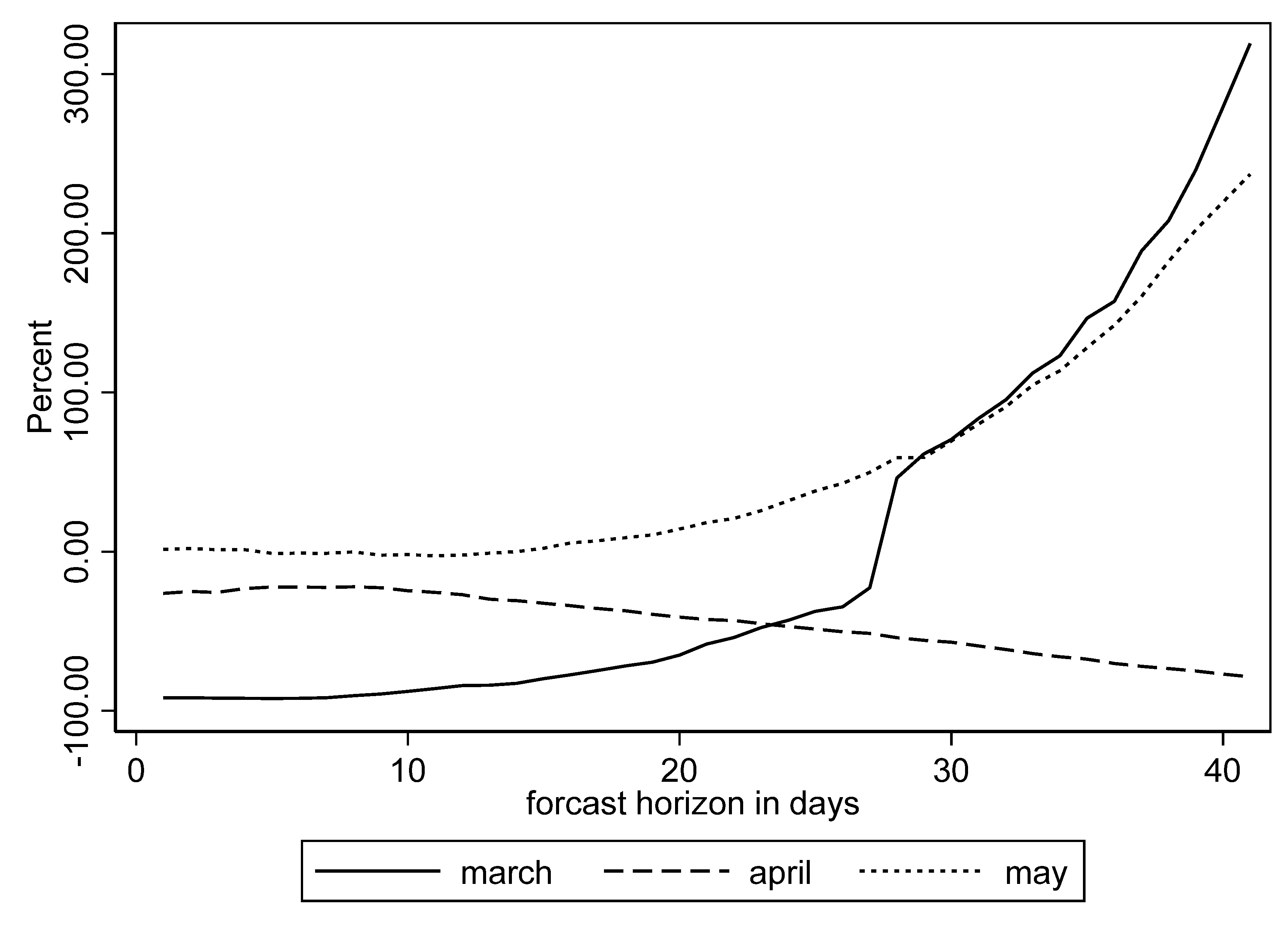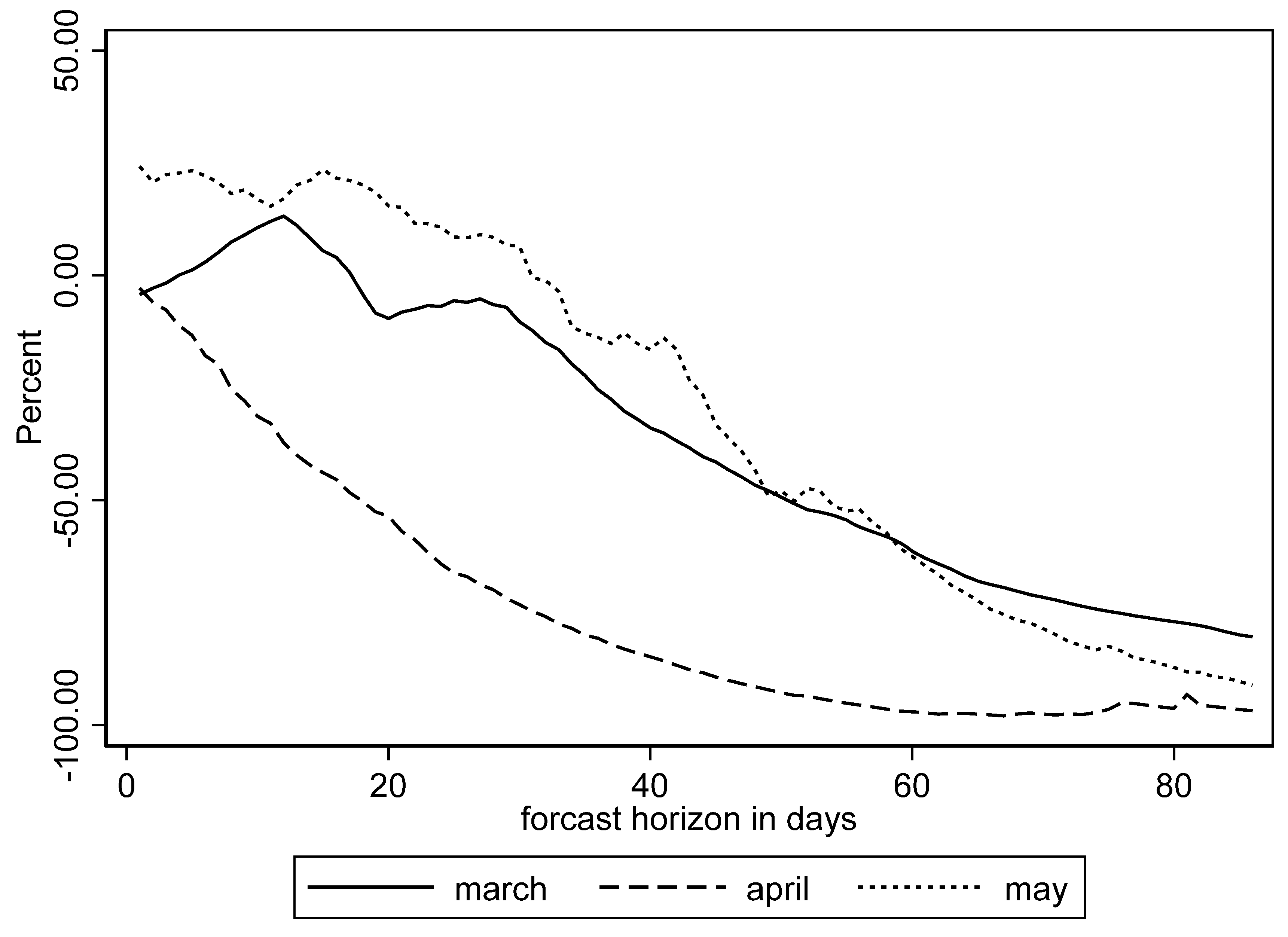However, as the pandemic progressed, and some information about the dynamics of virus transmission, such as value of R₀, became available, the forecasts had improved by the end of April. After that, the 1-week, 2-week, and 3-week forecasts were not significantly different for MIPH60, but the errors were relatively larger beyond that. The errors for IHME also tended to get considerably larger around the 3 to 4-week mark. Due the variation in the mortality data, percent errors did a better job of depicting the changes in forecast horizon trends. We plotted percent errors in for the two forecasters and stratified the data monthly for the first three months of the pandemic in Figure A3 and Figure A4 in the Appendix A. Figure A3 shows an apparent increase in MIPH60 errors beyond the 3-week forecasting horizon. The patterns for IHME varied much more significantly across the months of forecasts, but the errors tended to increase significantly for IHME as well, beyond the 3 to 4-week mark. In summary, the results of stratifying over forecasting horizons suggested that COVID-19 mortality forecasts beyond three weeks were subject to significant errors, but the IHME and MIPH models improved as the first wave progressed.

The MIPH and IHME forecasts used in this study started providing forecasts early on in the pandemic and might have influenced public behavior and government policy. In the subsequent months, other forecasters, such as the University of Texas, Austin and Los Alamos National Laboratory, also joined the fray, so we did not compare them directly to IHME and MIPH. The forecasts from mid-April by these organizations had the benefits of knowing the government policy, more data, and the trajectory of previous estimates by IHME and MIPH and other early forecasters. Therefore, these agencies had, on average, significantly lower mean error and mean absolute percent error than the early forecasters. 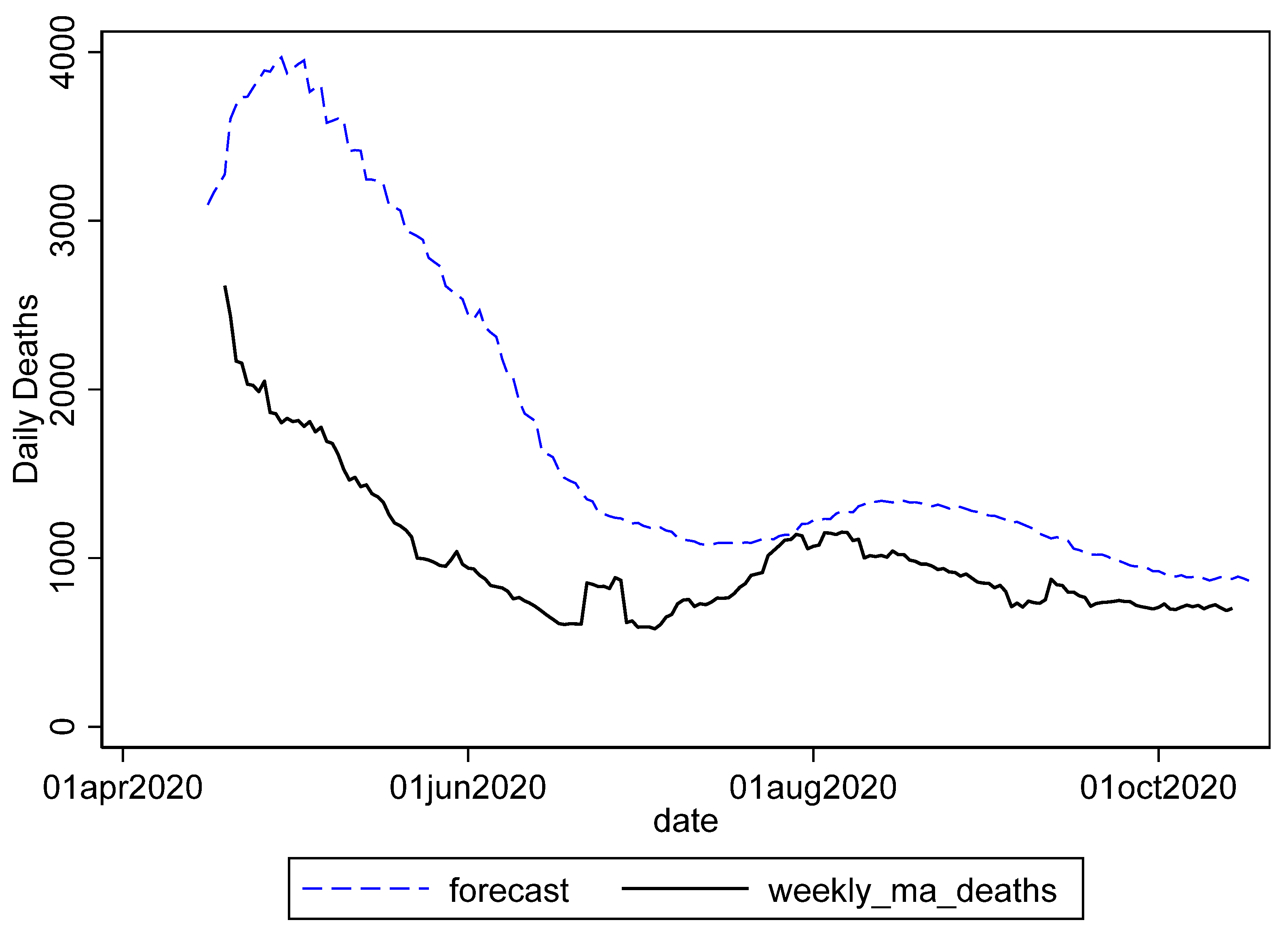Figure 7 plots the Los Alamos National Laboratory forecasts with actual mortality between mid-April to early October. The curve-fitting model used by LANL had larger errors in the initial months, and, as the pandemic progressed, the errors became significantly lower. The LANL model also tended to over-forecast mortality throughout the first wave of the pandemic, but the errors reduced significantly after June 2020. The upper bound of the UT-Austin forecast had significant errors and outliers, so, therefore, we reported the upper and lower bounds separately (Figure 8). While the errors were significant in the early months, the UT-Austin forecast performed well in June and July. Their forecast was also relatively efficient in predicting the spike in the early weeks of the second wave of the pandemic.

The key error measures, namely, MPE and MAPE, for the average of forecasts by LANL and UT-Austin are reported in

Table 3. Average Errors LANL and UT-Austin Forecasts, Smooth Aggregates and Bi-Monthly.

	Mean Percent Error (MPE)		Mean Absolute Percent Error (MAPE)
	LANL	UT-Austin	LANL	UT-Austin
Average of forecasts by day	14.65	11.23	28.05	31.07
		Bi-Monthly Errors
April–May 2020	39.32	11.90	59.60	38.71
June–July 2020	14.21	3.96	25.79	18.24
August–October 2020 *	7.56	32.20	20.30	43.02

* Until the first week of October 2020.

. The UT Austin model, which was a SEIR model that accounted for actual social distancing trends, had a lower mean percent error compared to the LANL model, which was a time-series model. These models differed from IHME and MIPH in that they significantly overestimated mortality. While the UT-Austin model had lower MPE, the LANL model had lower MAPE, suggesting a higher forecast accuracy.

These models also improved over time, as more data about virus transmission became available. Table 3 also reports ME and MAPE for bi-monthly forecasts from mid-April to the beginning of October. The mean percent error significantly reduced as the pandemic progressed and forecasters had an opportunity to validate their models and assumptions. Mean percent error in LANL estimates reduced from 39.32 percent during the April–May period to 14.21 during the June–July period, and subsequently to 7.56 in the August to early October period. We see a similar decline in UT-Austin estimates in the June–July period, but the errors increased in the subsequent period. UT Austin suspended publishing forecasts and undertook a change in their methodology during this period that could potentially explain this variation. The estimates of absolute error were also consistent and suggested that forecast accuracy improved as the pandemic progressed, but the second wave again tested the reliability of these models, which could be explored in future research.

5. Conclusions

This study examines the forecasts of four major agencies that provided COVID-19 forecasts in the initial months of the pandemic in the United States. First, we compared the forecasts of two agencies, IHME and Columbia University, that actively produced forecasts in the early days of the pandemic and were instrumental in shaping public behavior and government policy. We found that the IHME forecasts sharply underestimated mortality. However, we found that the forecasts made by IHME better reflected the actual progression of COVID-19 deaths in the United States, but this could be because it was picking up underlying social distancing trends. MIPH forecasts, on the other hand, were widely discussed and influenced the behavior of the public at large. Thus, the very large expansion rates shown in the early MIPH might have had a causal relationship with the subsequent public self-sequestering and quarantine, which ultimately led to their deviating from actual data. It is, nevertheless, remarkable that for the earliest MIPH forecasts, even the forecasts of the most aggressive intervention, far overshot the actual instances of death. Two possible considerations are: (1) there is a widespread belief that failure to test, particularly of people who died before receiving medical attention, may have resulted in systematic undercounting of the actual death rate [32,33], and (2) actual response, such as self-sequestering, may have exceeded the most aggressive level forecast in the localities that were early hotspots of the pandemic. These concerns muddied the ability to refer to accuracy, as opposed to the efficacy, of pandemic forecasting in motivating behavioral change. We also examined the forecasts of Los Alamos National Laboratory and the University of Texas at Austin and found that they had significantly lower mean errors compared to MIPH and IHME, the plausible explanation was that they were late entrants and had better data available when they started forecasting. The forecasts from the University of Texas at Austin had a lower mean percent error than the forecasts of the Los Alamos National Laboratory, while the LANL model had lower absolute errors. Mean percent error in the early months of the pandemic was higher and reduced as more information became available and models and assumptions were possibly revised. We also found that forecasts of the pandemic beyond 3–4 weeks produced much larger errors and tended to be unreliable. However, more research and an inquiry into the second-wave forecasts could possibly shed light on this finding.

Lastly, the forecasts from the Columbia University and University of Texas, Austin were based on SEIR models, and the models used by the IHME and LANL relied more on curve-fitting approaches. The results suggested that errors in both SEIR models (using MIPH60 as the reference) were lower than the IHME and LANL. However, IHME and LANL models had lower mean absolute percentage error. This could suggest that the SEIR models were effective in predicting the trajectory and direction of the pandemic, while the curve fitting approaches might have had higher short-term forecast accuracy. Comparative analysis of more forecasts by different agencies could provide more insights, having implications for the practice of ensemble forecasting, which organizations like the Center for Disease Control and Prevention are actively using to aggregate forecasts.

There are several limitations of this analysis that we would like to highlight. First, the data availability limited the scope of forecast comparison, since the timelines and approaches varied significantly. Second, the social distancing assumptions and actuals varied substantially across models, rendering some forecasts, such as several thresholds of MIPH, less useful for comparisons. Third, we did not adjust for seasonality in COVID-19 transmission patterns since we were exclusively focusing on six months during the first wave of the pandemic, but any longer-term forecast evaluation should account for seasonality in COVID-19 infections and mortality. Fourth, we mostly used the central tendency of forecasts, but the forecasters, in most instances, provided a range under different assumptions and comparisons of point estimates had inherent disadvantages. Fifth, the evaluation of these forecasts rested on the assumption that the reported mortality by the CSSE was accurate, which we now know was often not the actual number of deaths, given the large number of studies documenting excess mortality due to COVID-19. Lastly, as the pandemic evolved and health systems became more prepared, a reduction in mortality was evident, and it would have been challenging for any forecast to significantly account for variation in policy responses.