Integrating Ecological Forecasting into Undergraduate Ecology Curricula with an R Shiny Application-Based Teaching Module

Abstract

Ecological forecasting is an emerging approach to estimate the future state of an ecological system with uncertainty, allowing society to better manage ecosystem services. Ecological forecasting is a core mission of the U.S. National Ecological Observatory Network (NEON) and several federal agencies, yet, to date, forecasting training has focused on graduate students, representing a gap in undergraduate ecology curricula. In response, we developed a teaching module for the Macrosystems EDDIE (Environmental Data-Driven Inquiry and Exploration; MacrosystemsEDDIE.org) educational program to introduce ecological forecasting to undergraduate students through an interactive online tool built with R Shiny. To date, we have assessed this module, “Introduction to Ecological Forecasting,” at ten universities and two conference workshops with both undergraduate and graduate students (N = 136 total) and found that the module significantly increased undergraduate students’ ability to correctly define ecological forecasting terms and identify steps in the ecological forecasting cycle. Undergraduate and graduate students who completed the module showed increased familiarity with ecological forecasts and forecast uncertainty. These results suggest that integrating ecological forecasting into undergraduate ecology curricula will enhance students’ abilities to engage and understand complex ecological concepts.

1. Introduction

Rapid changes in many ecological populations, communities, and ecosystems due to land use and climate change has motivated the emerging discipline of near-term, iterative ecological forecasting [1,2,3,4,5]. We define near-term ecological forecasting as the prediction of future (day to decade) environmental conditions with quantified uncertainty [6]. Ecological forecasting has much potential for advancing ecology as a discipline because it can both improve decision-making related to natural resource management and expand knowledge of ecological systems [2,7,8,9]. As an example, if managers had advance warning of an algal bloom in a drinking water reservoir, they could preemptively adjust the depth of outtake of water or treat the water to avoid or mitigate deteriorating water quality [1,10].

An important part of near-term ecological forecasting is the iterative forecasting cycle, in which forecasts are updated as new observations become available. The iterative, near-term ecological forecasting (INTEF) cycle consists of multiple steps (Figure 1): (1) creating a hypothesis of how an ecological variable changes in the future; (2) developing a mathematical model to predict the future dynamics of the variable using collected field observations; (3) quantifying uncertainty in predictions; (4) generating a forecast with quantified uncertainty; (5) communicating the forecast to stakeholders; (6) assessing the forecast when new observational data are available; and (7) updating the forecast with new data (e.g., changing model parameters, initial conditions) to improve the model for the next forecast. This cycle is then repeated each time a new forecast is made [11]. Collection of observational data is critical for steps 1, 2, 6, and 7 and, therefore, is an integral part of ecological forecasting. This iterative cycle enables the development of better ecological models and improved ecological understanding [12]. It also allows for proactive, rather than reactive, management for preparing for future environmental conditions, decision-making, and implementing policies [13].

Ecological forecasting offers a compelling and engaging tool for enriching undergraduate ecology education. First, integrating near real-time ecological data into the classroom for hands-on analyses and forecasting engages students in authentic research experiences, thereby increasing students’ conceptual understanding of ecology [14,15,16]. Second, the immediate application of forecasting for improving natural resource management can engage ecology students interested in actionable and applied science, especially via scenario and problem-based learning exercises, which can enhance both students’ interest in, and understanding of, ecology [17]. Third, ecological forecasting provides a platform for teaching students critical quantitative, modeling, and data science skills, which are needed for a range of careers in multiple sectors. The U.S. Bureau of Labor Statistics estimates that data science positions are expected to increase by 28% from 2016 to 2026 [18]. As a result, there is a strong incentive to develop ecology undergraduate curricula which cover this broad range of quantitative skills to prepare students for careers in this field. Fourth, forecasting has been identified as an “environmental imperative” by the U.S. government [19], providing a strong impetus for motivating future careers in this field, as exemplified by the expanding role of forecasting within the U.S. Geological Survey (USGS), National Oceanic and Atmospheric Administration (NOAA), and U.S. Centers for Disease Control (CDC).

While there are increasing opportunities for training graduate students in ecological forecasting and the INTEF cycle, ecological forecasting has yet to be integrated into undergraduate training, resulting in a potential gap in ecology curricula. For example, graduate student training in the skills needed for ecological forecasting has increased in recent years through development of the Ecological Forecasting Initiative (https://ecoforecast.org; accessed on 25 April 2022), student-led and targeted workshops (e.g., through the Global Lake Ecological Observatory Network; https://gleon.org, accessed on 25 April 2022), and classes specifically targeted at the graduate level (e.g., upper-level modeling and statistics courses).

However, similar ecological forecasting training opportunities do not exist at the undergraduate level. Teaching undergraduate ecology students the INTEF cycle is a powerful tool for reiterating fundamental scientific principles, as the forecasting cycle is the scientific method in practice and also introduces them to interdisciplinary applications of ecology and a broad array of research opportunities. The challenge of addressing all the embedded concepts within ecological forecasting (e.g., mathematics, statistics, data science, social science, ecological modeling, science communication) may explain why it has not yet been broadly adopted in undergraduate classrooms, in addition to the field’s recent development. Moreover, because the practice of ecological forecasting requires programming and modeling, skills rarely taught to undergraduates [20], the intimidation barrier to both teaching and learning forecasting may be high. New approaches are needed to integrate ecological forecasting into undergraduate classrooms to overcome these barriers of teaching INTEF at an appropriate introductory level. Specifically, INTEF teaching tools that do not require extensive programming or computational skills are critically needed to ensure that ecological forecasting training is accessible to introductory students, enabling them to master ecological forecasting concepts and introducing them to the complete INTEF cycle.

One pedagogical approach which may enable the teaching of ecological forecasting concepts and skills to undergraduate students is embedding interactive activities and lessons in a digital learning environment. This approach is widely used across many disciplines and educational levels, ranging from primary school to graduate level courses, particularly in statistics and other quantitative courses [21], as their interactive nature enhances student engagement and interest in these topics [22]. There are many different examples of interactive online tools that have been integrated into educational approaches, though we note that the effectiveness of these approaches vs. non-interactive online methods remains unresolved. For example, programming and coding activities in languages such as R may help students apply ecological concepts, use quantitative reasoning, and conduct modeling and simulation [23]. As an example, one short 3-hr lesson using the interactive R programming language improved senior undergraduate and graduate student comprehension of complex ecological concepts such as climate change and ecological simulation modeling [24]. However, the use of code-based applications such as R can often cause stumbling blocks for students as they struggle to debug code rather than focus on the ecological concepts of interest.

For introductory ecology students who likely have no or minimal programming skills, the recent advances in online applets and web applications (e.g., R Shiny applications) may provide a more useful interface for self-guided lessons for teaching forecasting than lessons which require extensive coding experience [25] and may build on the success of several other interactive online tools. These earlier tools include NetLogo, a multi-agent programmable modeling environment, which has been used to improve K–12 students’ knowledge of environmental science content and ability to interpret graphs [26]. NetLogo was also shown to be a useful tool in helping to correct misconceptions in inorganic chemistry at the university level [27]. Another example of an interactive online tool is the common online data analysis platform (CODAP), which has been integrated into the teaching of machine learning and other data science topics [28]. Interactive activities embedded in online applets facilitate students learning at their own pace, and self-discovery has been shown to improve students’ understanding and ability to retain information [29,30].

R Shiny applications provide an unprecedented level of customization for educators looking to embed interactive lessons into an online interface and are gaining in popularity in research and as a teaching tool [31]. R Shiny applications use a combination of HTML and JavaScript generated from R code [25] to support a high level of interactivity and are extremely flexible in their implementation. For example, R Shiny applications can be developed that enable users to load data from online repositories, visualize complex datasets, run a range of analyses, and build ecological models, among many other activities, all without needing to write code or work directly with a coding program. While there have been only limited studies on the use of R Shiny as a teaching tool to date, initial work indicates that embedding R Shiny applications into undergraduate curricula can increase students’ understanding and confidence in the subject matter by lowering the barrier to learning new concepts [32,33,34].

To assess the efficacy of an R Shiny application in teaching ecological forecasting and INTEF concepts to novice students, we developed a comprehensive 3-hour teaching module centered around activities embedded within an interactive online tool built with R Shiny. Importantly, students did not need any programming or complex modeling skills to complete the ~3-hour module. Within the module, the students explored data from an ecological site of their choice in the U.S. National Ecological Observatory Network (NEON), built a simple model that numerically simulated primary productivity for their site, and then used this model to generate short-term forecasts of productivity that were sequentially updated as additional data became available. Thus, students gained experience in ecological forecasting as they stepped through each component of the INTEF cycle. We assessed the module’s efficacy in teaching ecological forecasting concepts and meeting learning objectives (described below) using pre- and post-module surveys before and after module instruction at 10 universities and 2 conference workshops. We used the assessment data to answer the research question: how does embedding our teaching module into ecology curricula affect students’ ability to describe and understand ecological forecasting concepts?

2. Materials and Methods

2.1. Module Overview and Learning Objectives

The overarching goal of this module, titled “Introduction to Ecological Forecasting,” is to teach undergraduate students fundamental ecological forecasting concepts by interactively working through the INTEF cycle (Figure 1). The module’s learning objectives are: (1) Describe an ecological forecast and the iterative forecasting cycle; (2) Explore and visualize NEON data; (3) Construct a simple ecological model to generate forecasts of ecosystem primary productivity with uncertainty; (4) Adjust model parameters and inputs to study how they affect forecast performance relative to observations; and (5) Compare productivity forecasts among NEON sites in different ecoclimatic regions. Consequently, the module aimed to build students’ understanding of ecological data through exploratory visualizations, develop skills in how to create a hypothesis that could be instantiated as a mathematical model, as well as gain insight into ecological models, forecasting, and macrosystems ecology concepts.

The “Introduction to Ecological Forecasting” module is a stand-alone module targeted for introductory ecology students. All intermediate-level ecology concepts and principles are defined, therefore reducing the need for students to have any prior experience with ecosystem modeling, ecological forecasting, or NEON data. We used the INTEF cycle as described by the author of [11] as our primary conceptual model for teaching the steps of the INTEF cycle.

This module was part of the Macrosystems EDDIE (Environmental Data-Driven Inquiry and Exploration; MacrosystemsEDDIE.org) educational program. The goal of Macrosystems EDDIE is to teach the foundations of macrosystems ecology through modeling and forecasting. All of the Macrosystems EDDIE modules use the 5E Instructional Model [35], a pedagogical model in which students complete activities that enable engagement, exploration, explanation, elaboration, and evaluation. Each module consists of a short, self-contained suite of scaffolded activities that instructors can adapt to meet the needs of their lecture or laboratory class [16].

All Macrosystem EDDIE modules apply the Four-Dimensional Ecology Education (4DEE) Framework, which has been endorsed by the Ecological Society of America as a foundation for our modules [36,37]. Our module of focus here, “Introduction to Ecological Forecasting,” applies the 4DEE framework by integrating (1) core ecological concepts, such as ecosystem primary productivity (the response variable in the ecological model the students develop for forecasting) and trophic level interactions (nutrient–phytoplankton dynamics); (2) ecological practices, such as ecosystem modeling, data analysis, computational thinking, and ecological forecasting; (3) human–environment interactions, such as how resource managers can use ecological forecasts to aid their decision making; and (4) cross-cutting themes by viewing forecasting through a macrosystem ecology lens and comparing ecosystem productivity across temporal periods and sites spanning a large spatial extent.

2.2. Module Activities

The module was structured into four key parts. First, prior to class, instructors give students a short pre-module handout to read that introduces the module. The handout provides an overview on ecological forecasting and includes references for suggested readings and videos which they can view before the class. Second, at the beginning of the class, the instructor gives a brief (20-min) Microsoft PowerPoint presentation that introduces the key concepts and ideas for the lesson and an overview of the module’s activities. Key concepts that are defined in this presentation include ecological forecasting, the INTEF cycle, forecast uncertainty, and an introduction to a basic ecosystem primary productivity model. Third, the students work in pairs through the R Shiny application, which is accessible via any web browser on their or their partner’s computer. The students work together to complete three scaffolded activities (A, B, and C) embedded within the interactive online tool. These activities build from simple to more complex using the 5E learning cycle [38] (

Table 1. Overview of the conceptual structure of all EDDIE modules adapted from the authors of [37] and scaffolding of the Introduction to Ecological Forecasting module with a summary of the ABC activities within the module. See [35] for more information and module teaching materials. The module applies the 5E instructional model, with the 5Es (Engagement, Exploration, Explanation, Elaboration, Evaluation) italicized below.

Activity	EDDIE ABC Conceptual Framework	Introduction to Ecological Forecasting Module
A	Engage in initial data exploration and skill development using simple analyses	Engage in thinking about how forecasts are used and can advance ecological management. Explore NEON data from a site of the student’s choice and build a simple productivity model.
B	Explore and Explain through more detailed analyses and comparisons	Explore how the productivity model can best fit observations. Use the model to step through each stage of the forecast cycle. Explain the forecast and its uncertainty to a classmate.
C	Elaborate on developed ideas to other sites, datasets, and concepts. Evaluate knowledge in class discussion and homework	Elaborate on the forecasting framework by applying their model to generate a forecast for a different NEON site and compare results. Evaluate knowledge by answering discussion questions in the R Shiny app and together as a class.

). Within each activity, students complete multiple objectives, including data visualization, model analyses, forecast assessment, and forecast updating, with observations as they progress through the materials. Throughout the module, students complete 26 short-answer questions embedded in the interactive online tool that can be downloaded as a Microsoft Word file at module completion and submitted as an assignment at their instructor’s discretion. Fourth, instructors convene with the class following the completion of each A, B, and C activity to reflect and explain what they have done so far. This step also allows for the instructor to touch on key points which may have been missed by students as they worked through the objectives.

The module was specifically designed to achieve our five learning objectives (Section 2.1.). First, the goal of the lecture component was to present a comprehensive introduction to the INTEF cycle and provide an overview of the activities of the module. Learning objective 1 (Describe an ecological forecast and the iterative forecasting cycle) was introduced by the material in the lecture and reinforced throughout the objectives in Activity B. We included an inquiry activity in Activity A, in which students interacted with real “messy” ecological data from NEON and were able to visualize different relationships between the different ecological variables at their chosen NEON site, to achieve learning objective 2 (Explore and visualize NEON data). To achieve learning objective 3 (Construct a simple ecological model to generate forecasts of ecosystem primary productivity with uncertainty), we created a task in Activity A in which students used a simple ecological model to develop conceptual understanding of variable relationships in the model. Learning objective 4 (Adjust model parameters and inputs to study how they affect forecast performance relative to observations) was achieved by students comparing different forecasts with observations in Activity B to see how the forecast differs based on model parameterizations. Finally, to achieve learning objective 5 (Compare productivity forecasts among NEON sites in different ecoclimatic regions), students were tasked with re-running their model for a different NEON site in Activity C and answering class discussion questions.

A primary goal of the module is to have students recognize the benefits as well as challenges of using forecasts for a range of variables. Thus, before starting Activity A, the students complete some introductory questions in the R Shiny application on their use of forecasts in their daily lives, and they explore current existing ecological forecasts (e.g., USA National Phenological Network (NPN) Pheno Forecast, Grassland Production Forecast, Smart Reservoir Forecast). They select one of the pre-loaded existing forecast options and answer discussion questions regarding this forecast (all discussion questions are available in

Table A1. Short-answer questions which are embedded in the interactive online tool which the student must complete as they complete each of the different objectives within the activities.

Question Number	Question
1	How have you used forecasts (ecological, political, sports, any kind!) before in your day-to-day life?
2	How can ecological forecasts improve both natural resource management and ecological understanding?
3	How do you think forecasts of freshwater primary productivity will differ between warmer lakes and colder lakes?
4	Choose one of the ecological forecasts above and use the website to answer the questions below.
4a	Which ecological forecast did you select?
4b	What ecological variable(s) are being forecasted?
4c	How can this forecast help the public and/or managers?
4d	Describe the way(s) in which the forecast is visualized.
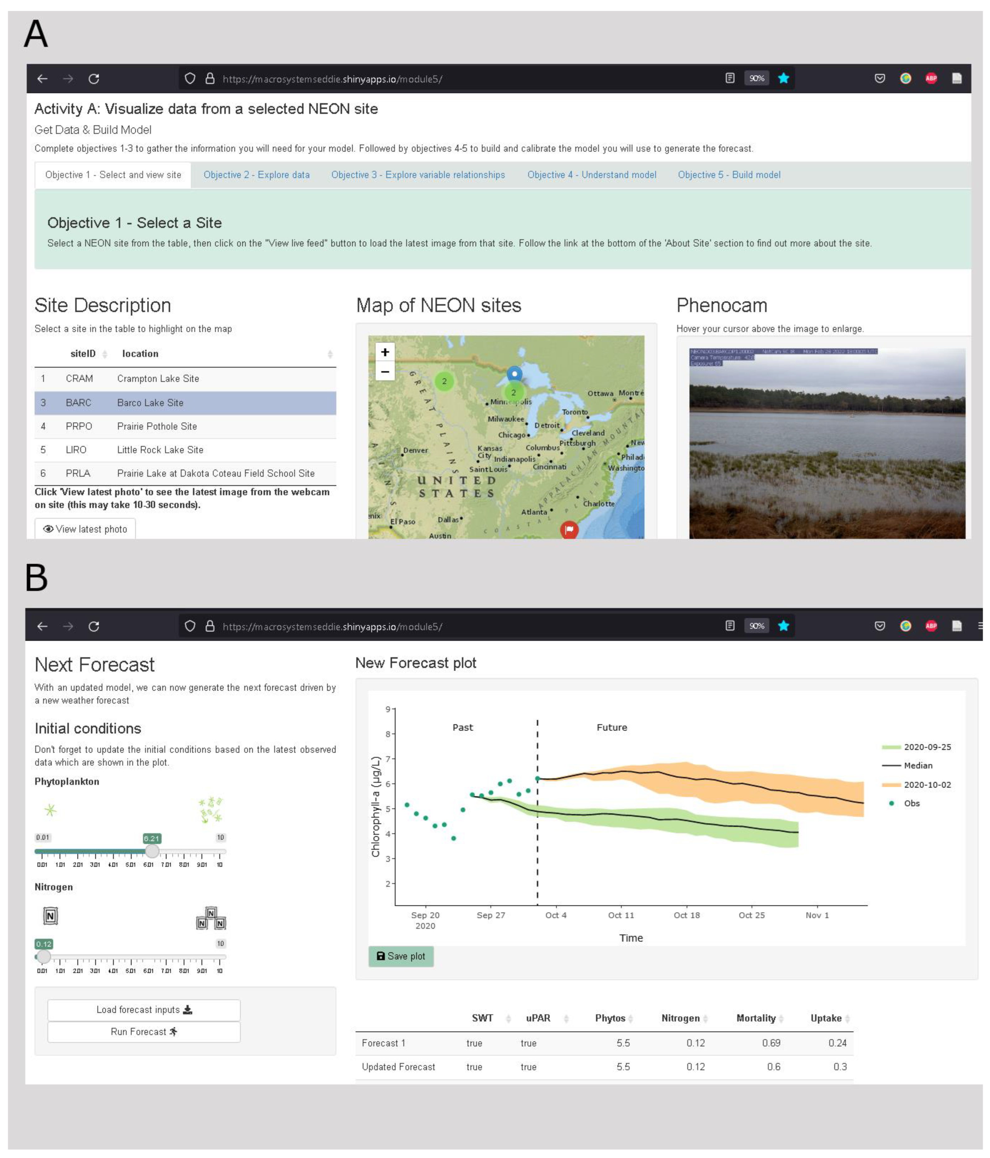
5	Fill out information about your selected NEON site:
5a	Name of selected site:
5b	Four letter site identifier:
5c	Latitude:
5d	Longitude:
5e	Lake area (km2):
5f	Elevation (m):
6	Fill out the table below with the description of site variables:
6a	Air temperature
6b	Surface water temperature
6c	Nitrogen
6d	Underwater PAR
6e	Chlorophyll-a
7	Describe the effect of each of the following variables on chlorophyll-a. Chlorophyll-a is used as a proxy measurement for phytoplankton concentration and primary productivity in aquatic environments.
7a	Air temperature
7b	Surface water temperature
7c	Nitrogen
7d	Underwater PAR
8	Were there any other relationships you found at your site? If so, please describe below.
9	What is the relationship between each of these driving variables and productivity? For example, if the driving variable increases, will it cause productivity to increase (positive), decrease (negative), or have no effect (stay the same).
9a	Surface water temperature
9b	Incoming light
9c	Available nutrients
10	Classify the following as either a state variable or a parameter by dragging it into the corresponding bin.
11	We are using chlorophyll-a as a proxy of aquatic primary productivity. Select how you envision each parameter to affect chlorophyll-a concentrations:
11a	Nutrient uptake by phytoplankton
11b	Phytoplankton mortality
12	Without using surface water temperature or underwater light (uPAR) as inputs into your model, adjust the initial conditions and parameters of your model to best replicate the observations. Make sure you select the ‘Q12′ row in the parameter table to save your setup. Describe how the model simulation compares to the observations.
13	Explore the model’s sensitivity to SWT and uPAR:
13a	Switch on surface water temperature by checking the box. Adjust initial conditions and parameters to replicate observations. Is the model sensitive to SWT? Did it help improve the model fit? (Select the “Q13a” row in the Parameter Table to store your model setup there).
13b	Switch on uPAR and switch off surface water temperature. Adjust initial conditions and parameters to replicate observations. Is the model sensitive to uPAR? Did it help improve the model fit? (Select the “Q13b” row in the Parameter Table to store your model setup there).
14	Develop a scenario (e.g., uPAR is on, low initial conditions of phytoplankton, high nutrients, phytoplankton mortality is high, low uptake, etc.) and hypothesize how you think chlorophyll-a concentrations will respond prior to running the simulation. Switch off observations prior to running the model.
14a	Write your hypothesis of how chlorophyll-a will respond to your scenario here:
14b	Run your model scenario. Select the “Q14” row in the Parameter Table to store your model setup there. Was your hypothesis supported or refuted? Describe what you observed:
15	Add the observations to the plot. Calibrate your model by selecting sensitive variables and adjusting the parameters until they best fit the observed data. Save the plot and the parameters (Select the “Q15” row in the Parameter Table to store your model setup there), these are what will be used for the forecast.
16	What is forecast uncertainty? How is forecast uncertainty quantified?
17	Inspect the weather forecast data for the site you have chosen:
17a	How does increasing the number of ensemble members in the weather forecast affect the size of the uncertainty in future weather?
17b	Which type of plot (line or distribution) do you think visualizes the forecast uncertainty best?
17c	Using the interactivity of the weather forecast plot, compare the air temperature forecasts for the first week (25 September–1 October) to the second week (2–8 October). How does the forecast uncertainty change between the two periods?
18	How does driver uncertainty affect the forecast? Specifically, does an increase in the number of members increase or decrease the range of uncertainty in the forecasts? How does that change over time?
19	What do you think are the main sources of uncertainty in your ecological forecast?
20	How would you describe your forecast of primary productivity at your NEON site so it could be understood by a fellow classmate?
21	How well did your forecast do compared to observations (include R2 value)? Why do you think it is important to assess the forecast?
22	Did your forecast improve when you updated your model parameters? Why do you think it is important to update the model?
23	Describe the new forecast of primary productivity.
24	Why is the forecast cycle described as ‘iterative’ (i.e., repetition of a process)?
25	Repeat Activity A and B with a different NEON site (ideally from a different region).
25a	Apply the same model scenario (with the same model structure and parameters) which you developed in Q14 to this new site. How do you expect chlorophyll-a concentrations will respond prior to running the simulation?
25b	Was your hypothesis supported or refuted? Why?
25c	Revisit your hypothesis from Q3. What did you find out about the different productivity forecasts in warmer vs. colder sites?
26	Does forecast uncertainty differ at this site compared to the first selected site? Why do you think that is?

).

In Activity A, “Visualize data from a selected NEON site,” students select one of the NEON lake sites and explore the NEON data collected at the site, which spans water temperature, air temperature, chlorophyll-a, dissolved oxygen, and total nitrogen time series (Figure 2A). They then use those data to build and calibrate a simple aquatic ecosystem productivity model that predicts chlorophyll-a (a metric of phytoplankton biomass) at their NEON site. The ecosystem productivity model is a simplified version of the NPZD model (Nutrients, Phytoplankton, Zooplankton, and Detritus), which is commonly used in aquatic environments due to its minimal requirements for input data and parameters. To use available data from NEON, we adapted the model to an NP (Nutrients and Phytoplankton) model based on an example from the author of [39], which uses water temperature and underwater photosynthetically active radiation as drivers, and the rates of phytoplankton mortality and nutrient uptake as parameters.

Each student within a pair builds their own model with inputs and parameters separately, and then they compare the performance of two different models for the same lake ecosystem. Following completion of Activity A, the instructor brings the class together to discuss the model output as a group and asks the students questions regarding their results (example discussion questions are provided to instructors in the module’s instructor manual).

In Activity B, “Generate a forecast and work through the forecast cycle,” students complete the entire INTEF cycle, transitioning their model from fitting past observations to producing forecasts into the future. Students first propose a hypothesis about how they expect their site’s productivity to change in the near future (e.g., “Algae will increase as water temperature warms”). The pairs then explore forecast uncertainty within the context of 1- to 35-day ahead weather forecasts of shortwave radiation and air temperature at their site from the U.S. National Oceanic and Atmospheric Administration (NOAA), which introduces them to model driver data uncertainty. The weather forecast for their site is an ensemble forecast, in which there are 30 separate weather forecast ensemble members that encompass a range of potential future weather conditions and allow for a quantification of the weather driver data uncertainty in the forecast. In their pairs, students then use the weather forecasts to generate forecasted driver variables for their own productivity model from Activity A. Specifically, the students use a linear regression model to convert air temperature and incoming shortwave radiation forecasts to forecasts of water temperature and underwater photosynthetically active radiation, respectively, driver variables which are required to run the NP model. Using these forecasted driver variables, the students generate a historical forecast (hindcast; [40]) of primary productivity with quantified uncertainty for their NEON site. While the forecast is generated for a time that has already passed, it simulates a real (current day) forecast because it was produced using forecasted driver variables and only data available at that time (i.e., the model was not trained on data collected during the period it was trying to forecast). At this point in the module, the students are tasked to verbally describe their forecast of “future” conditions to a fellow classmate. Next, within the R Shiny application, the module simulates the passing of a week since the initial forecast was generated and the collection of more data. The students assess how well their forecast performed by comparing their predictions with real NEON lake data from that time. After the forecast assessment, students update their model by altering two model parameters of their choice that they think will improve their forecast, allowing students to directly examine how model parameters impact their forecasts. Finally, Activity B ends after the students generate a final forecast of an additional week with their updated model (which includes updated observations and model parameters) and assess its performance, which may or may not improve based on their model updates. Through Activity B, students complete each step of the INTEF cycle, which demonstrates the iterative nature of ecological forecasting (Figure 2B). The instructor then brings the class together and students are asked to present their forecast results to the class for their NEON site. There is a list of follow-up questions embedded in the instructor’s manual which the instructor can ask the students to promote discussion around the different steps of the forecast cycle.

In Activity C, “Scale your model to a new site,” the students return to the beginning of Activity B and repeat the INTEF cycle for a different NEON site. Following forecast generation, students compare their models and forecasts of primary productivity generated at the two different sites to gain a macrosystems ecology understanding of how aquatic ecosystems within different ecoclimatic domains can differ in lake primary productivity. If time permits, each student pair presents their ecological models and forecasts to the class. These mini presentations provide an opportunity for students to explain their findings to the class and to catalyze discussion around some of the reasons why the different sites have different models and different forecasts (e.g., varying lake characteristics, model structure climatic conditions, etc.).

2.3. Module Availability

All the materials for this module, PowerPoint lecture, pre-module student handout, link to the R Shiny application, instructor’s manual, and introductory slides for guiding users through the R Shiny application are available at https://serc.carleton.edu/eddie/teaching_materials/modules/module5.html (accessed on 25 April 2022) [35]. All students need to use the R Shiny application is an internet connection and a web browser. The code for the R Shiny application is an open-source GitHub repository (https://github.com/MacrosystemsEDDIE/module5; accessed on 25 April 2022) [41]. The R Shiny application-based activities for the module can be accessed multiple ways: (1) directly via a web browser at Shinyapps.io (https://macrosystemseddie.shinyapps.io/module5/; accessed on 25 April 2022); (2) downloaded from GitHub and run locally on a computer through R and RStudio; or (3) accessible via Binder (https://mybinder.org/v2/zenodo/10.5281/zenodo.6587161/?urlpath=shiny/app/; accessed on 25 April 2022).

2.4. Module Accessibility

The module has embedded alternative (alt) text for its figures and captions to improve its accessibility for users. We ensured that formatting of most text had sufficient levels of contrast and that each web element had unique identifiers and labels that can be accessed by assistive technologies. While the module inherently requires a web interface as part of its design for lesson completion, which may be a barrier for some students, the addition of textual descriptions for non-text content in the R Shiny app’s web pages improves its accessibility.

2.5. Module Implementation and Assessment

We assessed the effectiveness of Macrosystems EDDIE Module 5 “Introduction to Ecological Forecasting” in 10 classrooms and 2 conference workshops (

Table 2. Summary of institutions and classes which taught Macrosystems EDDIE Module 5 Introduction to Ecological Forecasting as part of our assessment. Carnegie Codes are defined as R1: Doctoral Universities—Very high research activity, M2: Master’s Colleges and Universities—Medium programs; when not available, descriptions from the Carnegie classifications website (https://carnegieclassifications.acenet.edu/; accessed on 25 April 2022) are provided instead. If one of the co-authors on this paper was an instructor for the class, it is indicated with a Y in the Instructor column and a N if not.

Institution	Course Level	Class Name	Carnegie Code	Instructor	Number of Students Enrolled	Mode (Virtual, In-Person or Hybrid)
Rhodes College	100 (introductory undergraduate)	Intro to Environmental Science	Baccalaureate Colleges: Arts and Sciences Focus	N	27	in-person
Saint Olaf College	200 (2nd-year undergraduates, sophomore-level)	Macrosystems Ecology and Data Science	Baccalaureate Colleges: Arts and Sciences Focus	N	7	in-person
Ohio Wesleyan University	300 (3rd-year undergraduates, junior level)	Plant Responses to Global Change	Baccalaureate Colleges: Arts and Sciences Focus	N	20	virtual
University of Richmond	300 (3rd-year undergraduates, junior level)	Data Visualization and Communication for Biologists	Baccalaureate Colleges: Arts and Sciences Focus	N	19	hybrid
Longwood University	300 (3rd year undergraduates, junior-level)	Ecology	M2	N	18	in-person
University of California—Berkeley	300 (3rd-year undergraduates, junior level)	Data Science for Global Change Ecology	R1	N	54	in-person
Boston University	300 (3rd year undergraduates, junior-level)	Introduction to Quantitative Environmental Modeling	R1	N	30	in-person
Virginia Tech	500 (graduate students)	Ecological Modeling and Forecasting	R1	Y	16	virtual
University of California—Berkeley	500 (graduate students)	Reproducible and Collaborative Data Science	R1	Y	17	virtual
University of Notre Dame	500 (graduate students)	Quant Camp	R1	N	13	in-person
Global Lake Ecological Observatory Network (GLEON) Workshop	500 (graduate students)	Introduction to Ecological Forecasting	NA	Y	20	virtual
Invent Water Workshop	500 (graduate student, non-American)	Introduction to Ecological Forecasting	NA	N	15	in-person

). The module was taught to both undergraduates (n = 6 classes) and graduate students (n = 6 classes/workshops) in a range of data science and modeling courses (n = 6), as well as ecology and biology courses (n = 4). Instructors were recruited via personal communication, attendance at an instructor’s workshop at a conference, or from responding to an email on a listserv. Out of the twelve classes which utilized our module, seven taught it in-person, four taught it entirely virtual, and one class had a hybrid modality (Table 1). Instructions for applying the module in different modalities are provided within the instructor’s manual [35].

The module was designed to be taught in either one 3-h lab or split between multiple class periods. The Activities (A, B, and C) are structured to provide logical breakpoints in teaching. Four out of the twelve classes taught the module over two class periods (one hour and fifteen minutes each), while the other eight classes taught it in a 2.5–3-h lab.

The aim of the assessment was to broadly quantify how well the module helped students achieve our five learning objectives. First, we quantified students’ ability to define the INTEF cycle and its steps (e.g., by answering: What is an ecological forecast? What is forecast uncertainty and where does it come from?). Second, we measured students’ conceptual understanding of the INTEF cycle in terms of its real-world applications by asking them what would be needed in a management context to develop a forecasting system. Third, we gauged students’ familiarity with key INTEF concepts (e.g., asking them to define ecological forecasting and ecological forecast uncertainty). Finally, we assessed students’ self-perceptions related to the importance of the different steps within the INTEF cycle by asking students to rate their level of confidence, proficiency, perceived importance of, and likelihood to use skills associated with the INTEF cycle.

Due to the large differences in classroom size (ranging from 7 to 54), course type, modality, and institution, analyses were carried out on the total pool of consenting students (n = 136), which were divided into undergraduate (n = 112) and graduate student (n = 24) populations. We focused our analysis on the undergraduate students, as they were the primary audience for developing the Macrosystems EDDIE modules, but included graduate student responses for comparison.

Students completed pre- and post-assessments before and after completion of the module, respectively. These assessments were designed to evaluate students’ ability to describe and understand ecological forecasting concepts. Students were given two weeks prior to the class to complete the pre-module assessment and two weeks after the class to complete the post-module assessment. The assessment questions were the same for the pre- and post-module assessments and delivered through a secure online portal administered by the Science Education Research Center at Carleton College. The assessments included both self-assessment questions designed to evaluate students’ self-perceived knowledge of ecological forecasting, quantitative and qualitative assessments designed to directly evaluate students’ knowledge of ecological forecasting by defining keywords, interpreting ecological forecast visualizations, and applying concepts in ecological forecasting in new contexts (see

Table A2. Quantitative assessment questions for pre- and post-module responses for the module. The correct answers are bolded.

Which of the following statements best describes an ecological forecast?

(a) An estimate of future environmental conditions which can be influenced by human actions (b) A prediction of changes in ecosystems in response to extreme weather events (c) A prediction of future environmental conditions with uncertainty (d) A projection of how ecological communities will change in response to long-term climate change (e) An informed guess of how ecosystems will change over time using historical data

When an ecological forecast is generated, how does the uncertainty of the forecast change as it predicts conditions further into the future? For example, if a forecast was generated today for ecological conditions over the next two weeks, how would the uncertainty in the first week of the forecast compare to the uncertainty in the second week of the forecast?

(a) Stays the same over time (b) Increases over time (c) Decreases over time (d) Changes randomly over time (e) It is unknown how it will change over time

Which of the following options is NOT an advantage of iteratively updating forecasts with data over time?

(a) Improved model parameters (b) Updated model initial conditions (c) Better calibrated model predictions (d) Improved visualizations of forecast input data (e) Better identification of which variables need to be measured

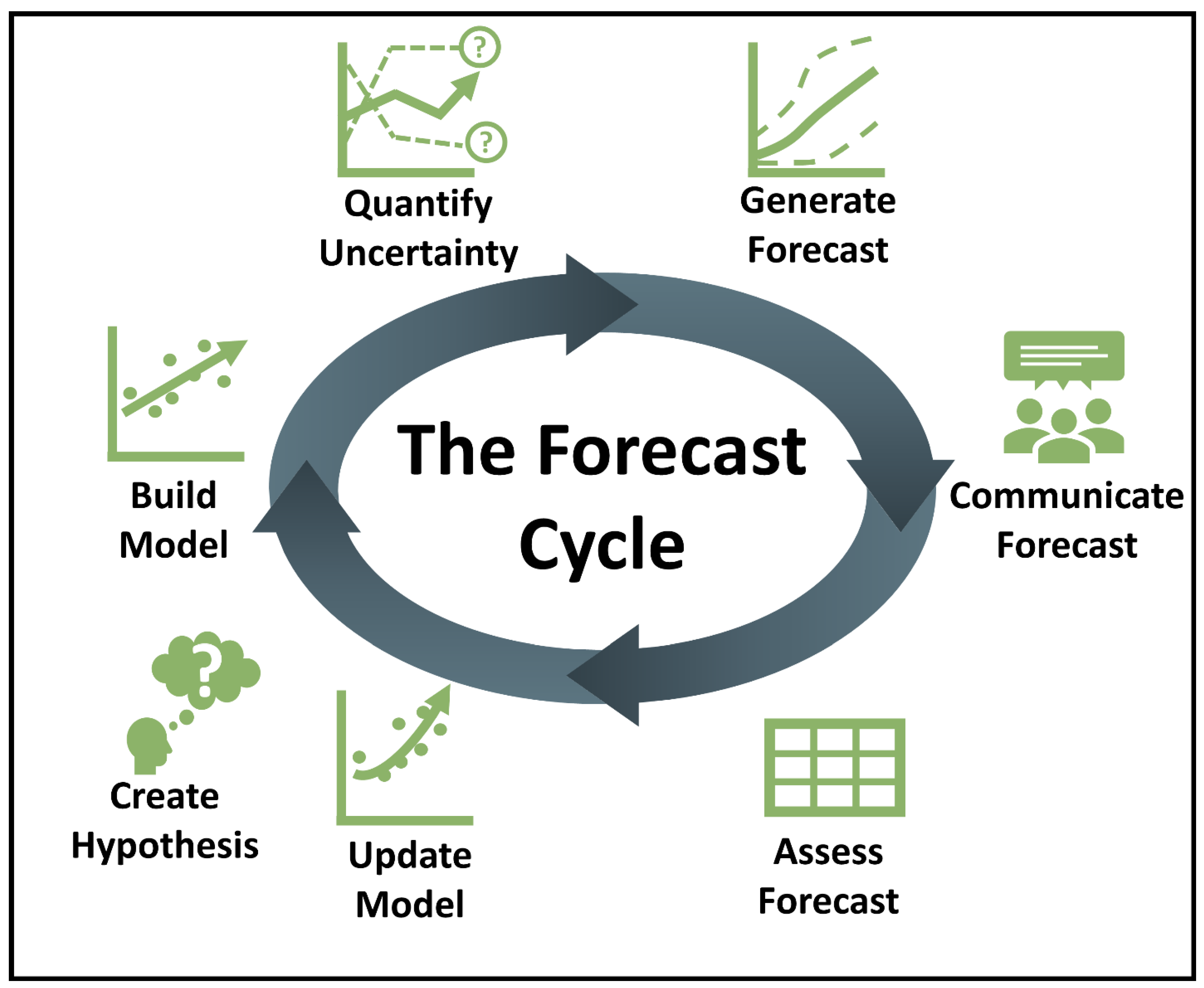
Which of the following options is a step in the iterative ecological forecast cycle?

(a) Communicating historical observations (b) Evaluating the quality of the observations (c) Updating the model with new observations (d) Reducing forecast uncertainty (e) Quantifying how often forecasts are generated

,

Table A3. Likert-type scales for student pre- and post-module self-assessment questions (Questions 1–5). This scale applied to Question 6, regarding perceived knowledge of ecological forecasting (“Select the statement below that best describes your current knowledge of ecological forecasting”), Question 7, regarding perceived knowledge of ecological forecast uncertainty (“Select the statement below that best describes your current knowledge of ecological forecast uncertainty”), and, lastly, Questions 8–10, regarding students’ perceptions of the importance of learning how to generate a forecast, quantify uncertainty, and communicate a forecast (“Using the scale below, how important do you think that the following skills are for you to learn? (a) Generating an ecological forecast; (b) Quantifying an ecological forecast’s uncertainty; (c) Communicating output from an ecological forecast”).

Metric	1	2	3	4	5
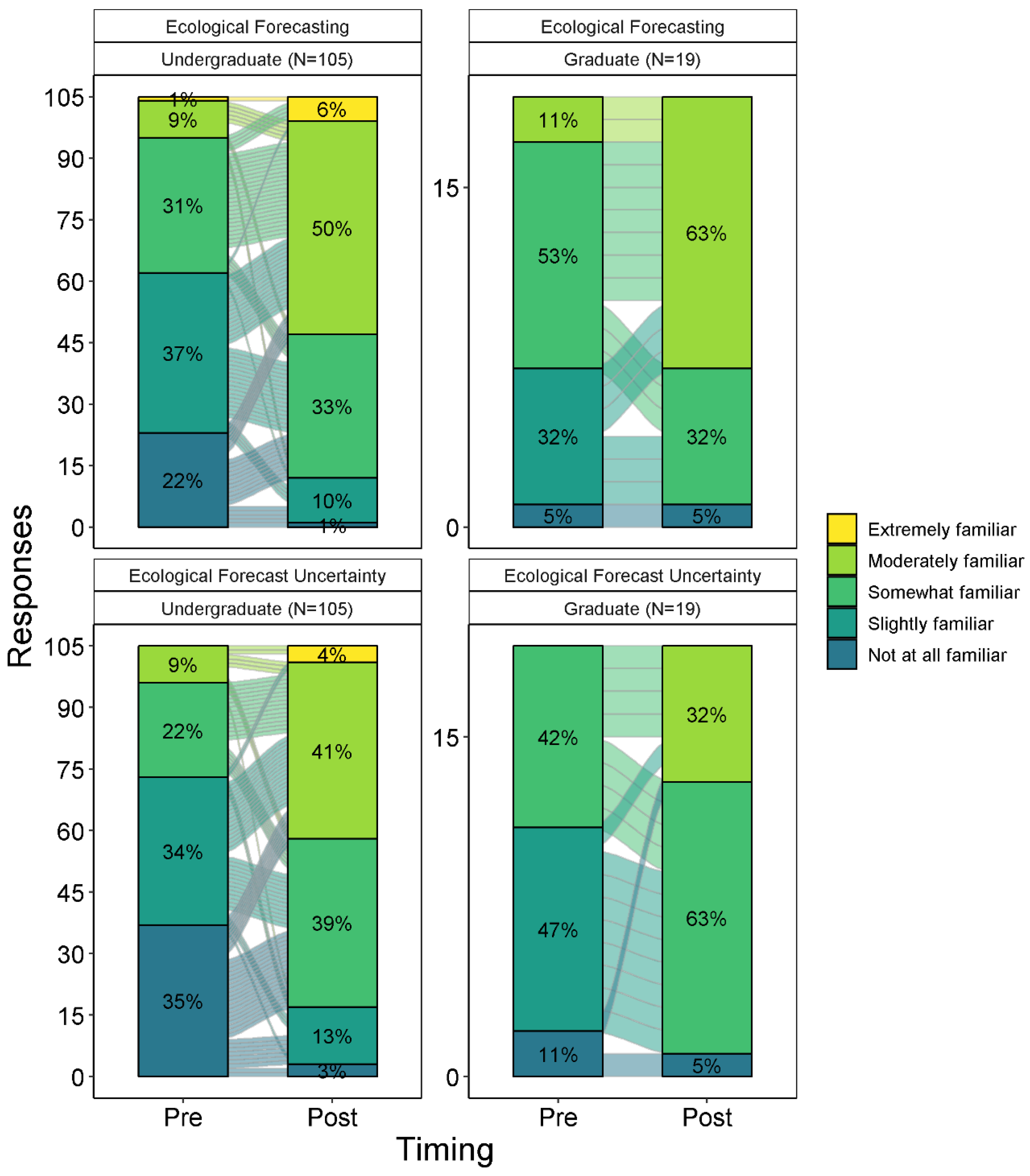
Ecological Forecasting	Not at all familiar, I have never heard of ecological forecasting.	Slightly familiar, I have heard of ecological forecasting, but cannot elaborate.	Somewhat familiar, I could explain a little about ecological forecasting.	Moderately familiar, I could explain quite a bit about ecological forecasting.	Extremely familiar, I could explain and instruct others about ecological forecasting.
Ecological Forecast Uncertainty	Not at all familiar, I have never heard of ecological forecast uncertainty.	Slightly familiar, I have heard of ecological forecast uncertainty, but cannot elaborate.	Somewhat familiar, I could explain a little about ecological forecast uncertainty.	Moderately familiar, I could explain quite a bit about ecological forecast uncertainty.	Extremely familiar, I could explain and instruct others about ecological forecast uncertainty.
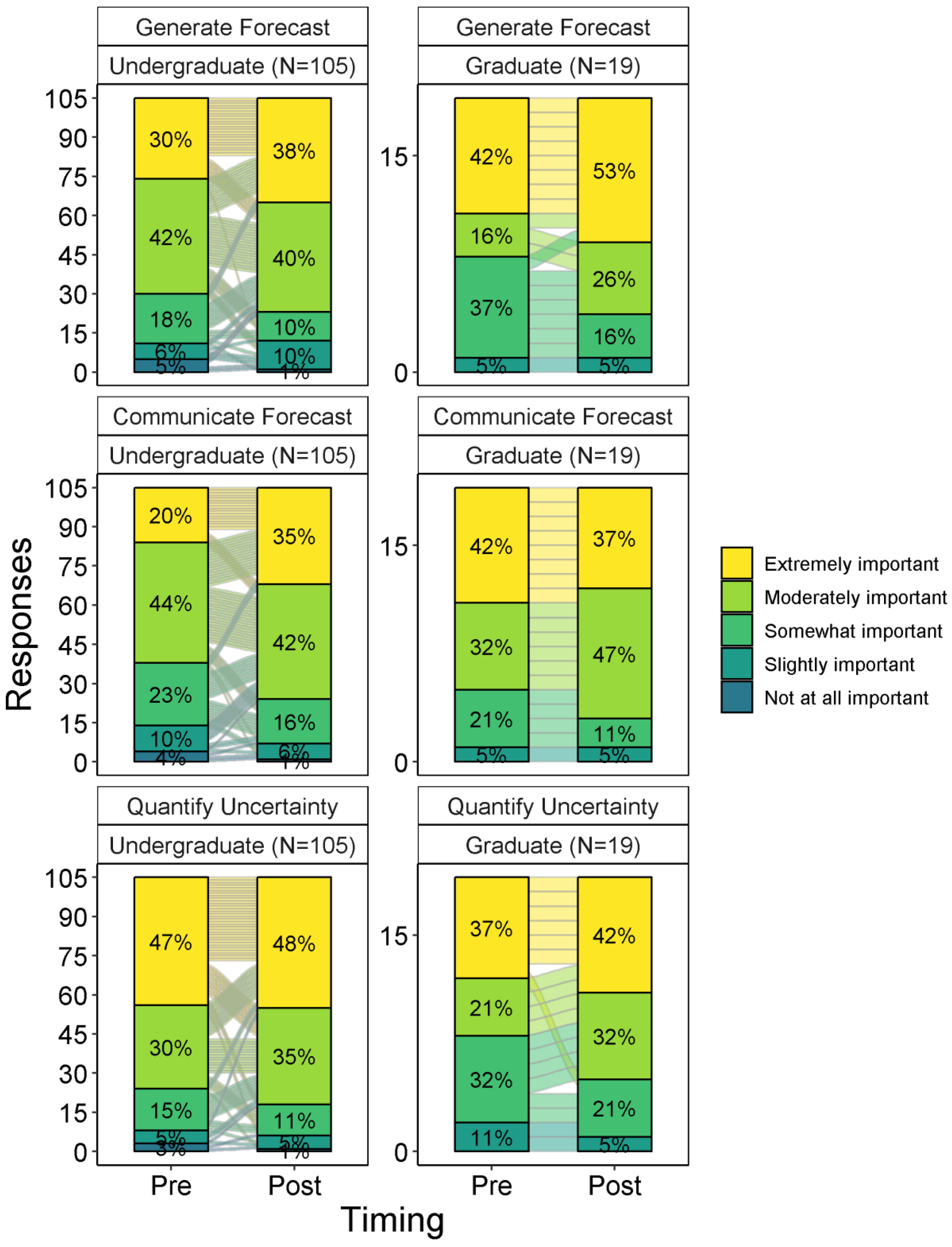
Generate Forecast; Communicate Forecast; Quantify Uncertainty	Not at all important, no need to learn	Slightly important, may be of limited use but not necessary to learn	Somewhat important, may be useful to learn	Moderately important, there is a need to learn	Very important, it is necessary to learn

and

Table A4. Free-form assessment question (Q5) for pre- and post-module responses for the module.

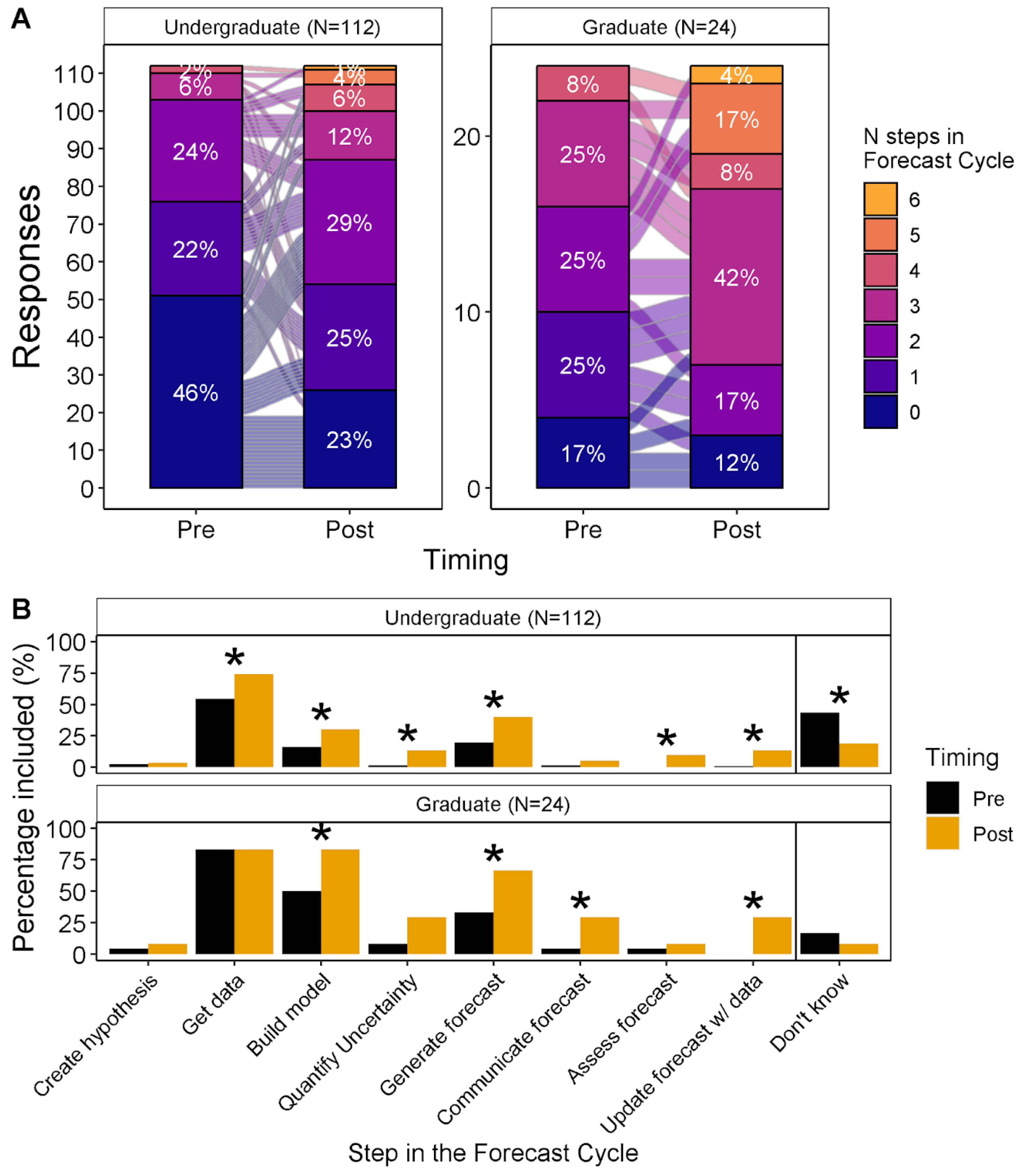
Let us pretend that you are an ecological forecaster tasked with forecasting lake algae concentrations for the next 16 days into the future to help lake managers. What steps would you propose to accomplish this goal? If you don’t know the answer, please write “I don’t know” instead of leaving the response blank.

for assessment questions). A detailed description of how qualitative questions were assessed can be found in Appendix A.1, and the description of the thematic bins used to code the students’ answers is found in

Table A5. Coding criteria used for the Q 5 thematic bins were developed using the two-step process described in S1.

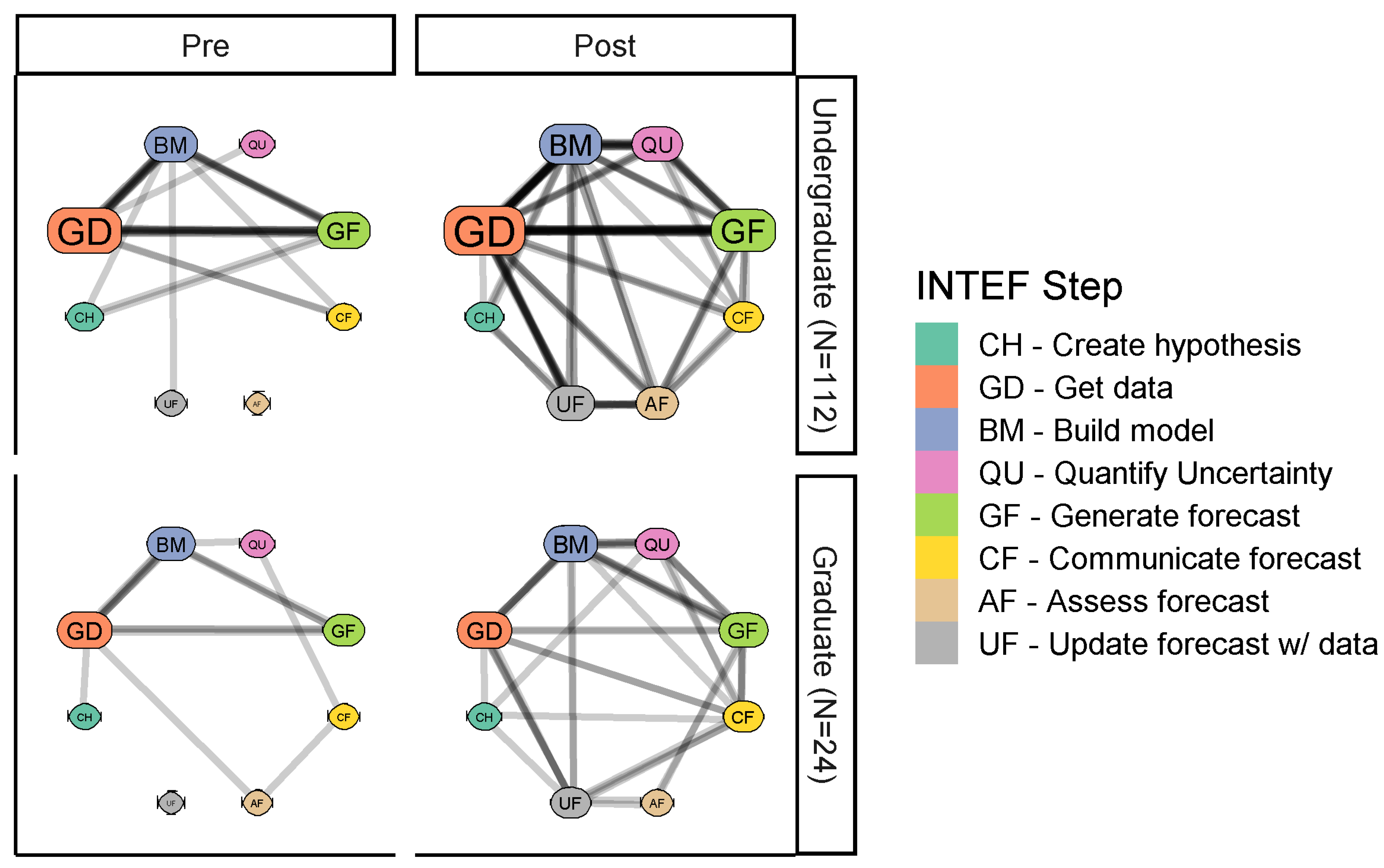
Thematic bins: Answers were scored for the presence or absence of each “bin” (create hypothesis, build model, quantify uncertainty, generate forecast, communicate forecast, assess forecast, update forecast with data, don’t know).
Create hypothesis	Create hypothesis, ask driving question
Build model	Build/construct/run/calibrate/develop/run model, any mention of model
Quantify uncertainty	Quantify/Include uncertainty, ensembles, any mention of uncertainty/certainty
Generate forecast	Generate forecast/predictions/projections
Communicate forecast	Communicate/present forecast
Assess forecast	Assess/validate forecast, compare forecast with observations, confront forecast with data
Update forecast with data	Update/readjust/recalibrate model/parameters/states/forecast with data/observations, feed data into model
Don’t know	I don’t know

.

The pre- and post-module assessments included four types of questions to assess students’ growth. First, students completed four multiple-choice questions which evaluated their ability to correctly answer questions about ecological forecasting concepts and the INTEF cycle. Second, a free-response question evaluated students’ ability to apply ecological forecasting concepts in a novel context. Students were asked: “Let us pretend that you are an ecological forecaster tasked with forecasting lake algae concentrations for the next 16 days into the future to help lake managers. What steps would you propose to accomplish this goal? If you don’t know the answer, please write ‘I don’t know’ instead of leaving the response blank.” The aim of this question was to examine how many and which steps of the INTEF cycle the students included in their responses. Third, students ranked their self-perceived knowledge of ecological forecasting and ecological forecast uncertainty on a Likert-type scale from 1 (low, “Not at all familiar”) to 5 (high, “Extremely familiar”). Finally, students completed multiple-choice questions in which they ranked their perceived importance of generating a forecast, communicating a forecast, and quantifying forecast uncertainty on a Likert-type scale from 1 (low, “Not at all important”) to 5 (high, “Very important”). The first two types of questions gave us the opportunity to quantify students’ growth in response to completing the module, whereas the latter questions allowed us to quantify students’ self-perceptions.

We analyzed the assessment data using standard methods [42,43]. For all questions, we analyzed the undergraduate student responses separately from the graduate students. We used paired Wilcoxon signed-rank tests to compare pre- and post-module responses for the multiple-choice questions as well as to compare the mean pre- and post-module Likert scores for the questions examining students’ perceived importance and knowledge of ecological forecasting. The free-response question was coded using standardized answer rubrics to classify pre- and post-module student responses, which were subsequently compared with Wilcoxon signed-rank tests (see Appendix A.1 for detailed methods and Table A4 for the answer rubric). The number of students who filled out both the pre- and post-module assessments varied for each question, resulting in differing n in the analyses. We did not have a control group to compare our results to, which was a limitation in the design of this experiment. Statistical significance was defined as p < 0.05. All analyses were completed in R version 4.1.3 [44].

Faculty who taught the modules were provided with a faculty feedback form following teaching of the module. This form asked faculty about the ease of teaching the module in their classroom and their perceptions of the module’s effectiveness at teaching ecological forecasting concepts and collected any additional feedback relating to their experience teaching the module.

All students and faculty consented to participate in the study per our Institutional Review Board (IRB) protocols (Virginia Tech IRB 19-669 and Carleton College IRB #19-20 065).

3. Results

Our assessment data indicated that completion of the module significantly increased students’ understanding of ecological forecasting concepts and ability to apply approaches of the iterative ecological forecasting cycle to novel contexts (Figure 3 and Figure 4). Moreover, students’ self-perceptions of their understanding of ecological forecasting and the importance of ecological forecasting significantly increased after completing the module, as described below.

Undergraduate students’ understanding of ecological forecasting concepts significantly increased after completion of the module, as indicated by a greater proportion of correct answers on three of the four multiple-choice, knowledge-based questions between the pre- and post-module assessment (Figure 3; all statistical results provided in

Table A7. Statistical differences in student pre- and post-module responses to the four multiple-choice, knowledge-based questions (Q1–4, described above and in text) for undergraduate (UG) and graduate (Grad) student levels. Test statistics and p-values are for paired, two-sided Wilcoxon signed-rank tests. Significant p-values (p < 0.05) are shown in bold.

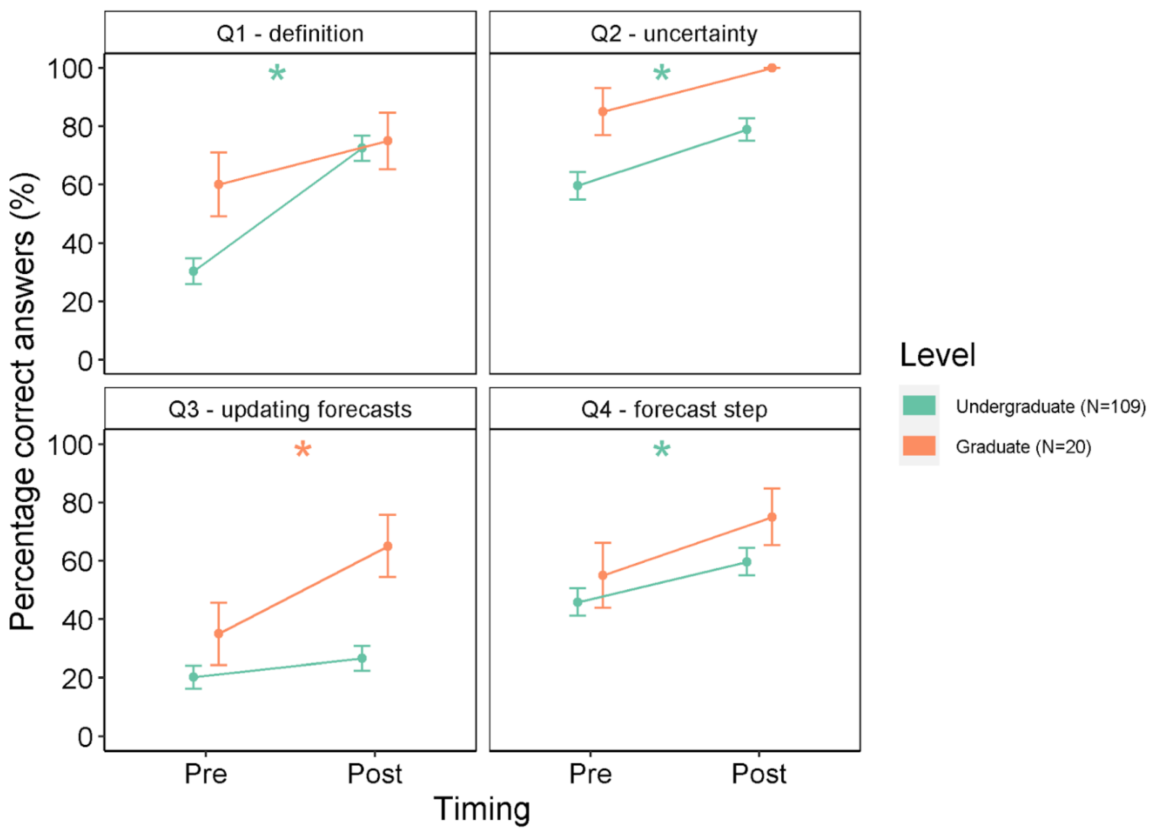
Question	Level	Test Statistic	Two-Tailed p-Value	n	Pre-Module Correct (%)	Post-Module Correct (%)	Effect Size
Q1—definition	Grad	8	0.30	20	60.0	75.0	0.23
Q1—definition	UG	110	<0.01	109	30.3	72.5	Inf
Q2—uncertainty	Grad	0	0.15	20	85.0	100.0	0.32
Q2—uncertainty	UG	152	<0.01	109	59.6	78.9	0.32
Q3—updating forecasts	Grad	4.5	0.04	20	35.0	65.0	0.46
Q3—updating forecasts	UG	192	0.21	109	20.2	26.6	0.12
Q4—forecast step	Grad	0	0.07	20	55.0	75.0	0.40
Q4—forecast step	UG	308	0.02	109	45.9	59.6	0.22

). Question 1, which asked students to define an ecological forecast, had the largest increase in the percentage of correct answers for undergraduate students, going from 30.2% pre-module to 72.5% post-module (Figure 3; Table A7). For multiple-choice Questions 2 and 4, the percentage of correct answers for undergraduates also increased significantly from pre- to post-module assessment, from 59.6% to 78.9% and 45.9% to 59.6%, respectively (Figure 3; Table A7; See Table A4 for questions).

Student experience level affected the ability to correctly answer the assessment questions, as the graduate students consistently scored higher than the undergraduate students (Figure 3). However, regardless of education level, all students showed improvement for all four questions. Interestingly, Question 3 exhibited a significant increase for graduate students, from 35% to 65%, but not for the undergraduate students, from 20.2% to 26.6%. This question asked students, “Which of the following options is NOT an advantage of iteratively updating forecasts with data over time?”

After completing the module, undergraduate students were significantly more knowledgeable about the INTEF cycle and able to apply it in a novel context (Figure 4). For the free-response question asking how they would forecast lake algae, both undergraduate and graduate students were significantly more likely to describe the use of iterative, near-term forecasting in their answer after completing the module. For example, one students’ pre-module answer was “Use historic amounts of algae and their population growth and graph it to forecast the future;” after completing the module, this student’s response was “use available data to create a model, then use the model to predict the future, then communicate it to the managers.” Another student’s pre-module answer was “…take various measurements to determine algae concentrations over the 16 days, record the data, analyze data to find trends, use a population model to predict how the population might change based on your data and the model,” whereas after the module, their response was “learn about factors that affect the lake, build a model based on past data, use the model to make predictions, and then use new data to adjust the model.”

The students’ responses indicate increased knowledge of the INTEF cycle after module completion. Specifically, undergraduates’ pre-module responses contained a median of zero INTEF steps, which increased to two steps in the post-module responses (Figure 4A; Table 2). The steps that were significantly more likely to be included in undergraduates’ responses after module completion were “get data” (54.5% to 74.1%), “build model” (16.1% to 30.4%), “generate forecast” (19.6% to 40.2%), “quantify uncertainty” (1.8% to 13.4%), and “assess forecast” (0% to 9.8%) (Figure 4B;

Table A6. Differences in the number of INTEF cycle steps included in students’ responses to Question 5, “Let us pretend that you are an ecological forecaster tasked with forecasting lake algae concentrations for the next 16 days into the future to help lake managers. What steps would you propose to accomplish this goal? If you don’t know the answer, please write ‘I don’t know’ instead of leaving the response blank” between pre- and post-module assessments for graduate (Grad) and undergraduate (UG) students. Test statistics and p-values are for paired, two-sided Wilcoxon signed-rank tests; pre- and post-module means are reported with the standard deviations (SD) along with pre- and post-module medians and the interquartile range (IQR). Significant p-values (p < 0.5) are shown in bold.

Level	Test Statistic	Two-Tailed p-Value	n	Pre-Module Mean (±1 SD)	Pre-Module Median (IQR)	Post-Module MEAN (±1 SD)	Post-Module Median (IQR)	Effect Size
Grad	10	0.001	24	1.8 ± 1.2	2 (1, 3)	3.0 ± 1.6	3 (2, 4)	0.68
UG	647.5	0.000	112	1.0 ± 1.1	1 (0, 2)	1.7 ± 1.4	2 (1, 2)	0.42

). There was a significant decrease in the number of undergraduate students who reported “I don’t know” (43.8% to 18.8%) to this question, which corresponded with an increase in the percentage of undergraduate students who included two or more steps in their response, from 32% to 52%.

While the number of steps identified in the INTEF cycle after module completion significantly increased for both undergraduate and graduate students, graduate students exhibited a larger increase overall. The forecast steps which saw the largest significant increase for graduate students following module completion were “build model” (50.0% to 83.3%), “generate forecast” (33.3% to 66.7%), “communicate forecast” (4.2% to 29.2%), and “update forecast with data” (0% to 29.2%). The steps “quantify uncertainty,” “communicate forecast,” and “update forecast with data” were generally identified at low rates for both undergraduate and graduate students, even in the post-module assessment, at <30%.

We note that some students, primarily undergraduates, did not include steps in their post-questionnaires that were included in their pre-questionnaires (

Table A9. Number of students out of the total undergraduate (UG, N = 112) and graduate student (Grad, N = 24) populations who included each step in the forecast cycle in their pre-module questionnaire but not in their post-module questionnaire.

Level	Create Hypothesis	Get Data	Build Model	Quantify Uncertainty	Generate Forecast	Communicate Forecast	Assess Forecast	Update Forecast w/Data
UG	3	7	9	1	9	2	0	0
Grad	1	2	0	1	0	0	0	0

). The steps which undergraduates were most often left out of the post-questionnaire but identified during the pre-questionnaire were: “Get data” (n = 7), “Build model” (n = 9), and “Generate forecast” (n = 9). Interestingly, these were the steps which were included at the highest percentages in the pre-module survey (54.5%, 16.1%, and 19.6%, respectively; Figure 4B). In contrast, there were very few graduate students who did not include some steps in the post-module assessment that were previously included in the pre-module assessment (Table A9).

Network analysis reveals clear differences in students’ schema of the INTEF cycle before and after completing the module (Figure 5). In the pre-module assessment, both undergraduate and graduate students’ responses were clearly anchored by the three steps of the INTEF cycle the students were most familiar with: “Get data,” “Build model, and “Generate forecast.” Noticeably, there were some steps that were not identified by any undergraduate (“Assess forecast”) and graduate students (“Update forecast”) in any of their pre-module responses.

Following completion of the module and exposure to the mental model of the INTEF cycle (Figure 1), there was an expansion in the number of steps that both undergraduate and graduate students included in their responses. For undergraduate students, the “Get data” step anchored their schema of the INTEF cycle, meaning that it was not only the step that was identified the most, but it was also most likely to influence the inclusion of other steps in their responses. The inclusion of other steps in undergraduate students’ post-module responses (especially “Build model” and “Update forecast with data”) was anchored upon the “Get data” step, as indicated by the strength of the pairwise connections. In other words, it was rare for students to include other steps in the INTEF cycle if “Get data” was absent from their responses. This pattern suggests that linking the other INTEF steps to “Get data” more explicitly in future instruction could be an effective approach for scaffolding the INTEF cycle steps for undergraduates, vs. focusing on the INTEF cycle as a whole.

In contrast, graduate students’ post-module responses were much more likely to have an even distribution of pairwise connections, suggesting that their schema of the INTEF cycle was less focused on one particular node and, instead, the complete cycle. The evenness among edges may indicate a higher level of systems thinking in understanding the INTEF cycle, but the lower number of graduate students in the assessment necessitates additional data collection for exploring this pattern further. Across both student populations, all of the INTEF steps were included in the post-module assessment, although the steps “Create hypothesis,” “Communicate forecast,” and “Assess forecast” were included by only a small number of students for both undergraduates and graduates.

Students’ self-perceptions of their knowledge of ecological forecasting and ecological forecast uncertainty showed significant increases from the pre- to post-assessment for both undergraduates and graduates (Figure 6). For undergraduate students, the increase in the five-point Likert scale went from a mean of 2.3 (“slightly familiar”) to 3.5 (“moderately familiar”) when describing their self-perceptions of their knowledge of ecological forecasting and 2.0 (“slightly familiar”) to 3.3 (“moderately familiar”) for quantifying ecological uncertainty (Figure 6;

Table A10. Differences in students’ self-reported familiarity with ecological forecasting and ecological forecast uncertainty between pre- and post-module assessments for graduate (Grad) and undergraduate (UG) level of students. Test statistics and p-values are for paired, two-sided Wilcoxon signed-rank tests; pre- and post-module means are reported with the standard deviations (SD) along with pre- and post-module medians and the interquartile range (IQR). Significant p-values (p < 0.05) are shown in bold. Questions used a Likert-type scale from 1 (low) to 5 (high) (S2).

Skill	Level	Test Statistic	Two-Tailed p-Value	n	Pre-Module Mean (±1 SD)	Pre-Module Median (IQR)	Post-Module Mean (±1 SD)	Post-Module Median (IQR)	Effect Size
Ecological Forecasting	Grad	0	<0.01	19	2.7 ± 0.7	3 (2, 3)	3.5 ± 0.8	4 (3, 4)	0.76
Ecological Forecasting	UG	201	<0.01	105	2.3 ± 0.9	2 (2, 3)	3.5 ± 0.8	4 (3, 4)	0.74
Ecological Forecast Uncertainty	Grad	0	<0.01	19	2.3 ± 0.7	2 (2, 3)	3.2 ± 0.7	3 (3, 4)	0.81
Ecological Forecast Uncertainty	UG	216	<0.01	105	2.0 ± 1.0	2 (1, 3)	3.3 ± 0.9	3 (3, 4)	0.74

). Graduate students had similar shifts in their post-module assessments, with mean increases from 2.7 (“slightly familiar”) to 3.5 (“moderately familiar”) for their knowledge of ecological forecasting. Interestingly, both undergraduate and graduate students ranked the importance of the skills of generating an ecological forecast, communicating an ecological forecast, and quantifying ecological forecast uncertainty as “moderately important” or “extremely important” on both the pre- and post-module assessment (>50%) (Figure 7;

Table A11. Differences in students’ self-reported assessment of the importance of generating a forecast, communicating a forecast, and quantifying uncertainty between pre- and post-module assessments for graduate (Grad) and undergraduate (UG) level of students. Test statistics and p-values are for paired, two-sided Wilcoxon signed-rank tests; pre- and post-module means are reported with the standard deviations (SD) along with pre- and post-module medians and the interquartile range (IQR). Significant p-values (p < 0.05) are shown in bold. Questions used a Likert-type scale from 1 (low) to 5 (high) (S2).

Skill	Level	Test Statistic	Two-Tailed p-Value	n	Pre-Module Mean (±1 SD)	Pre-Module Median (IQR)	Post-Module Mean (±1 SD)	Post-Module Median (IQR)	Effect Size
Generate Forecast	Grad	0.0	0.05	19	3.9 ± 1.0	4 (3,5)	4.3 ± 0.9	5 (4,5)	0.45
Generate Forecast	UG	653.5	0.10	105	3.9 ± 1.1	4 (3,5)	4.0 ± 1.0	4 (4,5)	0.16
Communicate Forecast	Grad	2.0	0.77	19	4.1 ± 0.9	4 (3.5,5)	4.2 ± 0.8	4 (4,5)	0.07
Communicate Forecast	UG	402.0	<0.01	105	3.7 ± 1.0	4 (3,4)	4.0 ± 0.9	4 (4,5)	0.38
Quantify Uncertainty	Grad	8.0	0.15	19	3.8 ± 1.1	4 (3,5)	4.1 ± 0.9	4 (3.5,5)	0.33
Quantify Uncertainty	UG	676.5	0.30	105	4.1 ± 1.0	4 (4,5)	4.2 ± 0.9	4 (4,5)	0.10

).

4. Discussion

In this study, our assessment data suggest that ecological forecasting can successfully be integrated into undergraduate ecology curricula and improve students’ understanding of ecological forecasting. After completing the short (3-h) “Introduction to Ecological Forecasting” module, students were significantly more likely to describe how iterative, near-term ecological forecasting could be used to generate forecasts in a new context, as well as identify steps from the INTEF cycle when designing a forecast system. The module also increased student’s familiarity with ecological forecasts and ecological forecast uncertainty, and significantly improved their ability to define an ecological forecast. In sum, these assessment data support that students were successfully able to accomplish the module’s five learning outcomes.

Importantly, the assessment data show that undergraduate students can grasp complex ecological concepts and computational skills, such as data exploration and inquiry, data visualization, ecological modeling, and quantitative reasoning, and retain the information within a laboratory or course period. Undergraduate students’ self-perceptions of familiarity with INTEF (Figure 7) and demonstrated understanding of INTEF concepts both significantly increased, highlighting that the learning objectives are aligned with how students perceive their own growth. Given the significant investment in time and expertise required for instructors to build their own quantitative inquiry-based lessons [23], our module fills an existing gap in the accessibility of materials available for instructors to easily integrate ecological forecasting concepts into undergraduate classrooms.

This module is based on training students on the entire INTEF cycle within one class period. Our approach was to teach the entire INTEF cycle together at a high level, rather than breaking the INTEF into multiple separate lessons. We found that teaching the entire cycle together allowed students to feel self-accomplishment about completing the INTEF cycle. This was reflected in some of the faculty feedback we collected: “I think the emphasis on iterative forecasting worked well psychologically: After the module, they were all talking to each other about what they would do on their next round of model improvement. The chance to improve the model is compelling and addictive.” Showing the students all the steps motivated them to understand the overall importance of INTEF as an approach.

During the initial development of the module, we implemented the module in two classrooms not included in the assessment and received feedback from both instructors and students on ways to iteratively improve the materials. For example, in an earlier version of the module, students were tasked with calibrating the ecological model to measurements of total nitrogen and chlorophyll-a in Activity A. Instructors reported that fitting two variables for the model was confusing for students, so we then removed total nitrogen and instead had students solely focus on fitting chlorophyll-a. This early feedback likely led to a more engaging and effective teaching module for both students and instructors and, following the INTEF cycle, ensures that the module is also iteratively improved with data.

Teaching the entire INTEF cycle in one lesson is also associated with some challenges. For example, it is possible that the reason why some INTEF steps (e.g., “quantify uncertainty,” “communicate forecast,” and “update forecast with data”) did not exhibit significant increases from the pre- to post-module answers to the free-response question (Figure 4) was because some of the ecological content was outside the scope of the class. For example, the NP model and aquatic primary productivity may have been new material for general ecology students. This was reflected in the faculty feedback: “The ecological content didn’t match our course as well as I hoped, but using the tool was a great experience for our students!” Student retention of all the INTEF steps may also have been limited by covering all seven INTEF steps in 3 h. The module may have introduced too many new concepts to students, limiting their ability to identify some of the steps which were less intuitive or less familiar (e.g., communicate forecast, update forecast, forecast uncertainty).

Interestingly, there was a decrease in the identification of some forecast steps in the post-module questionnaire that had previously been included in the pre-module questionnaire by some undergraduates (Table A9). This change may have been related to teaching the entire INTEF cycle in one lesson. We hypothesize that the steps which were not included by students in the post-module responses may have been concepts which students were more likely to have familiarity with before completing the module (e.g., “Get data,” “Build model,” “Generate forecast”). Following completion of the module, students were more likely to identify new INTEF steps such as “Communicate forecast,” “Assess forecast,” and “Update forecast with data,” which they likely were previously less familiar with, indicating that they were focusing primarily on new content without integrating it into their prior knowledge. Altogether, this finding suggests that the module could potentially be teaching too much new information within one lesson for novice students. Either breaking the module into smaller chunks (e.g., teaching Activity A, B, and C separately) or having students complete complimentary INTEF modules in addition to this one could help to reinforce these concepts and scaffold their knowledge gains more effectively.

Data from NEON are a valuable resource for ecological forecasting education. The use of real-world examples and real ecological data allows students to relate to a sense of place, making the module content much more relevant to students [45]. Our teaching module adds to the growing number of teaching resources which are using NEON data [46], though it is the first, to the best of our knowledge, to use NEON data for teaching forecasting to undergraduates. Moreover, our module can be taught using different modalities (hybrid, virtual, in-person), which provides a flexible approach for integrating NEON data into ecology curricula [47].

Our study shows that R shiny applications can be a particularly useful mechanism for integrating ecological forecasting into undergraduate classrooms for several reasons. First, active learning approaches such as web applets and interactive software such as R Shiny applications have been shown to be a useful tool for increasing diverse representation within science [48]. Second, our work suggests that R Shiny applications are a promising methodology for overcoming potential pitfalls to teaching complex topics, such as ecological forecasting, to undergraduates. This was reflected in faculty feedback: “The addition of the Shiny app definitely streamlined the data analysis process and allowed the students to focus more on the concepts than on the mechanics of the analysis.” For ecological forecasting specifically, the R Shiny interactive platform provided a way to reduce the intimidation barrier to the INTEF cycle that is usually associated with learning ecological modeling and computer programming languages. Third, the R programming language is one of the most common languages for data analysis, with >50% of recent publications in ecology citing R in their methods [49]. Given this increasing prevalence, using R Shiny in our module provides a potential approach for instructors to adapt their own data analysis in R code into an R Shiny application without having to teach students the R programming language. Similarly, instructors could build students’ introductory programming skills by teaching a concept or lesson through an R Shiny application and then subsequently introducing students to the underlying R Shiny code to introduce them to R programming. For future development of this lesson, an accompanying Rmarkdown document would allow for further scaffolding of this lesson, especially for more advanced students. Overall, similar to our study, R Shiny applications have shown great potential in other educational contexts for improving the student learning experience and engaging them directly in the subject matter [32,34].

Our study provides several potential directions for future education research on ecological forecasting, especially at the undergraduate level. First, our study included data from only one module with a focus on teaching the entire INTEF cycle. The depth and scope of this emerging field necessitates additional modules alongside this one to complement and reinforce some of the key concepts, as indicated by the finding that some steps of the INTEF cycle were less likely to be identified after module completion, despite all being equally taught in the module. Developing further educational materials on the steps in the INTEF cycle which students were less likely to include in their answers (Figure 4B), such as quantifying uncertainty, communicating ecological forecasts, and updating forecasts with data, in greater depth will, overall, increase students’ knowledge and consolidate these concepts for undergraduate and graduate students (Figure 4B). It has been shown that completing multiple inquiry-based courses can consolidate this learning [50]. Second, we had differing numbers of students per class, which prevented us from doing a substantive analysis of how differences in module modality, student experience level, and course type affected module effectiveness. Due to the imbalance in numbers of undergraduate versus graduate students, the inferences we can draw from our analysis of the effects of module completion on graduate students’ growth is limited. Third, we further note that our experimental design, which compared pre-module vs. post-module responses, was limited by not having a control group of students. Finally, our student assessment timeline was limited to completing the post-module questions up to two weeks after the module. Ideally, an additional, longer-term assessment would provide better insights into knowledge retention by students.

This module, “Introduction to Ecological Forecasting,” likely in parallel with others which cover the topics of quantifying uncertainty, data assimilation, and communicating forecasts in greater depth, will help educate, prepare, and train the next generation of ecological forecasters. Moreover, an integrated module curriculum paves the way for embedding and incorporating data science principles into undergraduate ecological education more broadly. Given the increasing need for ecological forecasting in the face of more variable environmental conditions due to global change, we anticipate that the need for ecological forecasting education will only grow over time. In response, our module and others can serve a valuable role for preparing undergraduates for future data-rich careers by providing them with a foundational perspective that they can build skills on.

References

- Carey, C.C.; Woelmer, W.M.; Lofton, M.E.; Figueiredo, R.J.; Bookout, B.J.; Corrigan, R.S.; Daneshmand, V.; Hounshell, A.G.; Howard, D.W.; Lewis, A.S.L.; et al. Advancing Lake and Reservoir Water Quality Management with Near-Term, Iterative Ecological Forecasting. Inland Waters 2022, 12, 107–120. [Google Scholar] [CrossRef]
- Dietze, M.C.; Fox, A.; Beck-Johnson, L.M.; Betancourt, J.L.; Hooten, M.B.; Jarnevich, C.S.; Keitt, T.H.; Kenney, M.A.; Laney, C.M.; Larsen, L.G.; et al. Iterative Near-Term Ecological Forecasting: Needs, Opportunities, and Challenges. Proc. Natl. Acad. Sci. USA 2018, 115, 1424–1432. [Google Scholar] [CrossRef] [PubMed] [Green Version]
- Tulloch, A.I.T.; Hagger, V.; Greenville, A.C. Ecological Forecasts to Inform Near-Term Management of Threats to Biodiversity. Glob. Chang. Biol. 2020, 26, 5816–5828. [Google Scholar] [CrossRef]
- White, E.P.; Yenni, G.M.; Taylor, S.D.; Christensen, E.M.; Bledsoe, E.K.; Simonis, J.L.; Ernest, S.K.M. Developing an Automated Iterative Near-Term Forecasting System for an Ecological Study. Methods Ecol. Evol. 2019, 10, 332–344. [Google Scholar] [CrossRef] [Green Version]
- Woelmer, W.M.; Bradley, L.M.; Haber, L.T.; Klinges, D.H.; Lewis, A.S.L.; Mohr, E.J.; Torrens, C.L.; Wheeler, K.I.; Willson, A.M. Ten Simple Rules for Training Yourself in an Emerging Field. PLoS Comput. Biol. 2021, 17, e1009440. [Google Scholar] [CrossRef] [PubMed]
- Lewis, A.S.L.; Woelmer, W.M.; Wander, H.L.; Howard, D.W.; Smith, J.W.; McClure, R.P.; Lofton, M.E.; Hammond, N.W.; Corrigan, R.S.; Thomas, R.Q.; et al. Increased Adoption of Best Practices in Ecological Forecasting Enables Comparisons of Forecastability. Ecol. Appl. 2022, 32, e2500. [Google Scholar] [CrossRef] [PubMed]
- Bever, A.J.; Friedrichs, M.A.M.; St-Laurent, P. Real-Time Environmental Forecasts of the Chesapeake Bay: Model Setup, Improvements, and Online Visualization. Environ. Model. Softw. 2021, 140, 105036. [Google Scholar] [CrossRef]
- Record, N.R.; Pershing, A.J. Facing the Forecaster’s Dilemma: Reflexivity in Ocean System Forecasting. Oceans 2021, 2, 738–751. [Google Scholar] [CrossRef]
- Scavia, D.; Bertani, I.; Testa, J.M.; Bever, A.J.; Blomquist, J.D.; Friedrichs, M.A.M.; Linker, L.C.; Michael, B.D.; Murphy, R.R.; Shenk, G.W. Advancing Estuarine Ecological Forecasts: Seasonal Hypoxia in Chesapeake Bay. Ecol. Appl. 2021, 31, e02384. [Google Scholar] [CrossRef]
- Thomas, R.Q.; Figueiredo, R.J.; Daneshmand, V.; Bookout, B.J.; Puckett, L.K.; Carey, C.C. A Near-Term Iterative Forecasting System Successfully Predicts Reservoir Hydrodynamics and Partitions Uncertainty in Real Time. Water Resour. Res. 2020, 56, e2019WR026138. [Google Scholar] [CrossRef]
- Dietze, M.C. Ecological Forecasting; Princeton University Press: Princeton, NJ, USA, 2017; ISBN 978-1-4008-8545-9. [Google Scholar]
- Dietze, M.C.; Lynch, H. Forecasting a Bright Future for Ecology. Front. Ecol. Environ. 2019, 17, 3. [Google Scholar] [CrossRef]
- Bodner, K.; Rauen Firkowski, C.; Bennett, J.R.; Brookson, C.; Dietze, M.; Green, S.; Hughes, J.; Kerr, J.; Kunegel-Lion, M.; Leroux, S.J.; et al. Bridging the Divide between Ecological Forecasts and Environmental Decision Making. Ecosphere 2021, 12, e03869. [Google Scholar] [CrossRef]
- Greengrove, C.; Lichtenwalner, C.S.; Palevsky, H.I.; Pfeiffer-Herbert, A.; Severmann, S.; Soule, D.; Murphy, S.; Smith, L.M.; Yarincik, K. Using Authentic Data from NSF’s Ocean Observatories Initiative in Undergraduate Teaching. Oceanography 2020, 33, 62–73. [Google Scholar] [CrossRef]
- Kjelvik, M.K.; Schultheis, E.H. Getting Messy with Authentic Data: Exploring the Potential of Using Data from Scientific Research to Support Student Data Literacy. CBE Life Sci. Educ. 2019, 18, es2. [Google Scholar] [CrossRef] [PubMed]
- O’Reilly, C.M.; Gougis, R.D.; Klug, J.L.; Carey, C.C.; Richardson, D.C.; Bader, N.E.; Soule, D.C.; Castendyk, D.; Meixner, T.; Stomberg, J.; et al. Using Large Data Sets for Open-Ended Inquiry in Undergraduate Science Classrooms. BioScience 2017, 67, 1052–1061. [Google Scholar] [CrossRef] [Green Version]
- Burrow, A.K. Teaching Introductory Ecology with Problem-Based Learning. Bull. Ecol. Soc. Am. 2018, 99, 137–150. [Google Scholar] [CrossRef] [Green Version]
- Rieley, M. Big Data Adds up to Opportunities in Math Careers: Beyond the Numbers; Bureau of Labor Statistics: Washington, DC, USA, 2018. [Google Scholar]
- FACT SHEET: President Biden Takes Executive Actions to Tackle the Climate Crisis at Home and Abroad, Create Jobs, and Restore Scientific Integrity Across Federal Government. Available online: https://www.whitehouse.gov/briefing-room/statements-releases/2021/01/27/fact-sheet-president-biden-takes-executive-actions-to-tackle-the-climate-crisis-at-home-and-abroad-create-jobs-and-restore-scientific-integrity-across-federal-government/ (accessed on 15 November 2021).
- Carey, C.C.; Farrell, K.J.; Hounshell, A.G.; O’Connell, K. Macrosystems EDDIE Teaching Modules Significantly Increase Ecology Students’ Proficiency and Confidence Working with Ecosystem Models and Use of Systems Thinking. Ecol. Evol. 2020, 10, 12515–12527. [Google Scholar] [CrossRef]
- Sormunen, M.; Heikkilä, A.; Salminen, L.; Vauhkonen, A.; Saaranen, T. Learning Outcomes of Digital Learning Interventions in Higher Education: A Scoping Review. CIN: Comput. Inform. Nurs. 2022, 40, 154–164. [Google Scholar] [CrossRef]
- Subhash, S.; Cudney, E.A. Gamified Learning in Higher Education: A Systematic Review of the Literature. Comput. Hum. Behav. 2018, 87, 192–206. [Google Scholar] [CrossRef]
- Auker, L.A.; Barthelmess, E.L. Teaching R in the Undergraduate Ecology Classroom: Approaches, Lessons Learned, and Recommendations. Ecosphere 2020, 11, e03060. [Google Scholar] [CrossRef] [Green Version]
- Carey, C.C.; Gougis, R.D. Simulation Modeling of Lakes in Undergraduate and Graduate Classrooms Increases Comprehension of Climate Change Concepts and Experience with Computational Tools. J. Sci. Educ. Technol. 2017, 26, 1–11. [Google Scholar] [CrossRef] [Green Version]
- Chang, W.; Cheng, J.; Allaire, J.J.; Sievert, C.; Schloerke, B.; Xie, Y.; Allen, J.; McPherson, J.; Dipert, A.; Borges, B. Shiny: Web Application Framework for R. 2021. Available online: https://cran.r-project.org/web/packages/shiny/index.html (accessed on 25 April 2022).
- Zhu, M.; Johnson, M.; Dutta, A.; Panorkou, N.; Samanthula, B.; Lal, P.; Wang, W. Educational Simulation Design to Transform Learning in Earth and Environmental Sciences. In Proceedings of the 2020 IEEE Frontiers in Education Conference (FIE), Uppsala, Sweden, 21–24 October 2020; pp. 1–6. [Google Scholar]
- Derkach, T.M. The Origin of Misconceptions in Inorganic Chemistry and Their Correction by Computer Modelling. J. Phys. Conf. Ser. 2021, 1840, 012012. [Google Scholar] [CrossRef]
- Biehler, R.; Fleischer, Y. Introducing Students to Machine Learning with Decision Trees Using CODAP and Jupyter Notebooks. Teach. Stat. 2021, 43, S133–S142. [Google Scholar] [CrossRef]
- Hayyu, A.N.; Dafik; Tirta, I.M.; Wangguway, Y.; Kurniawati, S. The Analysis of the Implementation Inquiry Based Learning to Improve Student Mathematical Proving Skills in Solving Dominating Metric Dimention Number. J. Phys. Conf. Ser. 2020, 1538, 012093. [Google Scholar] [CrossRef]
- Williams, I.J.; Williams, K.K. Using an R Shiny to Enhance the Learning Experience of Confidence Intervals. Teach. Stat. 2018, 40, 24–28. [Google Scholar] [CrossRef]
- Kasprzak, P.; Mitchell, L.; Kravchuk, O.; Timmins, A. Six Years of Shiny in Research—Collaborative Development of Web Tools in R. R J. 2020, 12, 155. [Google Scholar] [CrossRef]
- Fawcett, L. Using Interactive Shiny Applications to Facilitate Research-Informed Learning and Teaching. J. Stat. Educ. 2018, 26, 2–16. [Google Scholar] [CrossRef] [Green Version]
- González, J.A.; López, M.; Cobo, E.; Cortés, J. Assessing Shiny Apps through Student Feedback: Recommendations from a Qualitative Study. Comput. Appl. Eng. Educ. 2018, 26, 1813–1824. [Google Scholar] [CrossRef]
- Neyhart, J.L.; Watkins, E. An Active Learning Tool for Quantitative Genetics Instruction Using R and Shiny. Nat. Sci. Educ. 2020, 49, e20026. [Google Scholar] [CrossRef]
- Moore, T.N.; Carey, C.C.; Thomas, R.Q. Macrosystems EDDIE Module 5: Introduction to Ecological Forecasting (Instructor Materials). 2022. [CrossRef]
- Prevost, L.; Sorensen, A.E.; Doherty, J.H.; Ebert-May, D.; Pohlad, B. 4DEE—What’s Next? Designing Instruction and Assessing Student Learning. Bull. Ecol. Soc. Am. 2019, 100, e01552. [Google Scholar] [CrossRef]
- Carey, C.C.; Darner Gougis, R.; Klug, J.L.; O’Reilly, C.M.; Richardson, D.C. A Model for Using Environmental Data-Driven Inquiry and Exploration to Teach Limnology to Undergraduates. Limnol. Oceanogr. Bull. 2015, 24, 32–35. [Google Scholar] [CrossRef] [Green Version]
- Bybee, R.W.; Taylor, J.A.; Gardner, A.; Van Scotter, P.; Carlson Powell, J.; Westbrook, A.; Landes, N. The BSCS 5E Instructional Model: Origins and Effectiveness; Colorado Springs, Co: Colorado Springs, CO, USA, 2006. [Google Scholar]
- Soetaert, K.; Herman, P.M.J. Model Formulation. In A Practical Guide to Ecological Modelling: Using R as a Simulation Platform; Springer: Dordrecht, The Netherlands, 2009; pp. 15–69. ISBN 978-1-4020-8624-3. [Google Scholar]
- Jolliffe, I.T.; Stephenson, D.B. Forecast Verification a Practitioner’s Guide in Atmospheric Science, 2nd ed.; Wiley-Blackwell: Chichester, UK, 2012. [Google Scholar]
- Moore, T.N.; Carey, C.C.; Thomas, R.Q. Macrosystems EDDIE Module 5: Introduction to Ecological Forecasting (R Shiny Application); Zenodo: Geneva, Switzerland, 2022. [Google Scholar] [CrossRef]
- Miles, M.B.; Huberman, A.M.; Saldaña, J. (Eds.) Qualitative Data Analysis: A Methods Sourcebook, 3rd ed.; SAGE Publications, Inc.: Thousand Oaks, CA, USA, 2014; ISBN 978-1-4522-5787-7. [Google Scholar]
- Vogt, W.P. Dictionary of Statistics & Methodology: A Nontechnical Guide for the Social Sciences, 3rd ed.; Sage Publications: Thousand Oaks, CA, USA, 2005; ISBN 978-0-7619-8854-0. [Google Scholar]
- R Core Team. R: A Language and Environment for Statistical Computing; R Foundation for Statistical Computing: Vienna, Austria, 2022. [Google Scholar]
- Cid, C.R.; Pouyat, R.V. Making Ecology Relevant to Decision Making: The Human-Centered, Place-Based Approach. Front. Ecol. Environ. 2013, 11, 447–448. [Google Scholar] [CrossRef]
- Nagy, R.C.; Balch, J.K.; Bissell, E.K.; Cattau, M.E.; Glenn, N.F.; Halpern, B.S.; Ilangakoon, N.; Johnson, B.; Joseph, M.B.; Marconi, S.; et al. Harnessing the NEON Data Revolution to Advance Open Environmental Science with a Diverse and Data-Capable Community. Ecosphere 2021, 12, e03833. [Google Scholar] [CrossRef]
- Record, S.; Jarzyna, M.A.; Hardiman, B.; Richardson, A.D. Open Data Facilitate Resilience in Science during the COVID-19 Pandemic. Front. Ecol. Environ. 2022, 20, 76–77. [Google Scholar] [CrossRef]
- Ballen, C.J.; Wieman, C.; Salehi, S.; Searle, J.B.; Zamudio, K.R. Enhancing Diversity in Undergraduate Science: Self-Efficacy Drives Performance Gains with Active Learning. CBE Life Sci. Educ. 2017, 16, ar56. [Google Scholar] [CrossRef]
- Lai, J.; Lortie, C.J.; Muenchen, R.A.; Yang, J.; Ma, K. Evaluating the Popularity of R in Ecology. Ecosphere 2019, 10, e02567. [Google Scholar] [CrossRef] [Green Version]
- Beck, C.W.; Blumer, L.S. Inquiry-Based Ecology Laboratory Courses Improve Student Confidence and Scientific Reasoning Skills. Ecosphere 2012, 3, art112. [Google Scholar] [CrossRef]