Article

High-Resolution Gridded Air Temperature Data for the Urban Environment: The Milan Data Set

Fondazione Osservatorio Meteorologico Milano Duomo, I-20145 Milano, Italy
*
Author to whom correspondence should be addressed.
Forecasting 2022, 4(1), 238-261; https://doi.org/10.3390/forecast4010014
Submission received: 29 December 2021 / Revised: 27 January 2022 / Accepted: 4 February 2022 / Published: 8 February 2022
(This article belongs to the Special Issue Surface Temperature Forecasting)

Abstract

:
Temperature is the most used meteorological variable for a large number of applications in urban resilience planning, but direct measurements using traditional sensors are not affordable at the usually required spatial density. On the other hand, spaceborne remote sensing provides surface temperatures at medium to high spatial resolutions, almost compatible with the needed requirements. However, in this case, limitations are represented by cloud conditions and passing times together with the fact that surface temperature is not directly comparable to air temperature. Various methodologies are possible to take benefits from both measurements and analysis methods, such as direct assimilation in numerical models, multivariate analysis, or statistical interpolation. High-resolution thermal fields in the urban environment are also obtained by numerical modelling. Several codes have been developed to resolve at some level or to parameterize the complex urban boundary layer and are used for research and applications. Downscaling techniques from global or regional models offer another possibility. In the Milan metropolitan area, given the availability of both a high-quality urban meteorological network and spaceborne land surface temperatures, and also modelling and downscaling products, these methods can be directly compared. In this paper, the comparison is performed using: the ClimaMi Project high-quality data set with the accurately selected measurements in the Milan urban canopy layer, interpolated by a cokriging technique with remote-sensed land surface temperatures to enhance spatial resolution; the UrbClim downscaled data from the reanalysis data set ERA5; a set of near-surface temperatures produced by some WRF outputs with the building environment parameterization urban scheme. The comparison with UrbClim and WRF of the cokriging interpolated data set, mainly based on the urban canopy layer measurements and covering several years, is presented and discussed in this article. This comparison emphasizes the primary relevance of surface urban measurements and highlights discrepancies with the urban modelling data sets.

1. Introduction

In the current climate change situation, cities represent one of the most relevant environments, mainly because a large percentage of human population lives in urbanized areas: more than 56% already in 2020, with a still growing trend and a projection up to 68% in 2050 (United Nations Department of Economic and Social Affairs—Population Dynamics: World Urbanization Prospects 2018 (https://population.un.org/wup/), last accessed on 7 January 2022). Therefore, large quantities of energy and pollution are produced, which exacerbate the well-known urban heat island (UHI) phenomenon and severely affect inhabitant wellness. This is especially true during heat wave (HW) episodes [1], when UHI adds its effect to the already-elevated temperatures caused by the synoptic weather situation. Nevertheless, UHI has several diversified aspects, depending on regional climate, topographic characteristics, urban shape, and urban metabolism. It is then clear that a good observational knowledge of urban meteorology and climatology is an essential part of every effort in urban resilience plans worldwide.
On the other hand, atmospheric processes in the urban atmosphere are difficult to handle, essentially because they are dominated by turbulence of the more complex boundary layer and by the large gradients of surface characteristics. Both aspects imply the necessity of meteorological high-resolution spatial and temporal observations, land use and land cover details, and specific complex modelling techniques. A general review of all these items is given in [2].
In cities, near-surface meteorological measurements are affected by a number of unavoidable disturbances. Therefore, they usually hardly meet the WMO (World Meteorological Organization (https://public.wmo.int/), last accessed on 10 January 2022) requirements for correct (meso-) synoptic measurements [3]. Thus, in most cases classification for urban meteorological sensors is in WMO Class 4 or more often Class 5 with the largest estimated uncertainties, while classical climatological stations must be in Class 1. Nevertheless, it must be noted that in cities the observational target is the local- and microscale characterization of the urban atmosphere, as affected by nearby buildings and other urbanistic features. Therefore, even if classified in WMO Class 5 where the temperature uncertainties are estimated to be up to 5 °C, they are necessary, and the WMO specifies this need with the suffix “s” (i.e., “special”): specific cautions must be taken into consideration for correct and representative measurements. Technical and methodological requirements are given by [4], where particular attention is paid to siting and sensor exposure: the former is intended as the station position relative to the main urban characteristics and boroughs (urban mesoscale), the latter as the exact location of each sensor relative to nearby disturbing details as shadows and reflections, radiating walls, greeneries, parks, aquifers, and so on. Both aspects are an essential part of the measurement representativeness.
The relevance of UHI effects on both energy production and human wellness makes temperature the most important among all the meteorological essential climatic variables (ECVs) (ECVs are defined by GCOS: https://gcos.wmo.int/en/essential-climate-variables, last accessed on 10 January 2022). For urban applications, especially in adaptation and mitigation plans, temperature is needed by local authorities and engineering and architectural professionals at a spatial resolution comparable to boroughs and single buildings or building blocks (i.e., at the order of a few tenths of meters and even less) [5]. Furthermore, it must be stressed that also vertical gradients are relevant because of the 3D nature of urbanized environments [2]: meteorological and climatological measurement targets are different if sensors are at street level, in parks, or at building tops. They must be considered separately regarding different layers of the urban atmosphere. Even their representativeness is different, as well as their potential applications: measurements at street level are more directly related to human wellness, but their horizontal representativeness is very limited. On the other hand, measuring at building top level (the upper part of the urban canopy layer (UCL)) produces data that are representative of a larger area and requires much fewer measuring points for a satisfactory description of the city: in this case, applications are obviously quite different. It is also evident that detailed metadata of the observational network stations, relating to both siting and exposure, are of utmost relevance. Well-planned (in terms of urban layer, siting, and exposure), well-managed (in terms of calibration and maintenance procedures), and well-described meteorological networks (metadata) can then produce climatological data with much lower uncertainties [6]. Evidently, the sustainability of the measuring network is a major problem too, especially considering long-lasting applications and climatological purposes. Even considering the opportunities recently offered by low-cost sensors and Internet of Things solutions, the observational requirements depending on spatial resolution are hardly to be met, for both logistical and economical aspects: it is not always easy to find a suitable and practicable location for sensors, and their quantity must be limited to a reasonable number.
Classical near-surface measurements can be integrated by remote-sensed data: in situ measuring points are necessarily limited in number, while remote sensing allows for monitoring a large area with a generally elevated spatial resolution. Moreover, spaceborne sensors are becoming more and more frequent, and their data are often easily accessible. In this case, the observational frequency is poor, severely limited by orbital characteristics of the orbiting platforms: in the best case, no more than one or two measurements per day are possible, and often repetition occurs after several days. In the specific case of temperature measurements, one other aspect is relevant. The temperature range at the earth surface limits measurements in the thermal infrared (IR) around the 10 μm wavelength, where radiation is strongly absorbed only by condensed water, and around the maximum of the radiation intensity emitted by the earth surface. Therefore, only situations without clouds are practically open to remote sensing of temperature from space. Furthermore, the radiation sensed comes essentially from the earth surface: the derived temperature is then the land surface temperature (LST), not directly comparable to the near-surface air temperature (Ta), measured “in situ”. LST computation needs a lot of auxiliary variables, and different methods have been described [7]: LST data are directly provided for a few spaceborne observational platforms too. There are several ways to take advantage of both air temperature direct measurements and remote-sensed LST. In general, the results are in the form of gridded fields of temperature at a resolution depending mainly on the resolution of LST data, typically about 102 ÷ 103 m, with possible downscaling at lower values.
Modelling of the urban atmosphere is obviously another way to obtain air temperature fields in cities. Much work has been done with two different approaches: considering the impact of single buildings or building blocks on an initially undisturbed environment and developing an atmospheric model nesting and improving the resolution down to building dimensions. In the former case, very high resolutions are achievable [8,9], but mesoscale meteorological dynamics is often underestimated; in the latter, very high resolutions are more difficult to obtain [10]. Modelling, however, requires observational data to be properly initialized for both sensitivity analysis and results verification.
In this paper, we focus on the assessment of urban air temperature fields, achieved by integrating high-quality near-surface measurements with high-resolution remote-sensed LSTs in Milan and the surrounding area. The integration methodology adopted is based on a cokriging technique (CoK) [11] and was described in a previous article [12], where direct correlations between near-surface air temperatures and LST, inverse distance weights, and ordinary kriging have also been considered and discussed. As a consequent continuation of that work, in the present paper the computed gridded fields of air temperature in the UCL and the related uncertainties are compared with other available temperature data sets based on reanalysis downscaling and with some urban modelling results. A summary of the temperature data set obtained for Milan and the adopted CoK methodology is shortly described in Section 2. Section 3 analyzes the results of the UrbClim (climate variables for cities in Europe from 2008 to 2017 (https://cds.climate.copernicus.eu/), last accessed on 10 January 2022) (in the following: UrC) air temperature data set based on a downscaling of ERA5 (ECMWF Reanalysis v5 (https://www.ecmwf.int/en/forecasts/dataset/ecmwf-reanalysis-v5), last accessed on 13 December 2021); also, some outputs of WRF model runs for the same area are compared. The overall results are then shortly discussed in Section 4, highlighting discrepancies between models and observations. Finally, in Section 5 conclusions are summarized and further developments outlined.

2. Materials and Methods

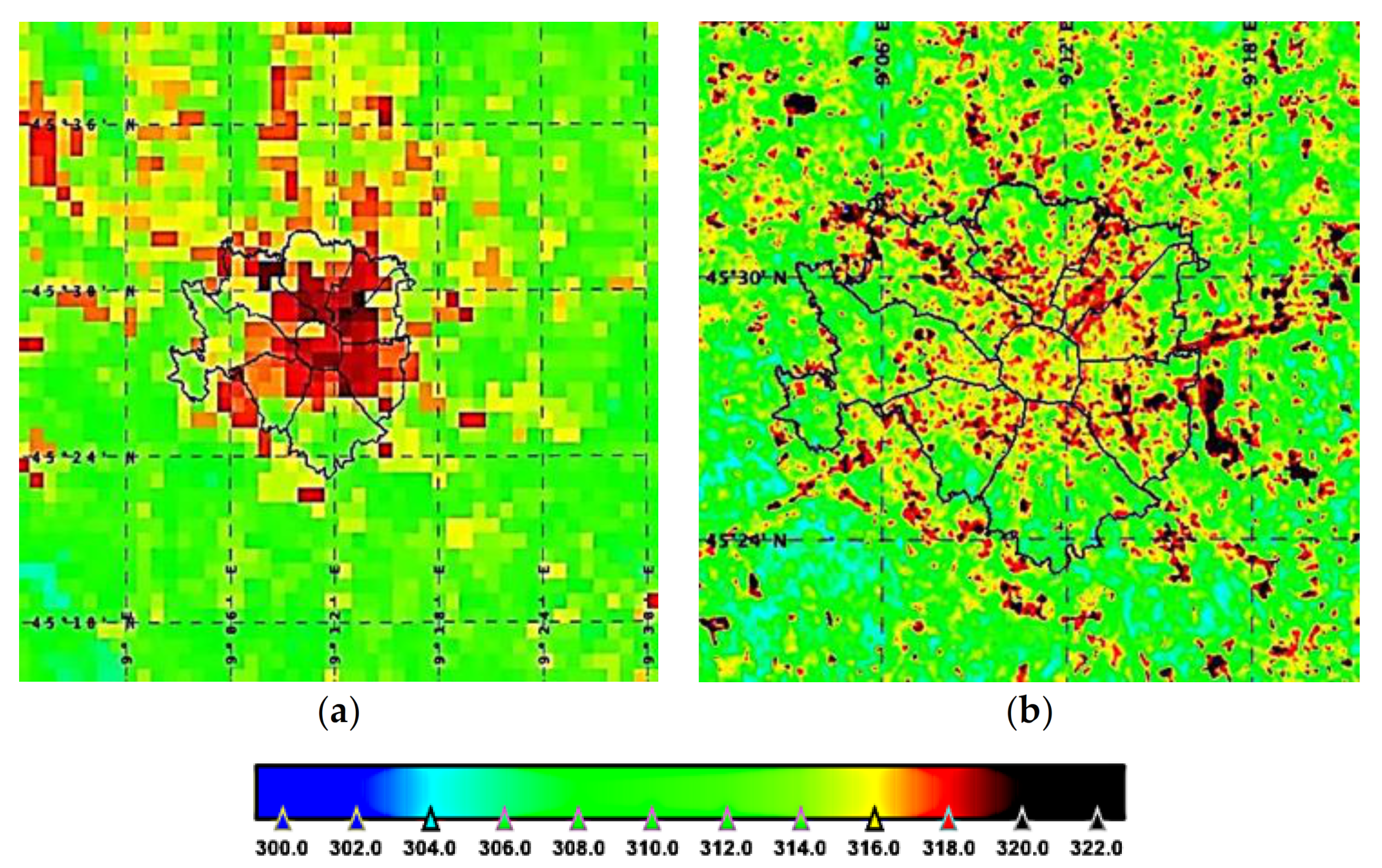
2.1. Improving the Observational Air Temperature Resolution

A realistic and affordable urban meteorological network has a number of measurement points of the order of a few tens and has a typical density of 1 station per 10 km2. This is enough to resolve the urbanized environment at the urban mesoscale, for instance, to outline the UHI morphology and dynamics. However, it is obviously inadequate for a more detailed description at the building and building-block scale. Moreover, the observational target must be specified, and the network layout must be coherently set up. For an urban mesoscale characterization, the upper part of the UCL is a reasonable solution, while for a more detailed monitoring, also the lower UCL should be considered as in the case of urban squares, green areas, and parks or aquifers inside the city, according to the local climatic zone (LCZ) classification [13].
Several cities are nowadays monitored by such networks [14,15]. In Milan, the weather network of Fondazione OMD (Fondazione Osservatorio Meteorologico Milano Duomo (https://www.fondazioneomd.it/), last accessed on 10 January 2022) Network), specifically designed for urban applications and climatological purposes [16], has been operating continuously for a decade and has so far collected a database of minima, maxima, and mean values over 10 min and of the most relevant ECVs: it consists of about 20 automatic weather stations (AWSs) distributed in the larger metropolitan area (1575 km2), 8 AWSs sited in Milan downtown (50 km2). The FOMD Network monitors the weather variables at the roof level of buildings (upper UCL), it is managed with metrological criteria and calibrated with high-quality international standards, and it is characterized by total homogeneity of AWS siting and of hardware and software [17]. Laboratory and in-field measurement uncertainties have also been evaluated [18]. The Milan FOMD subnet has allowed, therefore, a much-improved description of Milan UHI relative to previous studies [19,20].
The FOMD Network database, limited to 2016–2019 and short-time periods in 2014 and 2015, is used as the basic reference for the urban air temperature Ta. The city of Milan (Figure 1) has an almost center-symmetric configuration, covering an area of 181.8 km2 with a population of 1.4 million (2020) and a relatively high density of 7.7 × 10³ km−2. The city center is at latitude 45° 28′ N and longitude 9° 11.5′ E in the central–western part of the flat valley of Po River in Northern Italy, with the Alps northwards and westwards, the Apennines to the south, and a smooth and small elevation gradient oriented from the higher (140 m above mean sea level) northern–northwestern region to the lowland in the south–southeast. The larger metropolitan area (1575 km2 and 3.3 × 10⁶ inhabitants) has a mixed composition of smaller towns and industrial and agricultural lands, and it extends from the more than 250 m elevated region in the northwest to the less than 60 m a.m.s.l. plane in the southeast.
The FOMD Network is suitable for a description of the weather and climate in the Milan metropolitan area. However, it is not dense enough to represent in detail the temperature at the urban microscale, as required by public administrators and professionals in a number of applications, such as urban planning, energy, and building design. Therefore, we accurately selected and added to the analysis further operational weather stations managed by the Regional Environmental Protection Agency (ARPA Lombardia (Lombardy Regional Environmental Protection Agency [https://www.arpalombardia.it/Pages/Meteorologia/Osservazioni-e-Dati/Dati-in-tempo-reale.aspx]), last accessed on 13 December 2021) and by a citizen–scientist weather observers’ association (MeteoNetwork (https://www.meteonetwork.it/rete/livemap/), last accessed on 13 December 2021), connected with similar associations abroad and actively collaborating with academic and research institutions. Selection criteria were based on operational continuity, data reliability (we performed an accurate independent validation based on automatic checking and cross-reference), and siting characterization. Figure 1 gives a synoptic view of the resulting overall network, and Table 1 lists coordinates and altitudes above mean sea level of the AWSs.
Figure 1. Domain and weather stations: (a) the whole network with stations from FOMD (red), ARPA Lombardia (violet), and MeteoNetwork (orange); (b) Milan in the central part of the western Po Valley. The domain area is shown in red, equivalent to the area in (a).
Forecasting 04 00014 g001
There are different possibilities to integrate the classical “in situ” measurements with remote-sensed data from spaceborne platforms, which provide thermal IR observations at a resolution varying from 1 km to a few tens of a meter. The satellite data considered for this study were the land surface temperatures (LSTs) directly provided by ESA (European Space Agency (https://www.esa.int/Applications/Observing_the_Earth), last accessed on 13 December 2021) in the framework of the EU Copernicus (Copernicus (https://www.copernicus.eu/), last accessed on 13 December 2021) initiative, based mainly on operational measurements by Sentinels 3A and 3B, and LST data by NOAA (National Oceanic and Atmospheric Administration (https://www.noaa.gov/), last accessed on 13 December 2021) and USGS (United States Geological Survey (https://earthexplorer.usgs.gov/), last accessed on 13 December 2021), based mainly on Landsat 8 sensors. Correlation, kriging, and cokriging interpolation methods were tested using Ta and LST data for the Milan area, and their results were compared, as already described in [12]. Correlation between Ta and LST was found to be not sufficiently performing from a meteorological/physical point of view for monitoring and climatological purposes, being relatively good in some cases but practically absent in others. Best results were obtained with kriging and cokriging interpolation methods. The cokriging method (CoK), implemented on a regular grid of square cells of 100 m side that cover the metropolitan area of Milan, proved to be particularly suitable. It allows us to “model” the interpolation of AWSs’ Ta according to the LST of each square cell.
The methodology finally adopted is based on the cokriging technique [21,22]: the reference Ta was taken as the primary variable, and the satellites’ LST as the secondary one. The CoK interpolation, obtained after best fitting of the semivariograms and minimizing the covariances, generated a gridded air temperature field at the higher resolution of the secondary variable LST, but keeping a good part of the characteristics and quality of the primary one (i.e., measurements of Ta at the top of UCL). We also performed a statistical estimation of the interpolation uncertainty: in all the analyzed situations, we obtained a statistical uncertainty well under 2 °C and in most cases under 1 °C. Interpolation uncertainty is comparable with the AWSs’ Ta uncertainties due to calibration, siting, and exposure of sensors and to maintenance procedures. Specific development and application of this cokriging methodology to the Milan area and the FOMD Network database are detailed in [12].
The results, mainly obtained in the framework of ClimaMi Project (https://www.progettoclimami.it, last accessed on 10 January 2022), are medium- to high-resolution gridded fields of air temperature together with the related uncertainties, available for weather situations without clouds at the passing times of the used orbital platforms, in the morning hours (around 9:00 or 10:00 UTC) or in the evening (22:00 or 23:00 UTC). They refer to UHI and HW episodes generally occurring with anticyclonic and clear weather, at high spatial resolution for urbanistic planning, energy, and building design: both are relevant in Milan. UHI produces temperature differences, “urban–rural”, which in the annual mean are of the order of 4 °C and have maxima up to 10 °C. HW episodes are generally due to a persistent northward extension of the African subtropical high, and they are not infrequent: the annual mean of HW days (i.e., with daily temperature maxima over 33 ÷ 34 °C and minima over 23 ÷ 24 °C and lasting at least 2 days) is well over 10 in downtown.
The above-quoted resolution and uncertainty of the gridded fields are compatible with the requirements by architects and engineers resulting from collaboration with professional associations in the ClimaMi Project. Regular updates are foreseen.

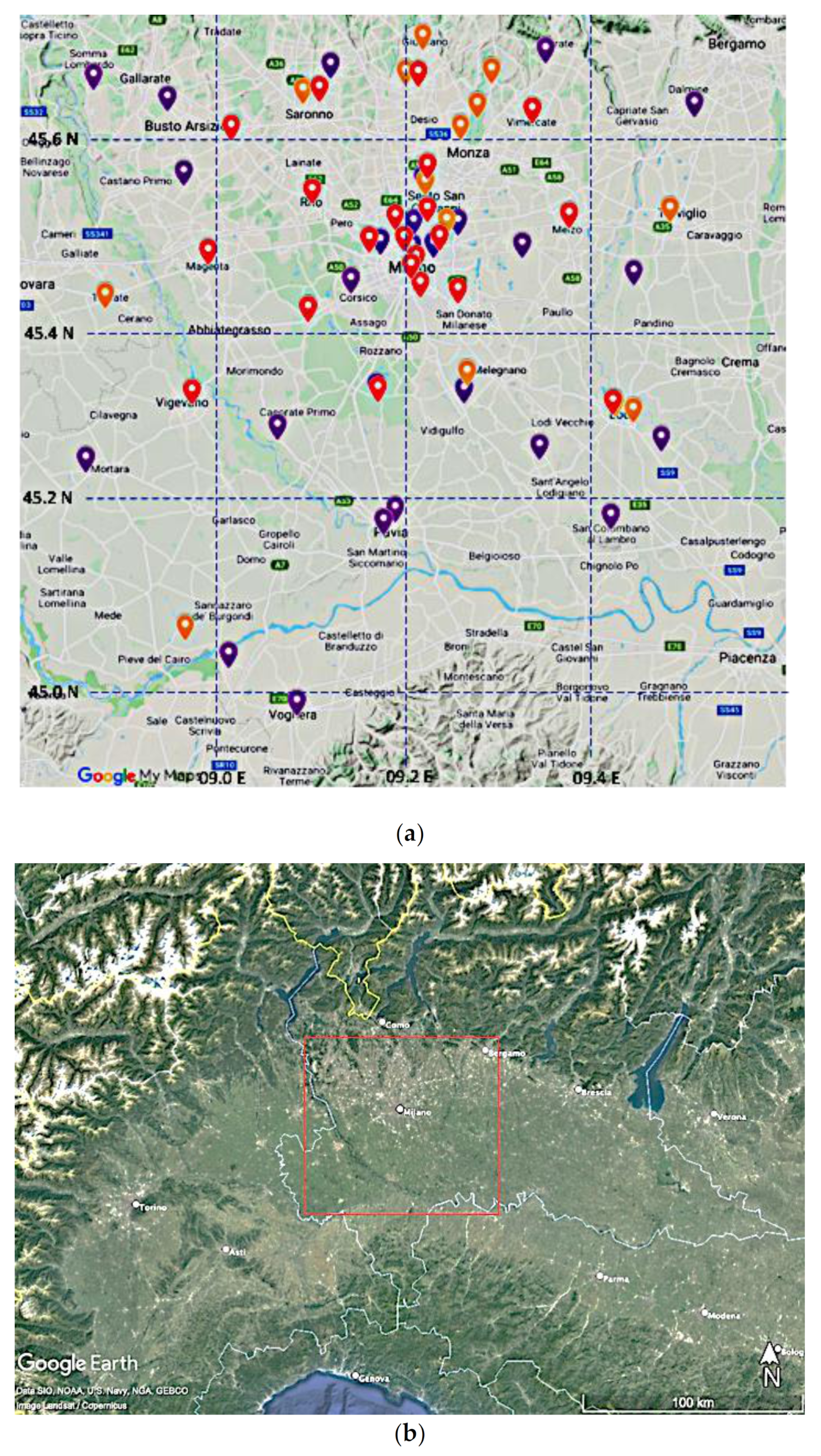
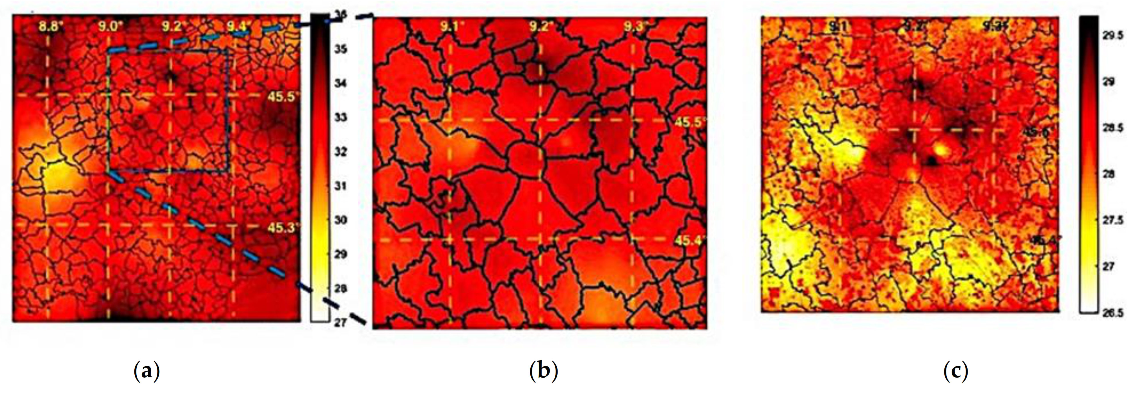
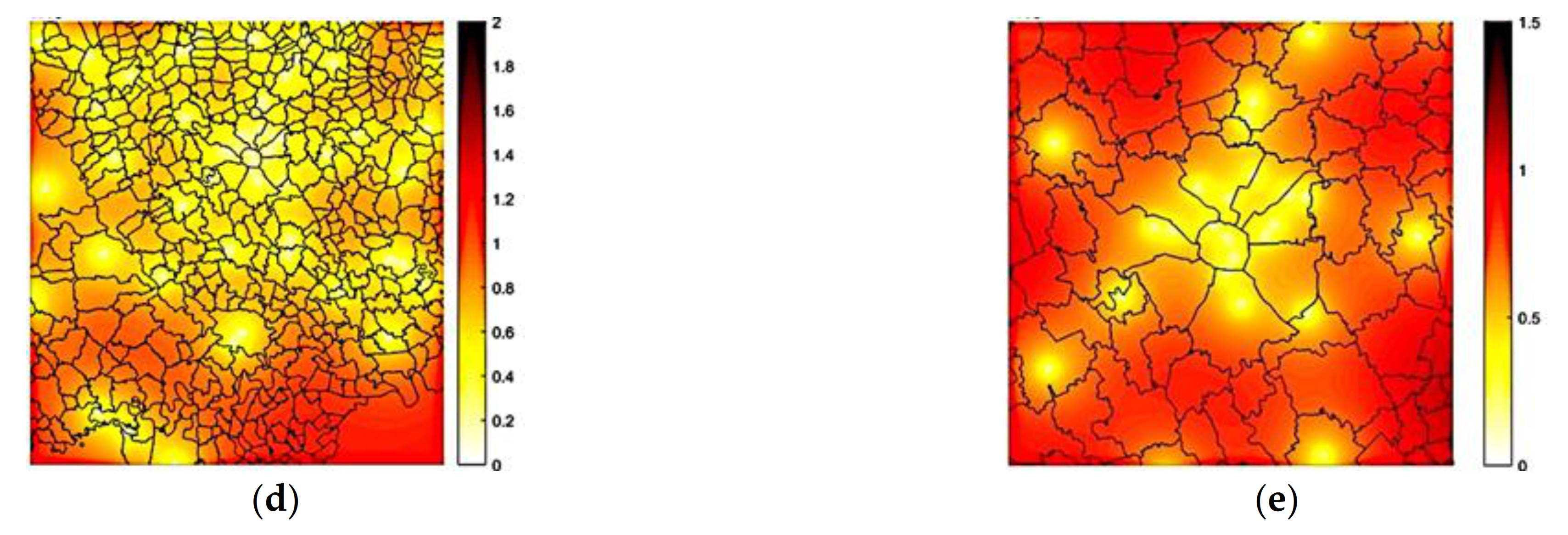
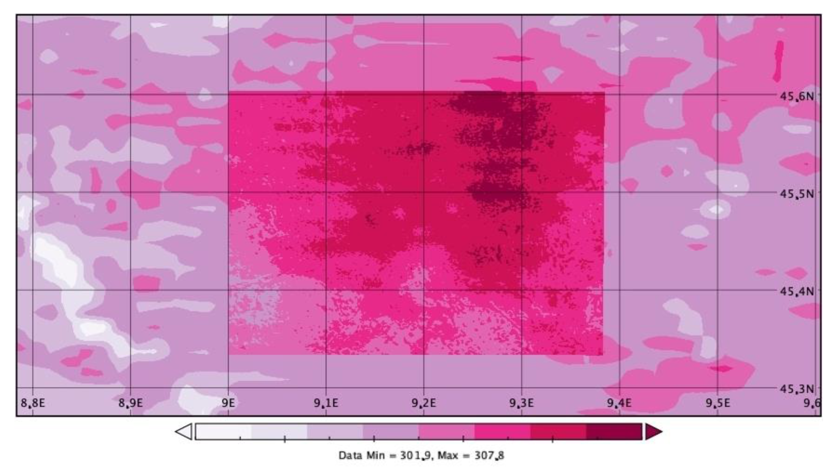
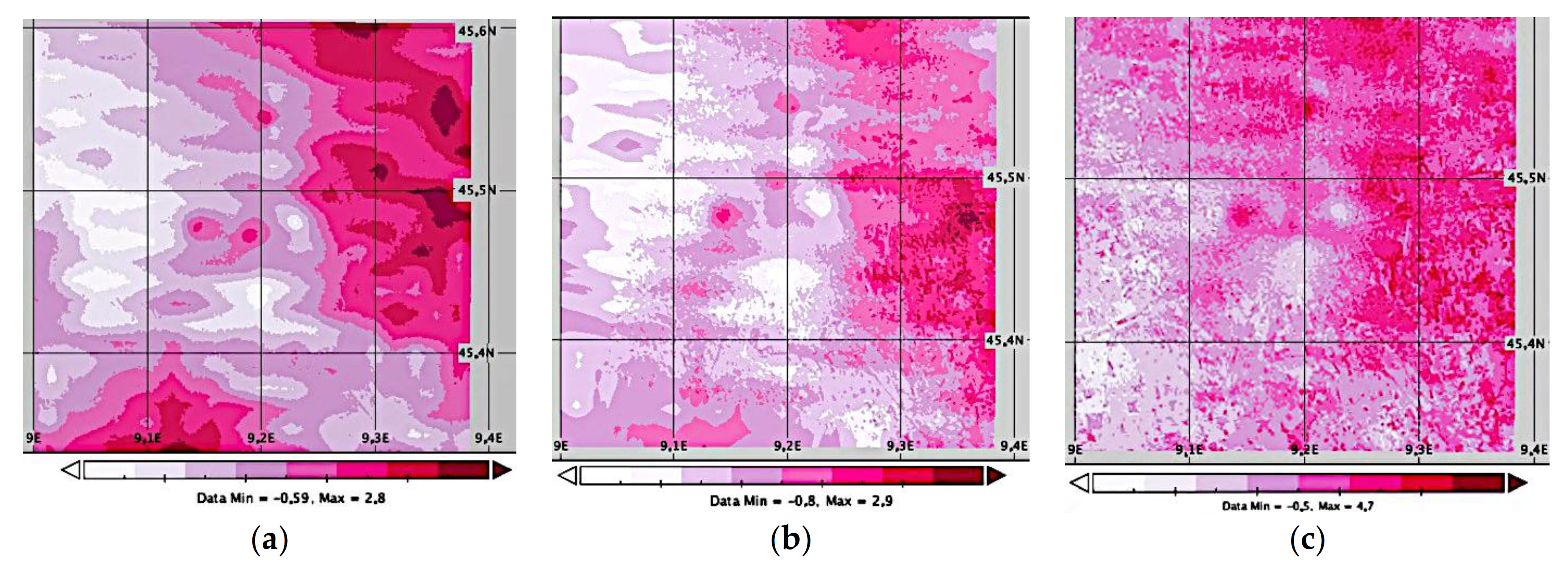
2.2. Data Set of Gridded Air Temperatures for Milan Metropolitan Area

The construction of the Milan gridded temperature database related to two different sources of information, as already previously depicted:
  • The surface meteorological database, composed of 10 min mean values obtained by:
    21 AWSs of the FOMD Network;
    26 AWSs of the institutional regional network managed by ARPA Lombardia;
    14 stations of the MeteoNetwork.
Overall, 61 stations were used. In the last two cases, an accurate selection of stations and the subsequent data validation were performed to maintain the high-quality standards as in the first one.
b.
The LST database, created by the selection of cloud-free spaceborne observations of the Milan area by two different operational platforms:
Sentinels 3A and 3B, managed by ESA under the EU Copernicus initiative, with a good repetition interval of 2 days and a medium spatial resolution of 1 km (Figure 2a);
Landsat 8, operated by NOAA and USGS with slower repetition but a much better resolution of 30 m (Figure 2b).
Figure 2. Examples of land surface temperatures (LST, K) in the Milan area from (a) Sentinel 3, 1 July 2019 09:51 UTC, at 1 km resolution and (b) Landsat 8, 1 July 2019 10:11 UTC, at 30 m resolution; color scale of LST in K. The gain in resolved details is evident in (b). Coordinates are WGS84. Milan neighborhood borders are indicated for reference.
Forecasting 04 00014 g002
The reasons for selecting these satellite sources excluding other possibilities were based on easy access to the provider’s databases, observational repetition, data quality, and spatial resolution. In a future development, this data set could be extended to other existing or planned spaceborne sensors.
Application of the specifically developed CoK algorithm produced grids of near-surface air temperatures at spatial resolutions of 100 and 30 m (Table 2): the lower (100 m, 2 satellite passes per day) suitable for climatological analysis at urban mesoscale phenomena as the UHI, and the higher (30 m, 1 morning satellite pass every 14 days) to be used for a detailed description of the thermal characteristics of the urbanized environment at the local and microscale as the post operam assessment of the microclimatic performance of urban changes at the scale of a square or a street. Examples are shown in Figure 3 together with their error maps.
Furthermore, in both resolution cases the obtained gridded thermal fields were classified on the basis of the seasonal morphological aspect of the UHI, as modified by local weather circulations. Table 3 gives a simplified overview of UHI patterns and thermal characteristics of the local weather types with respective frequencies of occurrence. Each thermal field also has its own uncertainty field: uncertainties are in the range of 2 °C, when far from AWSs, to a few tenths of a Celsius degree near measuring stations (Figure 3e). Anyway, in general, uncertainties are lower than 1 °C and, therefore, comparable to other sources of uncertainty in urban field measurements.
Table 2. Gridded air temperature fields produced with the CoK algorithm at the horizontal resolution of 100 m using Sentinels 3A and 3B (S3) for summer and winter and 30 m using Landsat 8 (L8) for cloud-free summer situations. 18 episodes are characterized by heat waves (HW); all the others are enhanced UHI situations over Milan. Only 6 episodes of HW are intercepted and none of UHI, not yet formed in the late morning. S: Satellite.
No.Date
(d/m/y)
UTCHWSat.No.Date
(d/m-/y)
UTCHWSat.No.Date
(d/m/y)
UTCHWSat.
119/07/201410:00 L83617/08/201721:10 S3 7108/06/201910:04 L8
215/07/201510:00L83721/08/201710:04 L87224/06/201910:04 L8
322/07/201510:00L83822/08/201720:50 S37326/06/201909:30S3
406/06/201610:10 L83928/08/201721:30 S3 7426/06/201919:30S3
515/06/201610:04 L84029/08/201721:00 S3 7526/06/201920:00 S3
622/06/201621:30 S3 4106/12/201710:10 S3 7601/07/201909:40S3
722/06/201610:10 L84225/12/201710:20 S3 7701/07/201910:11L8
823/06/201621:00 S3 4330/12/201721:10 S3 7802/07/201910:40S3
901/07/201610:04 L84419/01/201821:00 S3 7905/07/201909:40S3
1008/07/201610:10 L84505/06/201810:03 L88005/07/201921:00S3
1109/07/201620:50 S3 4621/06/201810:04 L88106/07/201909:10S3
1217/07/201620:40 S3 4721/06/201810:04 L88210/07/201910:05 L8
1317/07/201610:05 L84829/06/201821:20 S3 8316/07/201920:40 S3
1420/07/201609:40S3 4907/07/201821:10 S3 8417/07/201910:10 L8
1520/07/201621:00S3 5007/07/201810:04 L88519/07/201921:00 S3
1624/07/201610:11 L85113/07/201809:30 S3 8621/07/201909:20S3
1702/08/201610:04 L85214/07/201810:10 L88721/07/201920:50S3
1809/08/201610:10 L85319/07/201821:00S3 8822/07/201910:00S3
1913/08/201620:40 S3 5423/07/201810:04 L88923/07/201921:00 S3
2018/08/201610:04 L85530/07/201810:10L89026/07/201910:00S3
2124/08/201621:00 S3 5631/07/201820:50S3 9126/07/201910:05L8
2225/08/201610:10 L85707/08/201809:50S3 9201/08/201921:00 S3
2305/12/201610:00 S3 5808/08/201810:03L89302/08/201910:10 L8
2430/12/201620:40 S3 5910/08/201821:30 S3 9408/08/201921:40 S3
2501/01/201710:00 S3 6011/08/201821:10 S3 9508/08/201920:40 S3
2624/01/201710:00 S3 6115/08/201810:10 L89611/08/201910:04 L8
2729/01/201721:00 S36218/08/201821:30 S3 9715/08/201921:00 S3
2802/06/201710:04 L86322/08/201821:20 S3 9818/08/201910:10 L8
2908/06/201721:30 S3 6423/08/201820:50S3 9922/08/201921:00 S3
3018/06/201710:04 L86524/08/201810:04 L810024/08/201921:10 S3
3103/07/201720:40 S3 6616/01/201909:50 S3 10127/08/201910:04 L8
3204/07/201710:04 L86720/01/201909:40 S3 10229/08/201920:40 S3
3327/07/201710:11 L86808/02/201909:50 S3 10308/07/210820:50 S3
3405/08/201710:04L86913/02/201920:40 S3
3512/08/201710:10 L87017/02/201920:40 S3
Table 3. Relative frequency of spatial distribution of temperature for the metropolitan area of Milan at 100 m resolution for Sentinels 3A and 3B considered LST data. The “Max Temperature” column refers to the position of the maximum relative to the city center; HW: Heat Wave.
Day TimeSeasonMax TemperatureThermal
Weather
Relative
Frequency
MorningSummerCity CenterHW84%
MorningSummerNorth_EastHW2%
MorningSummerNorth_WestHW13%
EveningSummerCity CenterHW75.3%
EveningSummerNorth_EastHW19.4%
EveningSummerNorth_WestHW5.3%
EveningSummerCity CenterUHI61.0%
EveningSummerEastUHI18%
EveningSummerNorth_WestUHI21%
Morning WinterCity CenterUHI65%
Morning WinterNorth_EastUHI19%
Morning WinterWestUHI16%
EveningWinterCity CenterUHI81%
EveningWinterEastUHI19%
Figure 3. CoK interpolated field of air temperature at 26 July 2019 over the Milan metropolitan area, 10 UTC with (a,b) 100 m resolution, (c) 30 m resolution, (d,e) error maps, respectively, of (a,c). Milan administrative borders in black with Milan downtown almost in the center of (b,c,e), just above the center in (a,d). Temperature color scales in Celsius degrees.
Forecasting 04 00014 g003aForecasting 04 00014 g003b
Altogether, the useful generated fields at 100 m resolution are 62 between 2016 and 2019 (Table 2), covering winter and summer seasons, morning and evening times, and a variety of UHI patterns and weather types. The 30 m fields (Table 2), based on Landsat 8 LST data and limited to summer situations (especially heat waves) in the same time period, are 38 with 3 further cases in 2014 and 2015 used for comparison with WRF runs (see Section 3.2). Among them, only a few are almost timely coincident with Sentinel 3-based imagery at lower resolution.
In the next step of analysis, mean thermal fields at 100 m were computed according to the weather type classifications (season, time, wind speed, baric configuration, UHI shape), obtaining for the first time an initial, high-resolution, and climatologically representative description of the lowest level of the Milan metropolitan area atmosphere. These climatic mean fields describe in detail the diversified morphology of the UHI in Milan and other towns in the area (as in Table 3) and its elongations and displacements relative to the densest urbanized city center and as a consequence of local or mesoscale pressure and circulation patterns. These mean fields are all freely accessible at the ClimaMi web portal.

2.3. Comparison with Other Data Sets

To evaluate the relevance and usefulness of the database described in the previous section, a comparison with other similar data sets should be made. Looking for a gridded description of the urban thermal fields, the current possibilities are offered by large-scale model reanalysis and successive downscaling, or by high-resolution modelling adapted to specific urban environments. In the first case, we can rely on well-established and consolidated operational frameworks as those offered by NOAA and ECMWF (European Centre for Medium-Range Weather Forecast (www.ecmwf.int), last accessed on 10 December 2021)). On the other hand, operational site-specific urban modelling is hardly available, and generally, it is still used only for research and development. In this paper, we considered the ECMWF downscaled reanalysis data and some runs over Milan of the weather research and forecasting model (WRF (www.mmm.ucar.edu/weather-research-and-forecasting-model), WRF-ARW DOI:10.5065/D6MK6B4K), both last accessed on 10 December 2021) operated by the University of L’Aquila (www.univaq.it, last accessed on 10 December 2021), Italy.

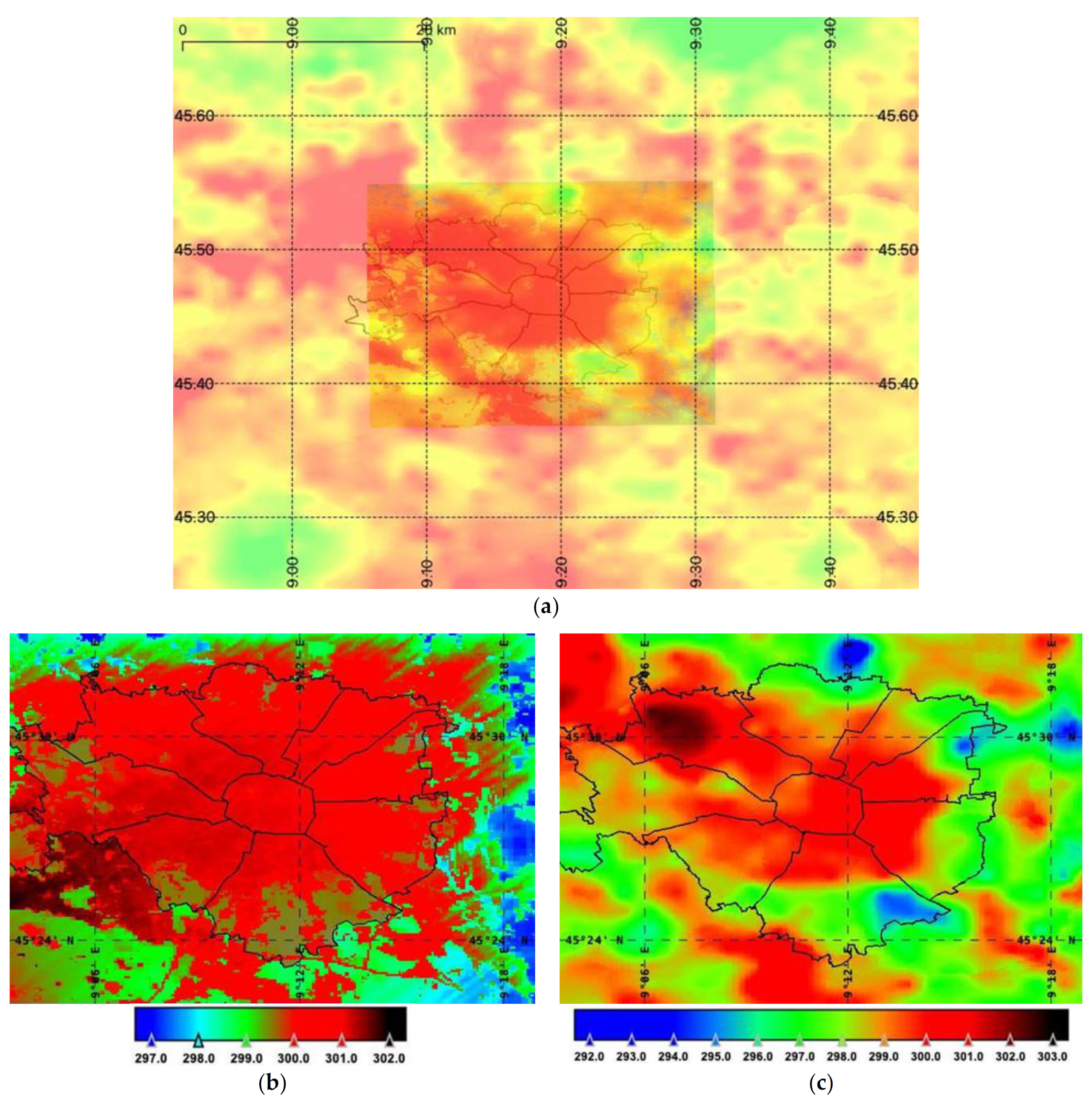
2.3.1. Comparison with ERA5/UrbClim

The last version of reanalysis by ECMWF is ERA5 [23]. A number of meteorological variables are obtained by the 4D-Var assimilation and analysis of the Integrated Forecast System (IFS) model, version CY41R2, with 137 vertical levels, a spatial resolution of 31 km, and an uncertainty estimation measured by the spread of a 10-member ensemble. On this basis, a downscaling was further developed by ECMWF for 100 European cities (Milan is among them) to obtain some ECVs at a spatial resolution of 100 m × 100 m at an hourly frequency [24]. This downscaling is the UrbClim model (UrC), which uses “a land surface scheme describing the physics of energy and water exchange between the soil and the atmosphere in the city, coupled to a 3D atmospheric boundary layer module” (cit. from UrbClim_extra_documentaion_v2.pdf (https://cds.climate.copernicus.eu/cdsapp#!/dataset/sis-urban-climate-cities?tab=doc), last accessed on 13 December 2021). The atmospheric boundary conditions are defined by meteorological input data, while the land surface data influence heat flux and evaporation. UrC data are available via the Copernicus CDS (Copernicus Climate Data Store (https://cds.climate.copernicus.eu/), last accessed on 13 December 2021) portal: Figure 4b is an example of the UrbClim product for Milan.
Unfortunately, while ERA5 has a temporal coverage since 1950 up to the present, UrC data sets cover the time interval 2008–2017, and a direct comparison with ClimaMi CoK thermal fields is only possible for the years 2016 and 2017. Moreover, while CoK fields are timely defined on a 10 min basis (being computed with 10 min mean data by AWSs nearest to the satellite pass time), UrC data are hourly: for each date, the hour selected is the nearest to the CoK field time. Therefore, the time approximation in the comparison is half an hour. Furthermore, the area covered by UrC for the city of Milan is much smaller than for ClimaMi CoK interpolations: a direct comparison is given in Figure 4a. Data were extracted from the CoK and UrC fields to combine pixel per pixel both data sets. Differences were then computed for every CoK available time: moreover, comparison is limited to winter and summer cloud free situations. As an example, in Figure 5 the differences CoK interpolation minus UrC data over Milan on 3 July 2017, 21:00 UTC, are shown in colors: negative values are up to −7 °C (in light blue) and positive up to +4 °C (in hell red). Generally, UrbClim overestimates temperatures over the city and underestimates outside, with a mean bias of −1.4 °C for this episode.
The overall Pearson correlation coefficient R, given by:
R T C ,   T U = i = 1 N ( T C ,   i T C ¯ ) T U , i T U ¯ i = 1 N T C ,   i T C ¯ 2 i = 1 N T U ,   i T U ¯ 2
where T C is the CoK interpolated temperature, T U the temperature from the UrbClim data set, and N the number of image elements (pixels), is 0.5 for the same example of Figure 5, while the covariance:
Cov T C ,   T U = i = 1 N ( T C ,   i T C ¯ ) T U , i T U ¯ N
is 0.7. Data were also extracted from UrC matrices for elements coincident with the coordinates of surface measuring stations in the Milan area covered by UrbClim. Furthermore, to provide a better and spatially related quantification of map comparison, the fuzzy Kappa statistics [25] and Moran’s index [26,27] were performed. In the first case, the similarity is based on quantity and location, and the fuzziness of location is taken by letting the fuzzy representation of a pixel be partly defined by its proximity.
The similarity of image pixels for two different temperature field values, T1 and T2, is defined by:
S T 1 , T 2 = 1 T 1 T 2 max T 1 , T 2
For the fuzziness, an exponential decay with distance appears to be appropriate considering the temperature: a radius of neighborhood of 4 and a halving distance of 2 pixels were chosen for both fields to be compared. The result statistics for overall similarity is the average similarity over the whole area.
Figure 4. A comparison example between UrbClim and CoK interpolation for the Milan area at 22:00 UTC, 3 July 2017: (a) overlapping of the UrC field over the larger CoK interpolation area; (b) the UrC air temperature at 2 m, downscaled from ERA5; (c) the CoK-interpolated near-surface air temperature. Temperature color scale in K. The UHI is clearly visible in both images almost centered over the city, but temperature range, resolution, and spatial distribution details are quite different.
Forecasting 04 00014 g004
Figure 5. Discretized air temperature difference (CoK minus UrC data) over Milan at 22:00 UTC on 3 July 2017. Bluish colors are negative values up to −7 K (light blue); red are positive differences up to +4 K (hell red). A general underestimation of the UHI by UrbClim is evident, in this case especially in the eastern and northwestern parts of Milan.
Forecasting 04 00014 g005
On the other hand, Moran’s index allows a measure of spatial (auto-) correlation based on variances and covariances. The index is defined as:
I M = N W   i = 1 N j = 1 N w ij ( T i   T ¯   )   T j   T ¯   i = 1 N T i   T ¯   2
where N is the number of samples (pixels), Ti and Tj are the variables of interest (surface temperature in our case, measured on two different maps of the same event and over the same region), wij is a matrix of spatial weights computed as an inverse distance function (with wii = 0), and W is the sum of all wij.
The expected value of Moran’s I under the null hypothesis (no spatial correlation) is given by:
E I = 1 N 1
where N is the sample number. For large samples, E(I) approaches zero: in our case, the matrices to be compared are 285 × 202 pixels and E(I) ≅ 105.
The index itself varies between −1 (total anticorrelation) and +1 (perfect autocorrelation) and can be used to compare different fields as a CrossMoran index: small differences arise depending on which is considered first: we simply take the mean value. Further, Lee’s L index [28] is a generalization for a bivariate spatial association measure, which integrates Pearson R as a spatial bivariate association measure and Moran’s I as a univariate spatial association measure using a spatial smoothing scalar. Considering the different resolution of the two types of maps, a radius of 10 was chosen as a good compromise for the spatial lag for Lee’s L, the R lagged, and the Moran statistics. A useful tool for these evaluations was presented in [29].

2.3.2. Comparison with the Weather Research and Forecasting Model

The weather research and forecasting model (WRF) is an open-source, well-known, and much-used nonhydrostatic limited area model [30]. With suitable extensions, it can also be applied for the urban environment [31]. For the city of Milan, the WRF was used for several applications [32,33] with the building environment parameterization (BEP) urban scheme [34] and at a resolution of 1 km or even less. We made use of some outputs (in default configuration: BEPd) for a direct comparison with measurements in the UCL by the 7 FOMD Network weather stations located in Milan downtown. The comparison covers two 10-day summer periods in 2014 and 2015, mainly characterized by anticyclonic weather with only occasional cloudiness and very low winds: very favorable conditions for the development of a strong nocturnal UHI effect.

3. Results

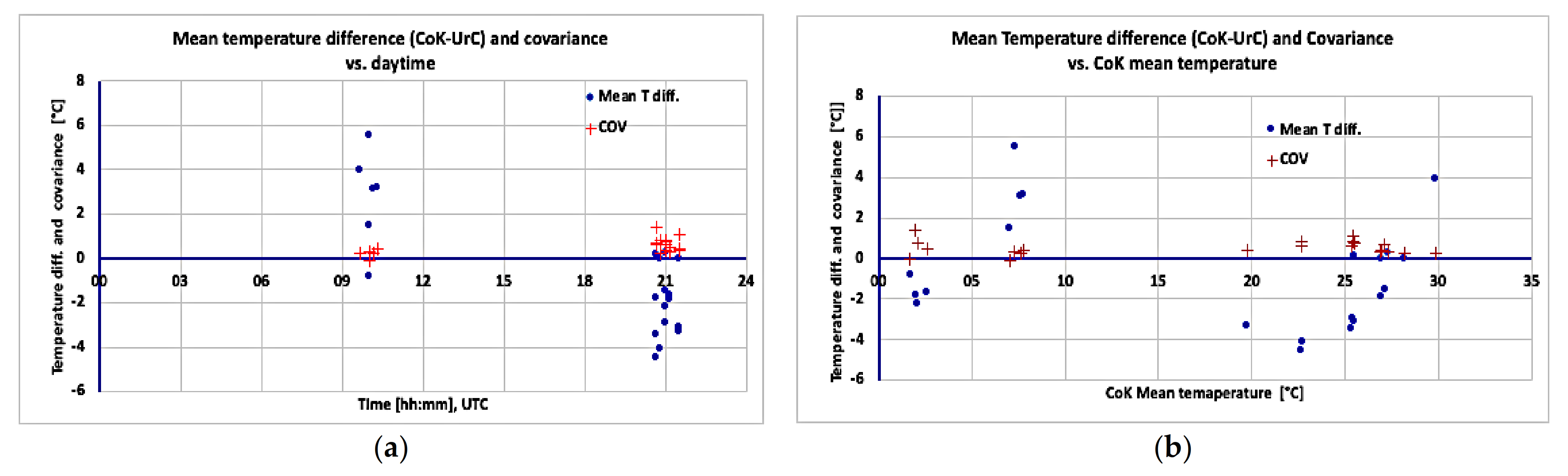
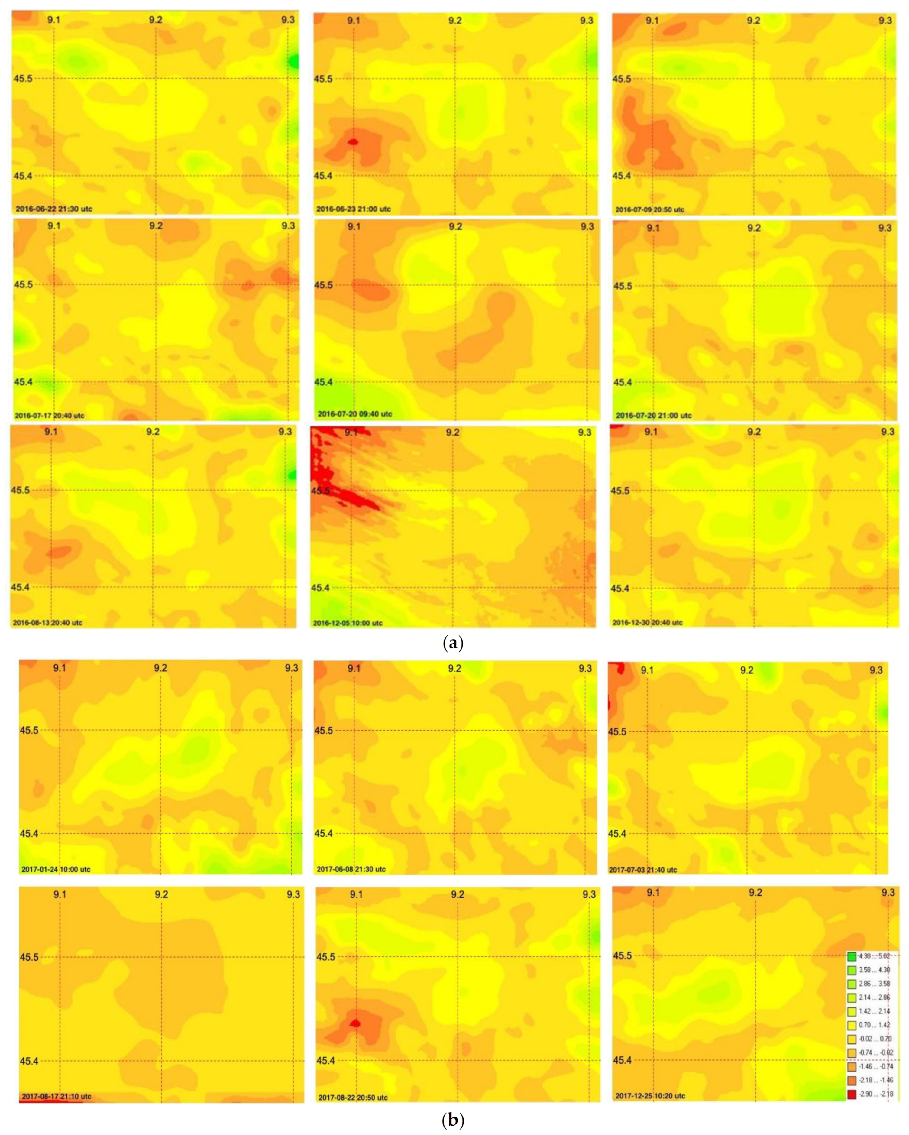
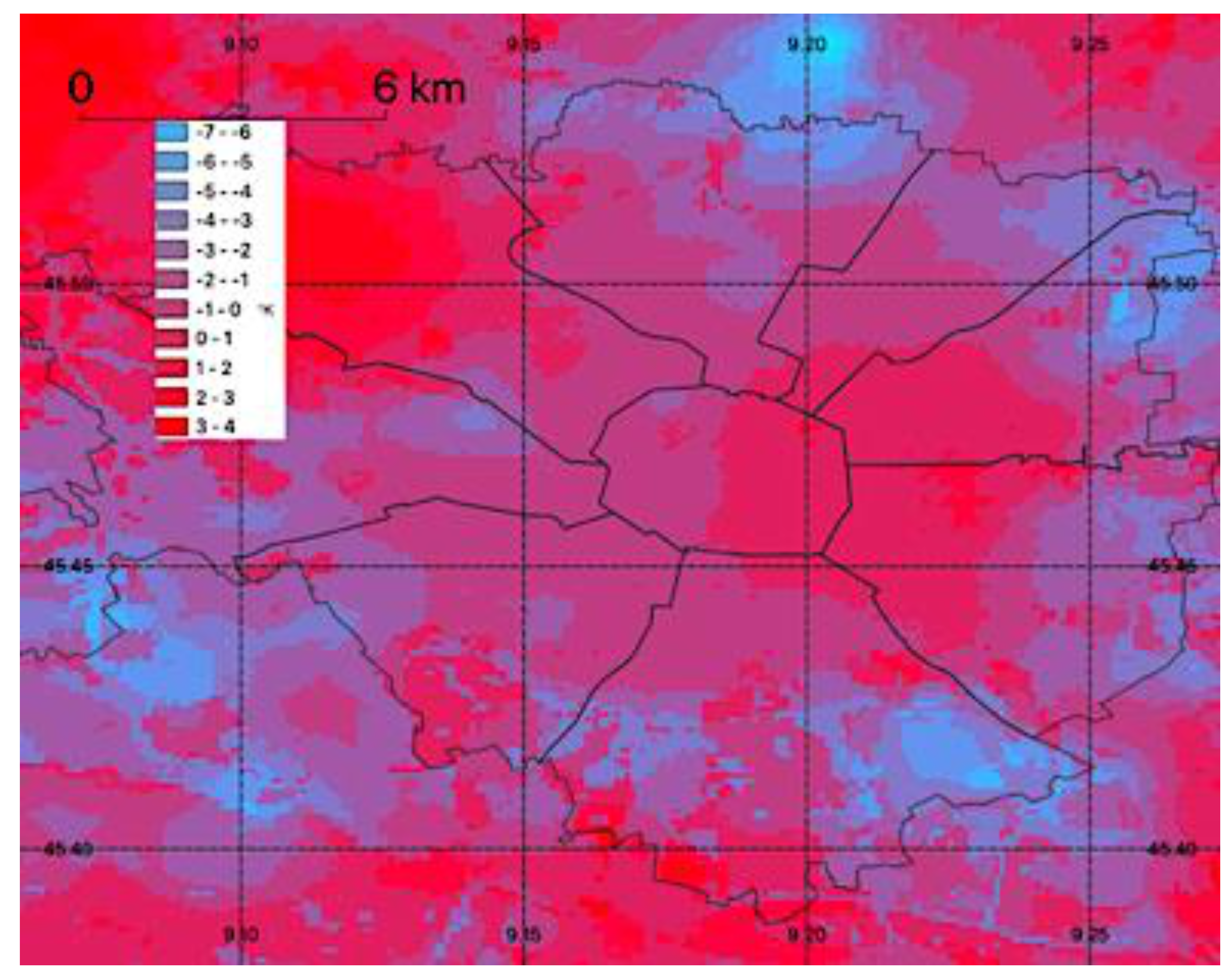
3.1. Comparison Results: ERA5/UrbClim

The comparison for each and all the available CoK episodes (21 cases, number limited by the availability of useful spaceborne data) with UrC data for Milan provides the results summarized in Table 4. The variety of meteorological and seasonal situations does not allow a straightforward conclusion, and data are not enough for situation-based statistics.
Anyway, the mean range between minimum and maximum differences is 9.3 °C, while the mean difference (“CoK minus UrC”, pixel by pixel) amounts to −2.0 ± 1.5 °C, showing a small negative bias. The mean temperature differences among CoK and UrC maps vary from −4.5 to +5.5 °C, with a clear prevalence of positive values in the morning and negative ones in the evening. The mean covariance is 0.5, ranging from almost 0 up to 1.1 regardless of daytime or season, as shown in Figure 6. The covariance is also independent of the mean temperature (representative of the season), while the mean temperature difference between CoK and UrC is smaller for lower temperatures (winter: −0.5 °C) and larger in the warmer episodes (summer: −3.0 °C).
The comparison results between measurements and UrbClim are shown in Table 5: UrC data have a mean bias “AWS minus UrC” of −2.3 ± 1.6 °C, while differences span between −11.9 °C and +6.0 °C, in substantial agreement with the result obtained for CoK data. There is anyway a large seasonal disparity, with a winter mean of only −0.5 °C and a summer mean of −3.4 °C, once again in substantial agreement with the comparison operated by using interpolated CoK data. In the winter episodes, the difference range is also smaller.
The results obtained with the fuzzy and Moran statistics for the temperature fields are summarized in Table 6, while examples of the spatial distribution of the local Lee’s L are given in Figure 7. The CoK and UrC temperature fields appear to have a relatively good spatial correlation over the city: both are catching the UHI effect. Nevertheless, there are smaller regions where correlation is weak or even negative, emphasizing the marked differences in the methods in accurately resolving the smallest-scale details.
Table 4. Comparison statistics for CoK and UrbClim (CoK–UrC) air temperature fields for all the available episodes. Pearson correlation coefficients in bold are nonsignificant at level p < 0.01.
No.Date
(d/m/y)
COK UTCDiff. Min. (°C)Diff.
Mean
(°C)
Diff. Max. (°C)Min.
Max.
Range (°C)
Pearson Corr. RCov.CoK
Mean
T
UrC
Mean
T
Mean T diff. CoK–UrCHW/Season
122/6/201621:30−9.5−3.1 ± 1.52.712.20.501.125.5 ± 1.428.6 ± 1.6−3.1Summer
223/6/201621:00−7.9−3.0 ± 1.72.910.80.320.627.1 ± 1.228.6 ± 1.6−1.5Summer
39/7/201620:50−5.6−1.5 ± 1.43.28.80.190.228.2 ± 1.128.2 ± 1.10.0Summer
417/7/201620:40−11.5−5.0 ± 1.70.512.00.310.625.3 ± 1.528.8 ± 1.3−3.4Summer
520/7/201609:400.02.5 ± 1.15.75.80.260.229.9 ± 0.925.9 ± 1.03.9HW
620/7/201621:00−5.3−1.2 ± 1.43.69.00.350.327.3 ± 1.227.1 ± 1.20.3HW
713/8/201620:40−9.9−6.0 ± 1.4−1.58.40.380.622.6 ± 1.227.1 ± 1.4−4.5Summer
85/12/201610:00−4.40.1 ± 2.04.99.3−0.05−0.17.0 ± 1.25.5 ± 1.61.5Winter
930/12/201620:40−8.0−3.2 ± 2.25.013.00.451.42.0 ± 1.23.8 ± 2.5−1.8Winter
101/1/201710:00−8.4−2.2 ± 2.53.812.2−0.02−0.11.7 ± 1.82.5 ± 1.7−0.8Winter
1124/1/201710:001.34.2 ± 1.58.97.6−0.210.37.3 ± 1.21.7 ± 1.15.5Winter
1229/1/201721:00−7.3−3.6 ± 1.0−1.06.30.600.72.1 ± 1.24.3 ± 1.0−2.2Winter
138/6/201721:30−8.4−4.8 ± 1.40.28.60.270.419.8 ± 1.123.1 ± 1.3−3.3Summer
143/7/201721:40−7.4−1.4 ± 1.33.811.20.450.725.5 ± 1.425.4 ± 1.10.1Summer
1517/8/201721:10−8.1−3.4 ± 1.22.710.80.180.326.9 ± 1.228.8 ± 1.3−1.9Summer
1622/8/201720:50−9.5−5.6 ± 1.2−1.08.50.540.822.7 ± 1.126.8 ± 1.4−4.1Summer
1728/8/201721:30−4.4−1.5 ± 1.12.97.20.450.427.0 ± 0.827.0 ± 1.20.0Summer
1829/8/201721:00−8.7−4.4 ± 1.3−0.28.50.510.825.4 ± 1.328.3 ± 1.3−2.9Summer
196/12/201710:10−4.21.7 ± 2.17.311.40.100.27.6 ± 1.74.5 ± 1.33.1Winter
2025/12/201710:20−1.91.8 ± 1.25.17.00.440.47.8 ± 1.34.6 ± 0.73.2Winter
2130/12/201721:10−6.8−3.1 ± 1.2−0.46.30.440.52.6 ± 0.94.3 ± 1.2−1.7Winter
Figure 6. Mean temperature difference between CoK and UrC maps and their covariance (a) in relation to daytime and (b) as a function of mean temperature (CoK temperature as reference). While covariances do not show any daytime and temperature dependence, temperature differences clearly tend to be positive in morning times and colder seasons and negative in the opposite cases. Most of the temperature differences are outside an estimated uncertainty interval of ±2 °C.
Forecasting 04 00014 g006
Figure 7. Spatial distribution of Lee’s L index for the comparison of CoK and UrC air temperature fields: (a) 2016 episodes and (b) 2017 episodes. The color bar in the last picture is common to all the images. Administrative borders omitted, area coincident as that in Figure 4, Milan downtown almost in the center of the pictures.
Forecasting 04 00014 g007
Table 5. Temperature differences (°C) (AWS–UrC) for the subset of 17 stations in the Milan area covered by UrbClim.
No.Date
(d/m/y)
UTCMilano Città
Studi
Milano
Bovisa
Milano CentroMilano
S. Siro
Milano
Sud
Milano
Bocconi
Milano
Bicocca
Milano
Sarpi
Cinisello
Parco
Nord
CorsicoMilano LambrateMilano
Brera
Milano
Juvara
Milano MarcheMilano ZavattariSesto
S. Giovanni Parco
Nord
Milano MaxwellMeanStd. Dev.Min.Max.
122/06/201621:30−2.3−3.2−2.4−3.2−3.2−2.8−2.6−2.7−7.2−8.3−4.7−2.5−2.4−4.1−6.9−2.2−0.4−3.62.1−8.3−0.4
223/06/201621:00−1.9−1.8−2.8−3.5−3.3−3.1−2.0−3.0−6.1−7.3−5.4−2.9−2.2−4.2−5.6−4.2−4.0−3.71.6−7.3−1.8
309/07/201620:50−0.9−0.6−0.9−2.0−1.9−1.4−0.9−0.9−4.1−5.1−4.2−0.6−0.8−1.2−2.8−1.3−3.0−1.91.4−5.1−0.6
417/07/201620:40−5.0−4.9−4.8−4.8−6.0−5.2−5.0−4.8−11.9−7.2−9.7−4.4−5.0−5.4−6.5−8.7−6.3−6.22.1−11.9−4.4
520/07/201609:40−0.11.70.94.80.10.71.10.54.33.13.01.40.41.92.42.51.91.81.4−0.14.8
620/07/201621:00−0.3−0.1−0.8−1.3−1.8−1.30.4−0.4−5.4−2.4−3.0−0.1−0.4−0.1−2.3−1.3−0.9−1.21.4−5.40.4
713/08/201620:40−5.4−5.2−5.2−6.7−6.2−5.8−5.3−5.7−9.6−9.5−9.2−4.4−5.2−6.8−8.2−7.4−7.0−6.61.6−9.6−4.4
805/12/201610:00−2.00.90.13.3−1.3−0.10.20.71.10.5−1.91.2−0.4−0.72.50.2−1.80.21.5−2.03.3
930/12/201620:40−2.5−5.8−2.9−5.4−4.7−3.9−4.6−4.1−3.1−6.1−2.3−3.5−2.4−4.8−6.6−1.9−1.8−3.91.5−6.6−1.8
1001/01/201710:00−1.10.0−1.9−1.7−4.9−3.30.6−1.40.3−0.7−2.8−2.5−0.3−2.6−0.3−0.2−0.5−1.31.5−4.90.6
1124/01/201710:002.94.13.86.02.13.13.04.76.04.05.52.32.91.44.54.74.73.91.41.46.0
1229/01/201721:00−2.3−2.5−2.1−3.1−2.3−1.7−2.6−1.7−6.5−5.6−5.6−1.9−2.0−3.0−3.4−3.5−2.9−3.11.5−6.5−1.7
1308/06/201721:30−3.7−4.0−3.8−4.1−5.0−4.2−3.3−3.8−7.8−6.6−7.3−3.7−3.8−4.5−6.3−5.8−5.7−4.91.4−7.8−3.3
1403/07/201721:40−0.1−1.1−0.3−1.5−2.3−1.1−1.4−0.9−7.3−4.0−5.2−0.3−0.2−2.3−3.6−4.1−2.3−2.22.0−7.3−0.1
1517/08/201721:10−2.2−2.1−2.4−2.6−4.6−2.9−1.6−1.9−5.8−5.9−5.4−2.4−2.1−2.9−5.2−3.3−3.3−3.31.5−5.9−1.6
1622/08/201720:50−4.4−5.3−4.6−6.3−5.9−5.3−4.7−4.6−9.5−8.0−7.9−4.4−3.9−5.3−7.9−7.2−5.9−5.91.6−9.5−3.9
1728/08/201721:30−1.5−1.4−1.7−1.7−2.3−1.7−1.5−1.3−2.1−3.4−1.5−1.3−1.2−1.4−4.1−3.2−2.1−1.90.8−4.1−1.2
1829/08/201721:00−3.5−3.7−3.3−4.0−3.7−3.5−3.6−3.2−8.3−6.7−6.7−3.3−3.4−4.5−6.3−6.3−4.6−4.61.6−8.3−3.2
1906/12/201710:100.82.22.22.00.21.42.41.42.82.62.5−0.21.6−0.52.3−5.10.91.21.9−5.12.8
2025/12/201710:203.41.62.51.11.01.91.72.12.41.53.82.43.61.22.3−5.93.71.82.2−5.93.8
2130/12/201721:10−1.5−3.4−1.3−4.2−2.4−1.7−2.2−2.4−6.6−4.1−3.7−1.9−1.3−2.6−5.2−6.2−1.1−3.01.7−6.6−1.1
Table 6. Comparison statistics of CoK and UrC air temperature fields for the available episodes.
No.DateTime (UTC)Fuzzy Num.
Average
Fuzzy Global
Matching
Moran’s I
(Map1*Map2)
Mean Cross
Moran
R LaggedLee’s L
12016/06/2221:300.990.200.960.480.60.51
22016/06/2321:000.990.190.960.320.40.33
32016/07/0920:501.000.230.970.170.20.17
42016/07/1720:400.980.160.970.280.30.29
52016/07/2009:400.990.180.990.250.30.26
62016/07/2021:001.000.330.950.330.40.36
72016/08/1320:400.980.170.960.360.40.38
92016/12/3020:400.990.210.960.430.50.45
112017/01/2410:000.980.170.970.410.50.43
132017/06/0821:300.980.170.930.270.40.31
142017/07/0321:400.980.180.940.270.30.28
162017/08/2220:501.000.260.940.340.40.37
202017/12/2510:200.990.230.990.440.50.45
Settings: Radius = 4;
exp. decay halving dist. = 2
First raster (CoK) as referenceRadius =10

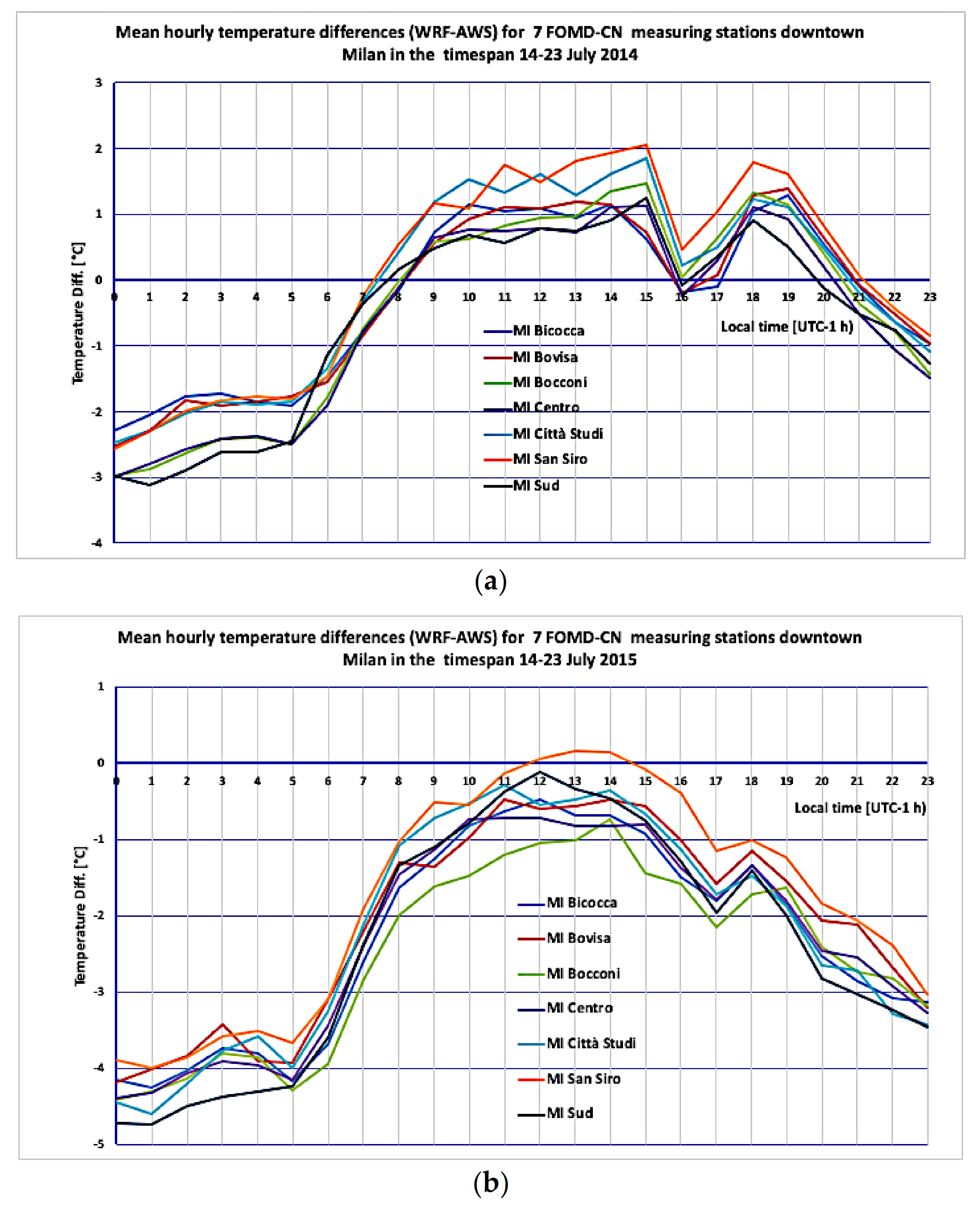
3.2. Comparison Results: WRF

The results show an average systematic underestimation of the UCL temperatures by the WRF: the mean bias (WRF computed minus FOMD Network measured) is −0.3 °C in 2014 and −2.2 °C in 2015 (Figure 8). Negative differences are systematically much larger during the night hours (−1.5 and −3.4 °C, respectively), resulting in a clear underestimation of the intensity of the typical nocturnal UHI effect over the city. The underestimation does not agree with the finding in [34]: anyway, in that case, a much smaller town is considered. During the sunlit hours, absolute values of the differences are smaller, and their sign can be even positive (−1.0 and +0.9 °C, respectively, in 2014 and 2015). As a consequence, WRF could not always account for the existence of the diurnal urban cold island, which is, however, climatologically typical in the city of Milan [18].
The differences between both years is likely related to the marked different mean temperatures in the city over the two 10-day periods: about 25 °C in 2014 with a certain range of variability among different days and 30.5 °C in 2015 characterized by an almost constant and persistent HW episode. Furthermore, the last 4 days of the 2014 period show differences that are three times as large as in the previous days. It must be noted that the mean hourly standard deviation among FOMD Network stations is always about 0.3 °C, all the seven stations being sited in a similar urban environment and their sensors exposed with the same criteria on top of typical buildings of almost equal height and with an almost constant surface albedo of 0.3. Therefore, the local climate zone classification [13] for most of them is “compact low-rise”, while only Milano Sud is “compact mid-rise”, and Bovisa and S. Siro “open high-rise”. In fact, WRF data correlate in a similar manner to all the seven FOMD Network stations in Milan downtown: correlation coefficients (R2) between WRF figures and FOMD Network data are 0.84 and 0.94, respectively: in 2015 the correlation is always significant at p < 0.01, while in 2014 the same value is found only for MI Centro; it is not significant for two stations (MI Città Studi and MI Sud), and the other ones have p < 0.1 or 0.5.
We compared the 2 m thermal fields from the WRF–BEP model with the ClimaMi CoK interpolations at a high resolution (30 m, obtained by Landsat 8 LST data): Figure 9 shows the overlapping of the two fields. From the available WRF runs, we could, unfortunately, find only three situations coincident with the CoK ones: 19 July 2014 at 10:00 UTC, 15 July 2015 at 10:00 UTC, and 22 July 2015 at 10:00 UTC. The comparison, adapting the WRF–BEP grid (84 × 66 pixels) onto the CoK-30 m grid (1001 × 1001 pixels), produced the differences shown in Figure 10: the resulting mean bias (CoK minus WRF) is −0.9 °C, essentially confirming what was previously found in this section, while the mean difference range is 4.3 °C. More evident is the general difference gradient in longitude across the area, with WRF underestimating temperature in the eastern part of the domain. On the other hand, the WRF overestimation south of the city center could be related to the fact that this region is well known to be a climatologically colder and moister area, being at a lower elevation and with a mostly agricultural land use. More interesting is the central part of the city: in this area, a small-scale variability is evident with a possible WRF overestimation, consistent with the direct comparison with measurements considering that all the three episodes are in the late morning.
We can conclude that WRF, at least in summer heat wave episodes, underestimates night temperatures of about 3 °C over the city of Milan, when the UHI effect is especially relevant, while the diurnal urban cold island could remain undetected: the results may help to improve the models in better describing the urban canopy layer, and the city of Milan could be used as a useful testbed.
Figure 8. Temperature difference between WRF simulations and FOMD Network measurements in the Milan UCL for two periods of 10 days in the month of July (a) 2014 and (b) 2015, characterized by anticyclonic weather with no precipitation, almost no cloudiness, and very low winds (favorable conditions for the development of a marked UHI) in 2015, while in 2014 there were some precipitation episodes. In 2015 mean temperatures were more than 5 °C higher than in the same period of 2014.
Forecasting 04 00014 g008
Figure 9. Overlapping of the smaller CoK field at 30 m resolution and the corresponding larger WRF field (22 July 2015 at 10:00 UTC). Both are almost centered on Milan (city center at position 45.47°N, 9.19°E). Temperature scale in K.
Forecasting 04 00014 g009
Figure 10. Temperature differences over the Milan area (CoK interpolations at 30 m resolution based on LST data from Landsat 8 minus WRF–BEP analysis): (a) at 19 July 2014, 10:00 UTC; (b) 15 July 2015, 10:00 UTC; (c) 22 July 2015, 10:00 UTC. Color scales of temperature difference are in Kelvin; administrative borders are omitted, area coincident as that in Figure 7. An E–W gradient is always evident, as well as the WRF overestimation just south of the city center (at position 45.47°N, 9.19°E), where on the contrary, there is a small-scale variability.
Forecasting 04 00014 g010

4. Discussion

The comparison results described in Section 3.1 and Section 3.2 consistently show an underestimation of the temperatures over the city of Milan by UrbClim and partly also by WRF-BEP. The mean difference is about −2 °C for UrC, with a possible seasonal variation showing smaller values in low-temperature situations in relation to warmer ones. The mean R, omitting the two unrealistic negative values, is 0.4 ± 0.1 °C, showing in general a low to moderate overall correlation. On the other hand, covariances are very variable among the considered episodes.
A similar result is found comparing UrbClim data directly with station measurements, where original information is not lost in the cokriging interpolation. The fuzzy statistics applied to compare CoK and UrC thermal fields gives a good average value, while the global matching of the maps is relatively low (0.21), showing that aside from the observed bias, the thermal fields are characterized by some differences in spatial distribution over the project area. Altogether, UrbClim appears to give a satisfactory general description of the UHI, but details even at the urban mesoscale are not well reproduced despite the declared downscaling spatial resolution at 100 m: the spatial distribution of Lee’s L shows in general better scores above the city than elsewhere, but is very variable and lacking in resolution.
On the contrary, ClimaMi CoK shows realistic details: it is able to reproduce detailed differences caused by the urban texture. Moreover, being mainly based on in situ measurements in the upper part of UCL, it can be taken as a reference. The result is confirmed by the direct match with station measurements. Some bias is also present in relation to daytime and season.
The spatial comparison with the WRF–BEP runs is based on only three episodes and cannot be considered conclusive. Anyway, a mean bias of −0.9 °C appears to be qualitatively significant. It is also consistent with the results obtained matching WRF outputs to direct measurements over the two periods of 10 summer days, where the mean bias is –1.3 ± 0.3 °C, varying from –0.1 ± 0.4 °C during daytime to –2.4 ± 0.3 °C in the night. The spatial distribution of the differences “CoK minus WRF” shows a remarkable longitudinal gradient (while it is of little or no interest in this context). Over the city area, their values are small and variable, but generally positive: this agrees with the daily variation of the differences obtained matching WRF and measurements, all the three episodes being at 10 UTC. Evidently, a more extensive comparison is required in this case, while also the model setup could be better designed (being in this case in default mode, as noted before).

5. Conclusions

An almost 10-year data set of measurements in the Milan metropolitan area UCL, mainly based on the FOMD urban meteoclimatological network and integrated with selected data from the official ARPA Lombardia monitoring network and from the amateur MeteoNetwork for a total of 61 AWSs, has been used to obtain medium- to high-resolution near-surface gridded thermal fields. In the adopted cokriging algorithm, ground air temperature by AWSs is the primary variable, while spaceborne land surface temperature by Sentinel 3 and Landsat 8 satellites is the secondary one. The results obtained, already usefully applied in resilience plans and projects by officials, engineers, and architects for the Milan metropolitan area in the framework of the ClimaMi Project, were compared with other available gridded thermal information, namely, the ERA5 downscaled reanalysis data for European cities (UrbClim) and some WRF–BEP runs over Milan made available by a research group at the University of L’Aquila.
The comparison, performed for the overlapping periods of available data from the different data sets and limited to winter and summer episodes, highlights in both cases a general agreement but also a systematic underestimation of the UHI effect over Milan. The bias can be quantified, on average, at −2 °C, while the range of this underestimation can be larger than 10 °C in the considered episodes. The spatial correlations, analyzed using fuzzy and Moran’ statistics, confirms the bias and shows a large variability in performance and location, suggesting some likely systematic trends too. Even if in this work the number of episodes is limited by data availability, specifically for spaceborne data and the WRF runs, the results imply the necessity to significantly improve modelling and downscaling methods to adequately cope with the request for punctual data posed by professionals and decision makers in order to design and effectively implement plans and projects in the current climate change situation, which in cities is a very complex subject.
We can conclude that correctly performed observations in the challenging urban environment remain of utmost importance, not only in monitoring the weather and the climate, but also specifically as an unavoidable benchmark for new modelling and downscaling products. In this case, the meteorological network extent and its affordability and operational continuity represent a major issue and require specifically dedicated resources. Integration of citizen science data, such as amateur meteorologists’ ones, has proved to be a benefit, but implies accurate data selection and validation. Furthermore, spatial analysis extends the potential of point measurements in a useful manner.
The results obtained represent a first attempt to comparatively evaluate some different techniques used to obtain high-resolution gridded thermal fields in the urban environment. Further developments shall consider a wider range of observational and modelling data sets as well as other methods of spatial analysis: further spaceborne data to improve the time and spatial resolution and more up-to-date and site-adapted meteorological models and spatial analysis methods.
Furthermore, other variables, such as humidity, wind, and precipitation, shall be considered to get a more complete description of the urban environment: analysis is already started on precipitation in the ClimaMi Project framework, while humidity and wind are the next to be analyzed: this will be a further important step towards a complete and detailed knowledge of the urban climate to address resilience to climate change.

Author Contributions

G.F. wrote the text and made the comparison statistics among AWS measurements, CoK interpolations, and UrbClim data; S.P. ensured AWS data validation and the paper revision; C.L. supervised the whole work as leader of the ClimaMi Project and revised the paper; E.M.M. performed all the CoK interpolations and the paper revision. All authors have read and agreed to the published version of the manuscript.

Funding

This research received no external funding.

Institutional Review Board Statement

Not applicable.

Informed Consent Statement

Not applicable.

Data Availability Statement

The data used in this work contributed to the climatic information of Project ClimaMi, freely available from the project portal www.progettoclimami.it (last accessed on 10 January 2022) or under request at www.fondazioneomd.it (last accessed on 10 January 2022).

Acknowledgments

Landsat LST data were downloaded from the Google Earth Engine portal; Sentinel 3 LST data were downloaded from the Copernicus portal Climate Data Store; WRF-BPM data were kindly made available by Gabriele Curci and Serena Falasca, University of L’Aquila (http://www.univaq.it/www.univaq.it, last accessed on 10 January 2022). Fondazione Cariplo partly funded Project ClimaMi. The authors thank Susanna Di Lernia (FOMD) for the final revision of the text and all the reviewers for the stimulating comments, which helped much to improve the paper.

Conflicts of Interest

The authors declare no conflict of interest.

References

  1. Santamouris, M. Recent progress on urban overheating and heat island research. Integrated assessment of the energy, environmental, vulnerability and health impact. Synergies with the global climate change. Energy Build. 2020, 207, 109482. [Google Scholar] [CrossRef]
  2. Oke, T.R.; Mills, G.; Christen, A.; Voogt, J.A. Urban Climates; Cambridge University Press: Cambridge, UK, 2017. [Google Scholar] [CrossRef] [Green Version]
  3. WMO. Guide to Instruments and Methods of Observation (CIMO Guide), 2018, WMO-No. 8. Available online: https://library.wmo.int/index.php?lvl=notice_display&id=12407#.XiGSwf5KiUk (accessed on 28 December 2021).
  4. Oke, T.R. Siting and Exposure of Meteorological Instruments at Urban Sites. In Air Pollution Modelling and Its Application XVII; Springer: Berlin/Heidelberg, Germany, 2007; pp. 615–632. [Google Scholar] [CrossRef]
  5. Mills, G.; Cleugh, H.; Emmanuel, R.; Endlicher, W.; Erell, E.; McGranahan, G.; Ng, E.; Nickson, A.; Rosenthal, J.; Steemer, K. Climate Information for Improved Planning and Management of Mega Cities (Needs Perspective). Procedia Environ. Sci. 2010, 1, 228–246. [Google Scholar] [CrossRef] [Green Version]
  6. Muller, C.L.; Chapman, L.; Grimmond, C.S.B.; Young, D.T.; Cai X-M. Sensors and the city: A review of urban meteorological networks. Int. J. Climatol. 2013, 33, 1585–1600. [Google Scholar] [CrossRef]
  7. Hulley, G.C.; Ghent, D.; Göttsche, F.M.; Guillevic, P.C.; Mildrexler, D.J.; Coll, C. Land Surface Temperature. In Taking the Temperature of the Earth; Elsevier: Amsterdam, The Netherlands, 2019; pp. 57–127. [Google Scholar] [CrossRef]
  8. Toparlar, Y.; Blocken, B.; Maiheu, B.; van Heijst, G.J.F. A review on the CFD analysis of urban microclimate. Renew. Sustain. Energy Rev. 2017, 80, 1613–1640. [Google Scholar] [CrossRef]
  9. Jänicke, B.; Miloševic, D.; Manavvi, S. Review of User-Friendly Models to Improve the Urban Micro-Climate. Atmosphere 2021, 12, 1291. [Google Scholar] [CrossRef]
  10. Vuckovic, M.; Hammerberg, K.; Mahdavi, A. Urban weather modeling applications: A Vienna case study. Build. Simul. 2020, 13, 99–111. [Google Scholar] [CrossRef] [Green Version]
  11. Wackernagel, H. Cokriging. In Multivariate Geostatistics; Springer: Berlin/Heidelberg, Germany, 1995. [Google Scholar] [CrossRef]
  12. Montoli, E.; Frustaci, G.; Lavecchia, C.; Pilati, S. High-resolution climatic characterization of air temperature in the urban canopy layer. Bull. Atmos. Sci. Technol. 2021, 2, 7. [Google Scholar] [CrossRef]
  13. Stewart, I.D.; Oke, T.R. Local climate zones for urban temperature studies. Bull. Am. Meteorol. Soc. 2012, 93, 1879–1900. [Google Scholar] [CrossRef]
  14. Chapman, L.; Muller, C.L.; Young, D.T.; Warren, E.L.; Grimmond, C.S.B.; Cai, X.; Ferranti, E.J.S. The Birmingham Urban Climate Laboratory: An Open Meteorological Test Bed and Challenges of the Smart City. Bull. Am. Meteorol. Soc. 2015, 96, 1545–1560. Available online: https://journals.ametsoc.org/view/journals/bams/96/9/bams-d-13-00193.1.xml (accessed on 23 November 2021). [CrossRef]
  15. Cheval, S.; Micu, D.; Dumitrescu, A.; Irimescu, A.; Frighenciu, M.; Iojă, C.; Tudose, N.C.; Davidescu, Ș.; Antonescu, B. Meteorological and Ancillary Data Resources for Climate Research in Urban Areas. Climate 2020, 8, 37. [Google Scholar] [CrossRef] [Green Version]
  16. Borghi, S.; Favaron, M.; Frustaci, G. Climate network: A climatological network for energy applications in urban areas. IEEE Instrum. Meas. Mag. 2014, 17, 18–23. [Google Scholar] [CrossRef]
  17. Curci, S.; Lavecchia, C.; Pilati, S.; Paganelli, C. High quality sustainable monitoring in cities for climatological services. WMO-IOM Report-No 132. In Proceedings of the 2018 WMO/CIMO Technical Conference on Meteorological and Environmental Instruments and Methods of Observation (CIMO-TECO) “Towards Fit-for-Purpose Environmental Measurements”, Amsterdam, The Netherlands, 8–11 October 2018; Available online: https://library.wmo.int/index.php?lvl=notice_display&id=20734#.XAejlq5KuUl (accessed on 15 November 2021).
  18. Curci, S.; Lavecchia, C.; Frustaci, G.; Paolini, R.; Pilati, S.; Paganelli, C. Assessing measurement uncertainty in meteorology in urban environments. Meas. Sci. Technol. 2017, 28, 104002. [Google Scholar] [CrossRef] [Green Version]
  19. Frustaci, G.; Pilati, S.; Lavecchia, C. Canopy Urban Heat Island observations in Milano: Methodological aspects and recent climatology. In Proceedings of the European Geosciences Union General Assembly, Vienna, Austria, 7–12 April 2019; Volume 2019, p. 6052. Available online: https://meetingorganizer.copernicus.org/EGU2019/orals/31288 (accessed on 22 April 2021).
  20. Frustaci, G.; Pilati, S.; Lavecchia, C. Climatology of the Milano Canopy Urban Heat Island by means of an operational urban meteorological network. In Proceedings of the AISAM 2° National Congress, Napoli, Italy, 24–26 September 2019; Available online: https://www.fondazioneomd.it/pubblicazioni (accessed on 22 April 2021).
  21. Goovaerts, P. Geostatistics in soil science: State-of-the-art and perspectives. Geoderma 1999, 89, 1–45. [Google Scholar] [CrossRef]
  22. Kilibarda, M.; Hengl, T.; Heuvelink, G.B.M.; Gräler, B.; Pebesma, E.; Tadić, M.T.; Bajat, B. Spatio-temporal interpolation of daily temperatures for global land areas at 1 km resolution. J. Geophys. Res. Atmos. 2014, 119, 2294–2313. [Google Scholar] [CrossRef] [Green Version]
  23. Hersbach, H.; Bell, B.; Berrisford, P.; Hirahara, S.; Horanyi, A.; Muñoz-Sabater, J.; Nicolas, J.; Peubey, C.; Radu, R.; Schepers, D.; et al. The ERA5 global reanalysis. Q. J. R. Meteorol. Soc. 2020, 146, 1999–2049. [Google Scholar] [CrossRef]
  24. De Ridder, K.; Lauwaet, D.; Maiheu, B. UrbClim—A fast urban boundary layer climate model. Urban Clim. 2015, 12, 21–48. [Google Scholar] [CrossRef] [Green Version]
  25. Hagen-Zanker, A. Fuzzy set approach to assessing similarity of categorical maps. Int. J. Geogr. Inf. Sci. 2003, 17, 235–249. [Google Scholar] [CrossRef] [Green Version]
  26. Moran, P.A.P. Notes on Continuous Stochastic Phenomena. Biometrika 1950, 37, 17–23. [Google Scholar] [CrossRef]
  27. Chen, Y.G. An analytical process of spatial autocorrelation functions based on Moran’s index. PLoS ONE 2021, 16, e0249589. [Google Scholar] [CrossRef]
  28. Lee, S.-I. Developing a Bivariate Spatial Association Measure: An Integration of Pearson’s r and Moran’s I. J. Geogr. Syst. 2001, 3, 369–385. [Google Scholar] [CrossRef]
  29. Visser, H.; de Nijs, T. The Map Comparison Kit. Environ. Modeling Softw. 2006, 21, 346–358. [Google Scholar] [CrossRef]
  30. Skamarock, W.C.; Klemp, J.B.; Dudhia, J.; Gill, D.O.; Liu, Z.; Berner, J.; Wang, W.; Powers, J.G.; Duda, M.G.; Barker, D.M.; et al. A Description of the Advanced Research WRF Version 4; NCAR Technical Note NCAR/TN-556+STR; UCAR: Boulder, CO, USA, 2019; p. 145. [Google Scholar] [CrossRef]
  31. Barlage, M.; Miao, S.; Chen, F. Impact of physics parameterizations on high-resolution weather prediction over complex urban areas. J. Geophys. Res. 2016, 121, 4487–4498. [Google Scholar] [CrossRef] [Green Version]
  32. Falasca, S.; Ciancio, V.; Salata, F.; Golasi, I.; Rosso, F.; Curci, G. High albedo materials to counteract heat waves in cities: An assessment of meteorology, buildings energy needs and pedestrian thermal comfort. Build. Environ. 2019, 163, 106242. [Google Scholar] [CrossRef]
  33. Falasca, S.; Curci, G.; Salata, F. On the association between high outdoor thermo-hygrometric comfort index and severe ground-level ozone: A first investigation. Environ. Res. 2021, 195, 110306. [Google Scholar] [CrossRef]
  34. Gohil, K.; Jin, M.S. Validation and Improvement of the WRF Building Environment Parametrization (BEP) Urban Scheme. Climate 2019, 7, 109. [Google Scholar] [CrossRef] [Green Version]
Table 1. Automatic weather stations (AWS) of the 3 different networks in and around Milan: FOMD (Fondazione Osservatorio Meteorologico Milano Duomo), ARPA (Regional Environmental Protection Agency of Lombardy), MeteoNetwork (MN): citizen–scientists’ meteorological association.
No.NameLongitude E
WGS84 (°)
Latitude N
WGS84 (°)
Altitude
m.s.l. (m)
Owner/ManagerAWS
1Milano Città Studi9.22965245.479995171FOMDVaisala WXT520
2Milano Bovisa9.16383745.502578150FOMDVaisala WXT520
3Milano Centro9.19490945.459641135FOMDVaisala WXT520
4Milano San Siro9.12537745.478607198FOMDVaisala WXT520
5Milano Sud9.20049745.431289129FOMDVaisala WXT520
6Milano Bocconi9.18771145.450826147FOMDVaisala WXT520
7Milano Bicocca9.21158245.510169143FOMDVaisala WXT520
8Milano Sarpi9.17595145.479822141FOMDVaisala WXT520
9Gaggiano9.03388345.406186129FOMDVaisala WXT520
10Magenta8.88397245.466300159FOMDVaisala WXT520
11Rho9.03952145.529664184FOMDVaisala WXT520
12Cinisello Balsamo9.21159145.555619167FOMDVaisala WXT520
13Seregno9.19841545.652056241FOMDVaisala WXT520
14Vimercate9.36851745.613961208FOMDVaisala WXT520
15Melzo9.42361445.504597140FOMDVaisala WXT520
16San Donato Milan.9.25797745.424985122FOMDVaisala WXT520
17Lacchiarella9.13740845.321406115FOMDVaisala WXT520
18Legnano8.91879545.595506226FOMDVaisala WXT520
19Saronno9.04939745.636727228FOMDVaisala WXT520
20Lodi9.48875745.30756292FOMDVaisala WXT520
21Vigevano8.85929945.318034117FOMDVaisala WXT520
22Osio Sotto9.61173745.620556182ARPA /
23Rivolta d’Adda9.52068945.444091102ARPA /
24Osnago9.38855645.677698234ARPA /
25Cavenago d’Adda9.56266045.26927467ARPA /
26Sant’Angelo Lodig.9.37966045.26066760ARPA./
27Misinto9.06639045.661382247ARPA /
28Castello d’Agogna8.70057245.246801106ARPA /
29Cornale8.91414545.04007774ARPA /
30Pavia Folperti9.16463845.19467677ARPA /
31Pavia SS 359.14666445.18062271ARPA /
32Voghera9.01749444.99027395ARPA /
33Busto Arsizio R.8.82387845.626387242ARPA /
34Somma Lombardo8.71269145.649537210ARPA /
35Arconate8.84732245.548517182ARPA /
36Cinisello Parco N.9.20560345.542665142ARPA /
37Corsico9.09741145.436109119ARPA /
38Lacchiarella9.13451745.32451897ARPA /
39Motta Visconti8.98856345.281956100ARPA /
40Rodano9.35349745.472580112ARPA /
41S.Colombano L.9.48624945.186999140ARPA /
42Milano Brera9.18911045.471656122ARPA /
43Milano Juvara9.22231545.473226122ARPA /
44Milano Lambrate9.25751545.496780120ARPA /
45Milano Marche9.19093445.496316129ARPA /
46Milano Zavattari9.14178645.476063122ARPA /
47Landriano9.26715345.32059488ARPA /
48Seregno Ovest9.17903445.653843224MNDavis Vantage Pro+2
49Giussano9.20547045.690773265MNDavis Vantage Pro 2
50Sesto S. Giovanni PN9.20962245.538144141MNDavis Vantage Pro 2
51Lodi San Bernardo9.52012545.29913278MNDavis Vantage Pro+2
52Monza V. Sgambati9.26147545.596264180MNDavis Vantage Pro 2
53Mezzana Bigli8.85000045.07000076MNDavis Vantage Pro 2
54Treviglio9.57516945.510036125MN Davis VantagePro +2
55Lodi Viale Europa9.49406345.30551380MNDavis Vantage Pro 2
56Saronno9.02498345.634373220MNDavis Vantage Pro 2
57Lesmo via Po9.30796545.655836241MNDavis Vantage Pro 2
58Milano Maxwell9.24053245.498166138MNDavis Vantage Pro 2
59Carpiano Centro9.27087345.338421105MNDavis Vantage Pro 2
60Monza Parco9.28602245.619501180MNDavis Vantage Pro 2
61Trecate S. Maria8.73000045.420000136MNDavis Vantage Pro 2
Publisher’s Note: MDPI stays neutral with regard to jurisdictional claims in published maps and institutional affiliations.

