ARIMA Time Series Models for Full Truckload Transportation Prices


Eli Broad College of Business, Michigan State University, East Lansing, MI 48824, USA
Forecasting 2019, 1(1), 121-134; https://doi.org/10.3390/forecast1010009
Submission received: 14 September 2018
/
Revised: 21 September 2018
/
Accepted: 24 September 2018
/
Published: 26 September 2018
Abstract
:The trucking sector in the United States is a $700 billion plus a year industry and represents a large percentage of many firms’ logistics spend. Consequently, there is interest in accurately forecasting prices for truck transportation. This manuscript utilizes the autoregressive integrated moving average (ARIMA) methodology to develop forecasts for three time series of monthly archival trucking prices obtained from two public sources—the Bureau of Labor Statistics (BLS) and Truckstop.com. BLS data cover January 2005 through August 2018; Truckstop.com data cover January 2015 through August 2018. Different ARIMA models closely approximate the observed data, with coefficients of variation of the root mean-square deviations being 0.007, 0.040, and 0.048. Furthermore, the estimated parameters map well onto dynamics known to operate in the industry, especially for data collected by the BLS. Theoretical and practical implications of these findings are discussed.
1. Introduction
The trucking industry in the United States is estimated to be approximately $700 billion annually, transports nearly 71 percent of freight, and employs and estimated 2 million individuals who operate heavy duty trucks [1,2]. Given an estimated 90 percent plus of this freight moves under contract rates that typically last for a year [3], both shippers and trucking companies (termed carriers) have a strong incentive to accurately forecast trucking prices (termed rates). The ability to develop accurate pricing forecasts is challenging due to uncertainty inherent in the price of oil—which is subject to substantial swings due to geopolitical forces and technological changes (e.g., hydraulic fracturing in the United States)—coupled with trucking services being a derived demand that fluctuates based on changes to macro-economic conditions and the seasonality of industrial production and retail sales. Further issues arise because the supply curve for trucking capacity is relatively inelastic in the near term (e.g., 3 to 6 months) due to the lead time for buying new equipment and training truck drivers [4,5]. Thus, when demand for trucking services rapidly increases, prices tend to increase, as has occurred in late 2017 and throughout 2018, until more capacity comes online [6].
Given these various forces, the question that naturally arises is can accurate forecasts be generated for macro-level trucking prices? To date, limited research has been conducted concerning trucking pricing, and the research that has been conducted does not investigate industry-level prices. One set of studies explores pricing of the less-than-truckload (LTL) freight—shipments less than 10,000 pounds. Baker [7] examines LTL carriers’ pricing practices using survey data from 24 large LTL carriers concerning pricing approaches for 64 city-pairs to examine (i) the variance in the base rates carriers charge for shipments between the same two cities, (ii) the extent carriers offer discounts from these base rates, and (iii) carriers’ class rate practices—specifically, the extent they employ “pure scales”. Smith, Campbell, and Mundy [8] use data from a large LTL carrier to estimate a regression model predicting revenue at the customer-lane unit of analysis using characteristics of the transported freight (e.g., total shipments, total weight of shipments, etc.). Kay and Warsing [9] utilize nonlinear regression to develop a model that estimates rates using publicly available data for LTL base rates; their study also develops nonlinear regression models for full truckload prices, likewise using public data. Özkaya et al. [10] built a regression model to predict LTL prices using shipment, shipper, and carrier characteristics from data for approximately 485 thousand shipments over a 3-month horizon from 43 shippers and 128 carriers.
A second set of studies has examined factors that affect the price of shipments on the full truckload spot market—a market where one-time exchanges take place between shippers and carriers [11]. Lindsey et al. [12] estimate regression models to predict lane-level and shipment-level prices that a third party logistics provider paid for spot market transactions. Their models incorporated shipment (e.g., miles, number of stops, etc.), lane (e.g., ratio of shipments outbound from a region relative to inbound), and market (e.g., nationwide rates) predictors. Budak, Ustundag, and Guloglu [13] utilize quantile regression and artificial neural network models to forecast spot market prices for both full truckload and LTL shipments in Turkey for a third party logistics firm. Scott [11] examines how shipment and carrier factors affect the price premium for spot market shipments relative to contract rate shipments using several years of transaction data from one shipper. Joo, Min, and Smith [14] benchmark prices paid by two shippers for full truckload services by estimating a regression model where prices are a function of distance to explore whether price differences across shippers stem from carriers charging different fixed versus variable costs.
This paper differs from the above works in a few ways. First, unlike the above studies that forecasted prices at detailed levels, this manuscript focuses on developing models to predict macro-level trucking prices including (i) the price carriers providing long-distance full truckload general freight transport receive for their services [3], (ii) national spot market rates for general freight full truckload transport, and (iii) national spot market rates for refrigerated full truckload transport. Devising models to predict national truckload prices is valuable for strategic decision-making at shippers and carriers. Shippers can use these models to better budget for transportation costs and inform their contract negotiations. For example, if shippers observe that spot market rates are expected to rise, they may want to move quickly to lock-in contract rates before spot rates rise, as rising spot rates drive up contract rates [15]. Carriers can utilize these models to inform equipment purchases, plan expansions, and allocate equipment to different markets. Regarding the latter point, since spot market rates tend to be substantially higher than contract rates [11], if carriers observe that spot rates are likely to rise, carriers may wish to allocate a greater share of their capacity to the spot market to increase revenue [16]. A second contribution is shifting emphasis away from forecasting prices using shipment, customer, carrier, and lane characteristics towards focusing on how prices evolve based on the underlying temporal dynamics of the freight market as captured by the autoregressive integrated moving average (ARIMA) modeling framework. The ARIMA framework [17] provides a useful means for examining the evolution of freight rates given how the parameters of such models align with dynamic forces [18] known to affect freight rates.
The remainder of this paper is structured in four sections. Section 2 describes the ARIMA methodology and explains the meaning of estimated parameters in the context of motor carrier rates. Section 2 also discusses data sources. Section 3 contains the results. Section 4 describes implications and highlights limitations. Section 5 offers a brief conclusion and suggests future research directions.
2. Materials and Methods
2.1. ARIMA Methodology and Trucking Pricing
The ARIMA methodology provides a useful framework for understanding the evolution of motor carrier rates because (i) the method has a substantial degree of flexibility and (ii) the theoretical meaning of ARIMA parameters map well to dynamic forces expected to affect trucking prices. Given freight rates have risen over time due to wage growth and rising fuel costs, this presentation will assume a first difference specification at a monthly level (the standard frequency industry-wide rates are reported) to ensure the price time series is weakly stationary (e.g., constant mean, constant variance, and the correlation between rates at any two occasions in the series will decline towards zero as the occasions become further temporally separated) [19]. Thus, ΔRatet = Ratet − Ratet−1 where t represents months. Consider first an ARIMA(0,1,1) model for rates as shown in Equation (1):
In Equation (1), parameter captures the expected month-over-month change in freight rates while captures the effects of idiosyncratic shocks—Browne and Nesselroade [18] refer to as a “random shock” variable—in the current month that increase or decrease rates beyond the expected change. A positive value for indicates that a random shock that resulted in an increase (decrease) in freight rates in the prior month will carry over to the current month by increasing (decreasing) freight rates beyond the expected month-over-month change [18]. An example of this is hurricane relief efforts [20], such as those undertaken for Hurricanes Katrina in 2005 and Harvey in 2017. Hurricane Harvey relief efforts resulted in a substantial increase in the demand for freight services in September 2017 [21]. Thus, we would expect the increase in freight rates for September 2017 (time t − 1) relative to August 2017 (time t − 2) to be substantially more than usual (i.e., would be positive). The model in Equation (1) suggests that this idiosyncratic shock to September rates relative to August rates will positively affect the change in rates from October (time t) relative to September. Critically, a property of the one-month moving average is that the effect of the prior unexpected shock affects prices for only the next month [18]; thus, moving average effects quickly dissipate. Returning to the hurricane relief example, the one-month positive moving average implies that the spike in September rates will only affect October’s rates; this effect will have completely dissipated by November. Moreover, given that moving-average models typically assume that the random shocks are independent over time, such models are most appropriate in contexts where the dynamic force bringing about change in the focal variable (ΔRate in this example) is assumed to have limited continuity across time [18].
Consider now an ARIMA(1,1,0) model shown in Equation (2):
Equation (2) differs from Equation (1) in that the change in trucking rates in the current month relative to the prior month is a function of the change in rates from the prior month relative to two months ago. The key theoretical difference between these models is that the model in Equation (2) suggests that changes in freight rates are driven by prior changes in freight rates in a persistent manner [18], with the degree of persistence captured by . Consequently, an autoregressive specification is theoretically consistent with settings where dynamic forces bringing about change are expected to have some degree of persistence. For example, the model in Equation (2) is theoretically aligned with the idea that changes in supply and demand conditions that shaped prior changes in freight rates will continue to operate by affecting subsequent prices for some time. Consequently, one would expect to have a positive sign in this context, indicating freight rates in the current month increase (decrease) when freight rates rose (fell) in the prior month. This aligns with [18] (p. 421) description that “the AR model seems a potentially valuable representation for psychological trait where the expectation is “repeatable” behavior from occasion to occasion unless something happens to disrupt it.” Moreover, the autoregressive specification allows for idiosyncratic price shocks in the prior months to have persistent effects on subsequent months’ price changes. This is apparent when recognizing:
Consequently, Equation (2) can be rewritten as shown in Equation (4):
Equation (4) illustrates that idiosyncratic shocks from the prior period propagate based on and decay in an exponential manner such that a random shock at time t contributes to future observations at time t + n as [18] (p. 421). This illustrates how the moving-average versus autoregressive specifications imply theoretically distinct processes for the dynamic forces bringing about change in the focal variable.
The natural extension is to couple the moving-average and autoregressive effects in the same model. Combining Equations (1) and (2) yields the ARIMA(1,1,1) model in Equation (5):
The ARIMA(1,1,1) model implies that changes in freight rates are a function of both changes in prior rates and prior idiosyncratic shocks. In particular, if both and are positive, the model indicates that the effects of idiosyncratic shocks in the prior time period decay more rapidly than the exponential decay assumed by the pure autoregressive model. Such a model seems highly plausible given the industry dynamics that bring about freight rates. However, as no prior studies exist for estimating such models, model development will take an empirical approach informed through an iterative evaluation of data characteristics (e.g., autocorrelation and partial autocorrelation plots) and model diagnostics (e.g., whether residuals follow a white noise sequence).
2.2. Data Sources
Data for this study were obtained from two public sources. The first source is the Bureau of Labor Statistics (BLS) producer price index (PPI) for full truckload, long-distance, general freight trucking services [22]. These data are part of the BLS’s long-running PPI program and measure the prices truckload motor carriers receive for general freight transportation of long-distance shipments. These data are reported at a monthly level in index format with December 2003 representing a value of 100. This study utilizes data starting in January 2005 through August 2018. These data are not seasonally adjusted and incorporate information regarding base rates, fuel surcharges, and discounts. PPI data have been utilized by economists studying the evolution of prices [23,24]; thus, there is reason to view these data as having a strong degree of validity. This series is called Truckload.BLS.
The second and third series were obtained from Truckstop.com [25], one of the largest online load boards where shippers can post freight for spot market transportation. These data concern the average monthly price shippers paid for transportation of freight using dry vans—the primary type of equipment used to haul general freight—and refrigerated trailers. Every month Truckstop.com publishes such data, and this information is picked up and disseminated by industry news websites. These specific data were collected through archived searches of Commercial Carrier Journal’s website. An example of one of these monthly postings can be found at [26]. Using this approach, monthly data were assembled from January 2015 through August 2018. These data are reported in dollars per mile, are not seasonally adjusted, and include fuel surcharges. Given the coverage of freight on Truckstop.com, it is reasonable to view these data as having an acceptable degree of validity in capturing national spot market full truckload prices in the respective sectors. These series are denoted as DryVan.Truckstop and Refrig.Truckstop. These data are available online at File S1.
3. Results
3.1. Descriptive Statistics and Data Transformations
To give the reader a sense of how these data behave, Figure 1 plots Truckload.BLS from January 2005 through August 2018. Figure 1 shows that truckload prices have trended upward over time, though two periods of downturn exist. The first, and most severe, downturn occurred in the latter half of 2008 through early 2009 during the height of the Great Recession. This took place because of the dramatic decline in freight demand coupled with the pronounced decrease in fuel costs. The second decline took place in late 2014 through 2016. This period bucked the upward trend because fuel costs declined and demand for truckload transportation decreased due to an excessive level of inventories [27] and weak industrial output [28]. The dramatic rise in late 2017 through 2018 is consistent with industry observation that strong demand coupled with tight capacity have resulted in substantial price increases [6]. Figure 2 plots DryVan.Truckstop and Refrig.Truckstop; these data show a similar pattern of decreasing rates through 2015 and 2016 and a strong upward movement in late 2017 that continued relatively unabated through July 2018. Figure 3 overlays Truckload.BLS and DryVan.Truckstop for the same period; these data correlate r = 0.92. Lastly, Figure 4 plots the month-over-month percentage change in Truckload.BLS and DryVan.Truckstop. Figure 4 illustrates that spot market prices are far more volatile than the BLS’s broader index. This occurs because, as previously noted, the vast majority of freight hauled by trucks is priced according to contract rates that are negotiated for a year or longer [3]. Furthermore, because contract rates are negotiated for longer time horizons, prices swing less dramatically in response to demand shocks (e.g., increases or decreases in the volume of freight needing transport) than spot market rates. In contrast, as explained by [29], substantial swings in spot prices are possible because these prices are highly sensitive to changes in supply and demand conditions.
Figure 1 and Figure 2 suggest the three series are not stationary due to their upward trend. To evaluate stationarity, Elliott, Rothenberg, and Stock (ERS) efficient unit root tests [30] were conducted using the AUTOREG procedure in SAS Version 13.1, letting the routine determine the optimum lag length. For all three series, the ERS tests failed to reject the null hypothesis that the data were I(1) non-stationary. Consequently, all series were first-differenced at a monthly level (e.g., February 2018 less January 2018). To evaluate whether the first-differenced data were stationary, ERS tests were conducted on the differenced data. These ERS tests strongly reject the null hypothesis that the data are I(1) non-stationary in favor of the alternative hypothesis that the differenced data are I(0) stationary. Consequently, the first-differenced data are utilized for all analyses.
3.2. Results
All ARIMA models were estimated using the ARIMA procedure in SAS Version 13.1 using full information maximum likelihood. As noted earlier, identification of the specific form for the ARIMA model was based on empirical considerations. Beginning with Truckload.BLS, a well-performing ARIMA model that resulted in a white noise residual series with approximately normally distributed residuals was an ARIMA(1,1,0) model with estimates as follows (note, t-statistics reported below estimates in parentheses):
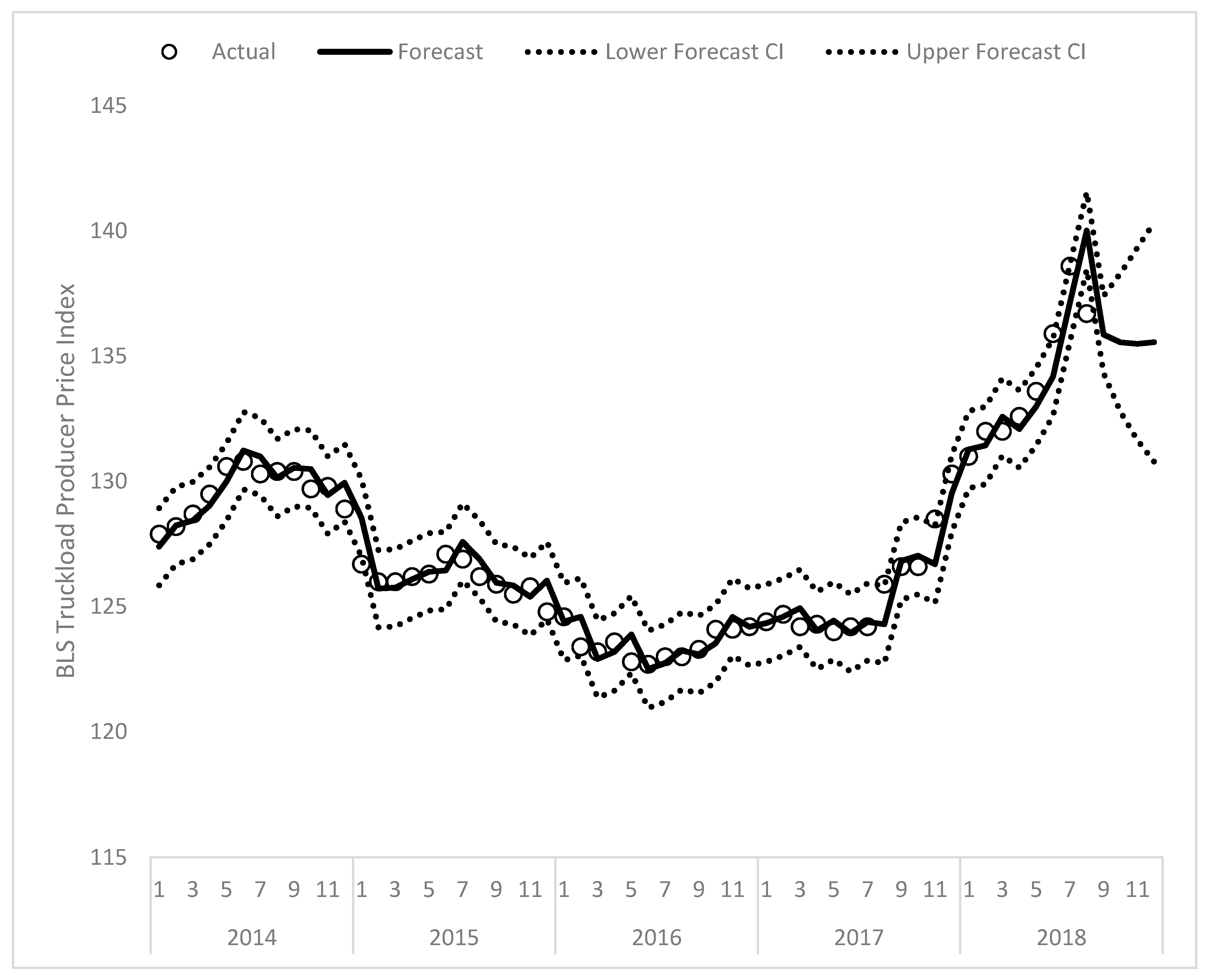
The forecasted results from fitting this model are plotted in Figure 5 from January 2014 through December 2018 (i.e., with a 4-month lead). Inspecting Figure 5, the model appears to perform well for forecasting purposes for the most recent data. Likewise, Figure 6 plots the forecasted values for February 2005 through December 2010; the model similarly performs well with these data. This performance is achieved despite the substantial swings that take place in Truckload.BLS. Overall forecast accuracy was examined by calculating the coefficient of variation of the root mean-square deviation (CV.RMSD). Letting represent the forecasted value, . the observed value, and the average observed value, CV.RVSD is calculated as where T is the total number of observations in the fitted series. CV.RMSD is 0.007 for the entire series, indicating the expected deviation is roughly 0.7 percent of the mean. Regarding interpretation of the parameters, the autoregressive estimate of 0.489 suggests a substantial degree of persistence in that changes in the current month go on to meaningfully affect prices for the next three months. Interestingly [31], note that the rate adjustment process takes approximately four to six months, which is very consistent with the reported estimates. Concerning future predictions, the model forecasts that prices will remain relatively steady through the rest of 2018, which is consistent with industry expectations given the most recent pricing data from August suggests rates may have peaked in July [29]. Specifically, Truckload.BLS exhibited a 1.37 percent decrease in August 2018 relative to July 2018, which is the largest one-month change since January 2015 relative to December 2014.
Turning now to DryVan.Truckstop, the ARIMA model found to perform well features a first difference and a single autoregressive parameter at a six period lag. Thus, this model can be notated as an ARIMA(0,1,0)(1,0,0)6 model with the following structure:
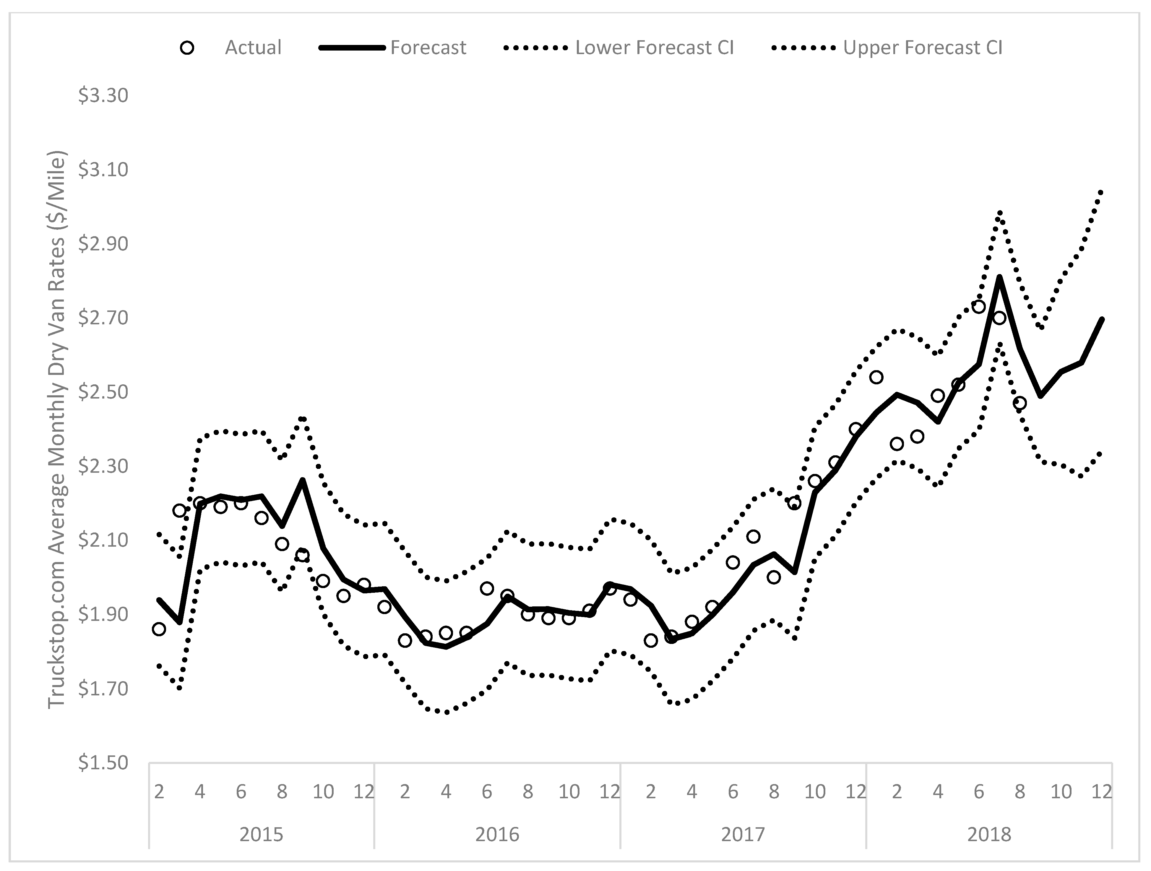
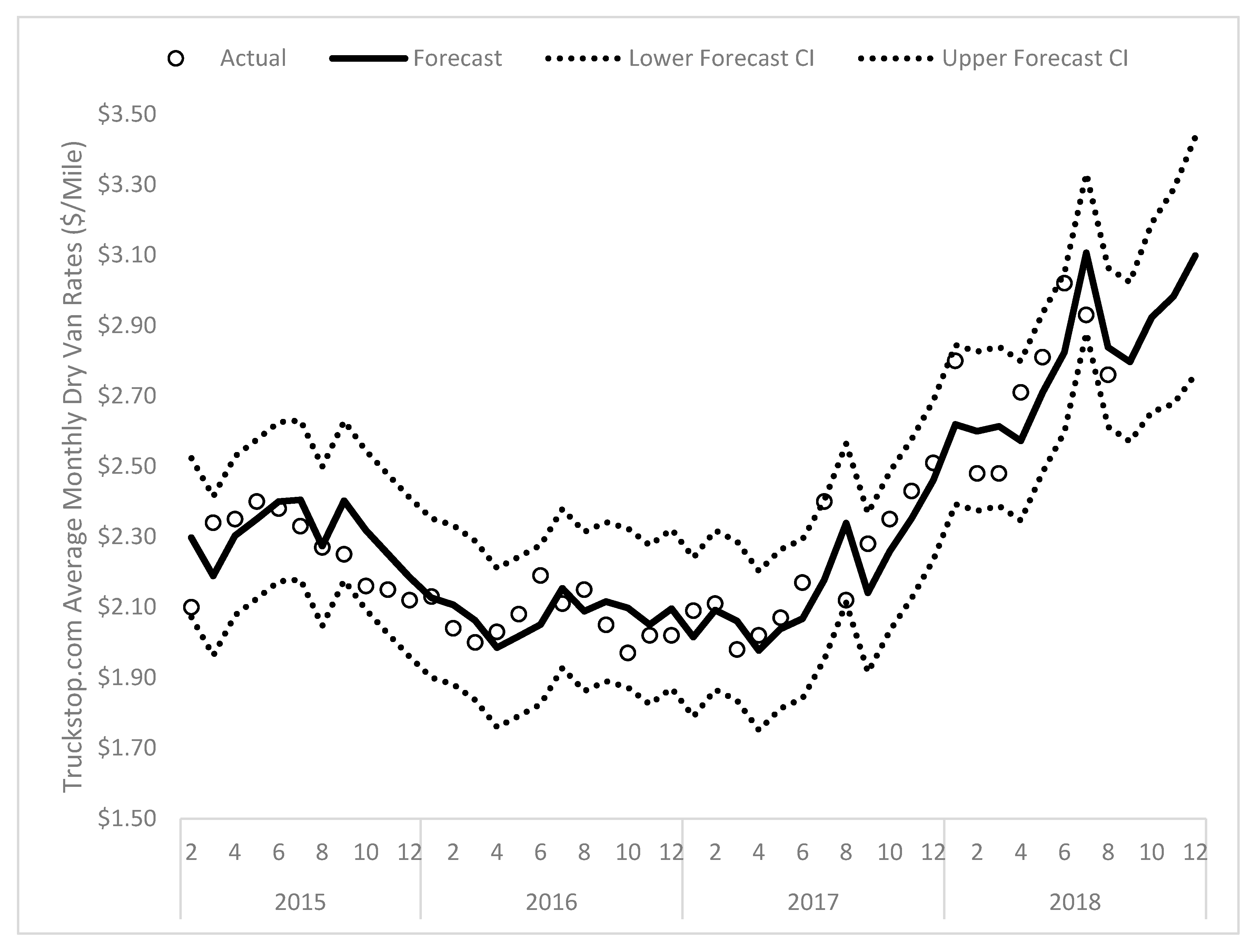
The forecast from this model is plotted in Figure 7. While the six month lag structure is somewhat difficult to explain (this will be expanded upon in the next section), the model does perform well for forecasting purposes, with the CV.RMSD being 0.042. Thus, the expected deviation of the forecasted values is approximately 4.2 percent of the dollars per mile reported by Truckstop.com. Figure 7 indicates that the model expects spot market rates to increase from the recent August dip, which is consistent with the spike in spot market transportation that occurs in the autumn to stock stores for holiday sales and transport e-commerce shipments. As such, while the model’s structure was not expected, it appears to capture dynamics that have occurred over the past three-and-a-half years.
The final series to consider is Refrig.Truckstop. The ARIMA model found to perform well features a first difference, a single autoregressive parameter at a six-month lag, and a single moving-average parameter with a one-month lag. Thus, this model can be notated as an ARIMA(0,1,1)(1,0,0)6 model with the following structure:
The forecast from this model is plotted in Figure 8. As before, while the six month lag structure is somewhat difficult to explain, the moving-average parameter has a clear theoretical interpretation in that random shocks in the prior month subsequently impact current month prices before quickly dissipating. This is consistent with arguments that spot market pricing is, to some extent, determined by random shocks [29]. Overall, this model performs well for forecasting, with the CV.RMSD being 0.049, which indicates the expected deviation of the forecasted values is approximately 4.9 percent of the reported value for Refrig.Truckstop.
4. Discussion
The central aim in this manuscript has been to develop simple yet accurate time series forecasts for different time series capturing the price of freight movements using trucks in the United States and, in doing so, shed some light on the underling dynamic forces that give rise to changes in these prices. In this regard, these analyses highlight both similarities and differences in the dynamic forces that shape trucking prices in the United States.
Consider first Truckload.BLS. The finding that an autoregressive process with one-month lag results in good model fit indicates a high degree of persistence in price changes. As noted by [18], the autoregressive specification is consistent with dynamic forces that show some degree of stability. This finding aligns with the fact these pricing data should display a substantial degree of persistence given the vast majority of freight in the full truckload general freight sector is priced according to contract rates [3,32], and newly formed contract rates tend to adjust to changes in underlying supply and demand conditions over several (e.g., four) months [31]. Furthermore, these data suggest that changes in the prices shippers pay for transportation of full truckload general freight shipments tend to show a modest change, even when the industry experiences a substantial time period where conditions strongly favor carriers [29]. For example, even in the height of the current freight market in 2018, the largest month-over-month percent change in Truckload.BLS was 1.99 percent (July 2018 relative to June 2018), and the largest year-over-year percent change was 11.59% (July 2018 relative to July 2017). While such price changes are certainly large, they are nowhere near the magnitude of changes in spot market rates, which saw an 8.33 percent month-over-month rise in June 2018 relative to May 2018 and a 33.82 percent year-over-year rise in June 2018 relative to June 2017. Thus, the central implication from this analysis is that shippers and carriers can accurately forecast prices measured by the BLS for general freight, full truckload transportation and should expect these data to evolve following an ARIMA(1,1,0) process. Consequently, it seems reasonable for shippers and carriers to utilize the model developed in this manuscript, in addition to other forecasts, to develop their forward projections of where industry conditions will be in the near future.
Turning now to the spot market rates from Truckstop.com, while adequate forecasts were developed for these data, a more cautionary tone is necessary due to (i) these data exhibiting several substantial month-over-month swings, as can be seen in Figure 4, and (ii) the fact that spot market prices are heavily driven by failure of carriers to secure capacity from their contract carriers [29]. A common terminology utilized in the industry is that high spot market rates indicate “failing routing guides” [29], where the routing guide refers to the set of carriers for which shippers have contract rates on a given lane (i.e., origin-destination pair) [3,33]. A shipper’s routing guide fails when its contract carriers refuse to haul shipments for various reasons such as (i) inadequate fuel surcharges such that carriers make little profit on the haul, (ii) contract rates being below what carriers could make hauling other loads, (iii) carriers not having equipment available at the time and location the shipper requires, (iv) carriers fearing they cannot obtain another shipment outbound from the destination of the current shipment, (v) higher than expected demand on the lane, and (vi) high variability in demand on a lane [16]. Given the reason for these refusals is often triggered by unforecastable events, such as carriers preferring to haul rescue relief shipments following major natural disasters, spot rates are more likely to show substantial fluctuation. A good example of this can be seen by comparing the spot market and BLS data from December 2017 through February 2018. Figure 2 and Figure 4 show the spot market exhibited radical swings in this period, with DryVan.Truckstop increasing 5.83 percent from December to January and then falling 7.09 percent in February from January. In contrast, Truckload.BLS increased 0.54 percent in January from December and 0.76 percent in February from January. Regarding the estimated parameters, while the one-month positive moving average effect for the Refrig.Truckstop series makes theoretical sense in that it suggests unexpected price increases (decreases) in the prior month increase (decrease) prices in the following month [18], there is less explanation for why the six-month lag autoregressive coefficient plays such a strong predictive role. One potential explanation is that this coefficient is capturing the fact that the freight market is quite seasonal, with February and August tending to represent quieter periods, which can be seen in Figure 4’s price declines. Likewise, June and December, traditionally strong months for spot market shipments due to firms pushing out orders prior to the 4th of July and holiday sales, are likewise separated by six months. Consequently, more caution is urged when forecasting spot market prices data vis-à-vis the BLS data.
As with all research, this work has limitations that should be considered when evaluating and generalizing the findings. One limitation stems from the nature of the underlying pricing data in that it is possible some of the month-over-month variation stems from the composition of shipments having different characteristics (e.g., origin-destination locations, average length of haul, etc.). For example, if the composition of spot market shipments differs on a month-over-month basis (e.g., one month features a greater proportion of desirable shipments), average price per mile will show some variation due to this composition itself, regardless of changes in supply and demand. Likewise, the BLS index is formed by surveying a large number of carriers each month; to the extent these carriers haul freight with different characteristics, one would expect that slight differences in the index values may arise due to the shipment composition. While admittedly a limitation, to the extent that changing shipment composition is affecting prices, it should obscure time series effects associated with changing supply and demand conditions. In other words, we can think of this as creating measurement error [18] that should inhibit the performance of ARIMA models fit to observed time series.
A second limitation is the limited length of the time series for the Truckstop.com data. While ideally these data could have been obtained further back, repeated internet searches failed to yield results. In a similar vein, these findings are confined to North American truckload freight operations, and in the case of the BLS data, truckload motor carriers headquartered in the United States. Thus, generalizing these findings to other countries or to other industry sectors (e.g., the flatbed sector), should be avoided.
Another concern, and one often expressed by industry practitioners seeking to utilize statistical models for applied uses, is whether the reported models are “true” in the sense utilized in everyday language. Often to the chagrin of the asker, the answer—as in the case here—is assuredly “no”; the models reported herein are not true in the literal sense. However, this fact is tempered because, as [34] (p. 2) wrote, “Models, of course, are never true, but fortunately it is only necessary that they be useful. For this, it is usually needful only that they not be grossly wrong.” Likewise, [35] (p. 512) state, “Models usually are formalizations of processes that are extremely complex … The best that one can hope for is that some aspect of a model may be useful for description, prediction, or synthesis.” Given the high predictive accuracy of the reported models, their ability to adequately respond to several substantial changes in prices, and the fact their estimated parameters map to dynamics known to operate in the industry, especially for the BLS data, suggests the ARIMA models estimated here meet these criteria.
5. Conclusions
Truck transportation represents a substantial portion of a firm’s spending on logistics activities [7,11]; consequently, developing accurate forward-looking projections is essential for budgeting and negotiating purposes. Motor carriers further need accurate forecasts to plan equipment purchases and inform their negotiation strategies [36]. The models developed in this manuscript provide a useful tool in this regard, as their high predictive accuracy suggests stakeholders can use their outputs as one input into their strategic planning routines.
This manuscript points to many directions for further study. One extension is to develop similar forecasting models for other transportation cost series tracked by the BLS, especially for rail transportation, to evaluate whether such series display a similar pattern of temporal effects. A second direction for further research is to explore the extent that changes in index composition may indeed contribute to a measurement error in index values. This would be more readily doable using data from private parties, as data from BLS is subject to confidentiality restrictions. Another avenue is to explore how contract and spot market rates are temporally related. There are strong arguments from industry experts that spot market and contract rates are cointegrated [19] in that a long-run equilibrium exists given that a large spread between spot and contract rates results in contract rates adjusting upward, whereas a narrow spread results in contract rates adjusting downward [29,37]. Examining how this equilibrium comes about would be highly valuable. Similarly, given strong industry arguments that spot market rates drive contract rates [29,31,37], exploring the nature of this relationship (e.g., its magnitude, the lag length, etc.) would have strong practical applications.
Supplementary Materials
The following are available online at https://www.mdpi.com/2571-9394/1/1/9/s1, File S1: data file.
Funding
This research received no external funding.
Acknowledgments
The author would like to thank Alex Scott and William Muir for their numerous valuable comments throughout this project. The assistance of Francetta Willett, who works for the BLS and oversees this data used in this manuscript, is greatly appreciated for clarifying the different rate aspects captured by BLS. The usual disclaimer about errors applies.
Conflicts of Interest
The author declares no conflict of interest.
References
- American Trucking Association. Reports, Trends & Statistics. 2018. Available online: https://www.trucking.org/News_and_Information_Reports_Industry_Data.aspx (accessed on 9 September 2018).
- Viscelli, S. Driverless? Autonomous Trucks and the Future of the American Trucker. Center for Labor Research and Education, University of California, Berkeley, and Working Partnerships USA. 2018. Available online: http://www.wpusa.org/files/reports/driverless.pdf (accessed on 10 September 2018).
- Caplice, C. Electronic markets for truckload transportation. Prod. Oper. Manag. 2007, 16, 423–436. [Google Scholar] [CrossRef]
- Miller, J.W.; Schwieterman, M.A.; Bolumole, Y.A. Effects of motor carriers’ growth or contraction on safety: A multiyear panel analysis. J. Bus. Logist. 2018, 39, 138–156. [Google Scholar] [CrossRef]
- Phillips, E.E. Get in Line: Backlog for Big Rigs Stretches to 2019. Available online: https://www.wsj.com/articles/get-in-line-backlog-for-big-rigs-stretches-to-2019-1534500005 (accessed on 10 September 2018).
- Phillips, E.E.; Smith, J. As Shipping Costs Soar, Supply Chains Get a Makeover. Available online: https://www.wsj.com/articles/as-shipping-costs-soar-supply-chains-get-a-makeover-1529244003 (accessed on 10 September 2018).
- Baker, J.A. Emergent pricing structures in LTL transportation. J. Bus. Logist. 1991, 12, 191–202. [Google Scholar]
- Smith, L.D.; Campbell, J.F.; Mundy, R. Modeling net rates for expedited freight services. Transp. Res. E Logist. Transp. Rev. 2007, 43, 192–207. [Google Scholar] [CrossRef]
- Kay, M.G.; Warsing, D.P. Estimating LTL rates using publicly available empirical data. Int. J. Logist.-Res Appl. 2009, 12, 165–193. [Google Scholar] [CrossRef]
- Özkaya, E.; Keskinocak, P.; Joseph, V.R.; Weight, R. Estimating and benchmarking less-than-truckload market rates. Transp. Res. E Logist. Transp. Rev. 2010, 46, 667–682. [Google Scholar] [CrossRef]
- Scott, A. The value of information sharing for truckload shippers. Transp. Res. E Logist. Transp. Rev. 2015, 81, 203–214. [Google Scholar] [CrossRef]
- Lindsey, C.; Frei, A.; Alibabai, H.; Mahmassani, H.S.; Park, Y.W.; Klabjan, D.; Reed, M.; Langheim, G.; Keating, T. Modeling Carrier Truckload Freight Rates in Spot Markets. Working Paper. 2013. Available online: http://docs.trb.org/prp/13-4109.pdf (accessed on 10 September 2018).
- Budak, A.; Ustundag, A.; Guloglu, B. A forecasting approach for truckload spot market pricing. Transp. Res. A Pol. 2017, 97, 55–68. [Google Scholar] [CrossRef]
- Joo, S.J.; Min, H.; Smith, C. Benchmarking freight rates and procuring cost-attractive transportation services. Int. J. Logist. Manag. 2017, 28, 94–205. [Google Scholar] [CrossRef]
- Smith, J. Trucking’s Tight Capacity Squeezes U.S. Businesses. Available online: https://www.wsj.com/articles/truckings-tight-capacity-squeezes-u-s-businesses-1533816002 (accessed on 10 September 2018).
- Scott, A.; Parker, C.; Craighead, C.W. Service refusal in supply chains: Drivers and deterrents of freight rejection. Transp. Sci. 2017, 54, 1086–1101. [Google Scholar] [CrossRef]
- Box, G.E.P.; Jenkins, G.M. Time Series Analysis: Forecasting and Control; Holden-Day: San Francisco, CA, USA, 1970. [Google Scholar]
- Browne, M.W.; Nesselroade, J.R. Representing psychological processes with dynamic factor models. In Psychometrics: A festschrift to Roderick P. McDonald; Maydeu-Olivares, A., McArdle, J.J., Eds.; Lawrence Erlbaum Associates Publishers: Mahwah, NJ, USA, 2005; pp. 415–452. [Google Scholar]
- Enders, W. Applied Econometric Time Series, 4th ed.; John Wiley & Sons: Hoboken, NJ, USA, 2015. [Google Scholar]
- Tsai, M.T.; Regan, A.; Saphores, J.D. Freight transportation derivatives contracts: State of the art and future developments. Transp. J. 2009, 48, 7–19. [Google Scholar]
- FTR. Hurricane Harvey Disrupting Freight Transportation in Gulf Region—Nearly Ten Percent of U.S. Trucking Impacted. Available online: https://ftrintel.com/news/hurricane-harvey-disrupting-freight-transportation-in-gulf-region-nearly-ten-percent-of-us-trucking-impacted (accessed on 10 September 2018).
- Federal Reserve Bank of St. Louis. Producer Price Index by Industry: General Freight Trucking, Long-Distance Truckload. Available online: https://fred.stlouisfed.org/series/PCU484121484121 (accessed on 9 September 2018).
- Gwin, C.R. Asymmetric price adjustment: Cross-industry evidence. South Econ. J. 2009, 76, 249–265. [Google Scholar] [CrossRef]
- Peltzman, S. Prices rise faster than they fall. J. Political Econ. 2000, 108, 466–502. [Google Scholar] [CrossRef]
- Truckstop.com. Available online: https://truckstop.com/ (accessed on 10 September 2018).
- CCJ Staff. Indicators: Spot Market Rates soften Some after Historic Run. Available online: https://www.ccjdigital.com/indicators-spot-market-rates-soften-some-after-historic-summer-run/ (accessed on 7 September 2018).
- Duel, D.; Christopher, C.G. Steady as She Goes. Supply Chain Quarterly. 2017, pp. 33–36. Available online: http://www.supplychainquarterly.com/topics/Inventory/20170825-steady-as-she-goes/ (accessed on 10 September 2018).
- Mitchell, J.U.S. Manufacturing Activity Loses Momentum. Available online: https://www.wsj.com/articles/u-s-manufacturing-activity-loses-momentum-1533138906 (accessed on 10 September 2018).
- Harding, M. The Epic Battle of the Bull and Bear—The Double-Edged Sword of Rapid Truckload Rate Increases. Available online: https://www.chainalytics.com/the-epic-battle-of-bull-and-bear-the-double-edged-sword-of-rapid-truckload-rate-increases/ (accessed on 10 September 2018).
- Elliott, G.; Rothenberg, T.J.; Stock, J.H. Efficient tests for an autoregressive unit root. Econometrica 1996, 64, 813–836. [Google Scholar] [CrossRef]
- Commercial Carrier Journal. Contract Rates Dart Upward to Catch Soaring Spot Market Rates. 2018. Available online: https://www.ccjdigital.com/contract-rates-dart-upward-to-catch-soaring-spot-market-rates/ (accessed on 10 September 2018).
- Sheffi, Y. Combinatorial auctions in the procurement of transportation services. Interfaces 2004, 34, 245–252. [Google Scholar] [CrossRef]
- Caplice, C.; Sheffi, Y. Optimization-based procurement for transportation services. J. Bus. Logist. 2003, 24, 109–128. [Google Scholar] [CrossRef]
- Box, G.E.P. Some problems of statistics and everyday life. J. Am. Stat. Assoc. 1979, 74, 1–4. [Google Scholar] [CrossRef]
- Cudeck, R.; Henly, S.J. Model selection in covariance structures analysis and the “problem” of sample size: A clarification. Psychol. Bull. 1991, 109, 512–519. [Google Scholar] [CrossRef] [PubMed]
- Bowman, R.J. Advice for Shippers Facing Rising Freight Rates in 2017. Available online: https://www.supplychainbrain.com/blogs/1-think-tank/post/24752-advice-for-shippers-facing-rising-freight-rates-in-2017 (accessed on 10 September 2018).
- Harding, M. Drinking from the Transportation Market Fire Hose—Part 2. Available online: https://www.chainalytics.com/drinking-transportation-market-fire-hose-part-2/ (accessed on 10 September 2018).
Figure 1.
Plot of Truckload.BLS at a monthly level from January 2005 through August 2018.
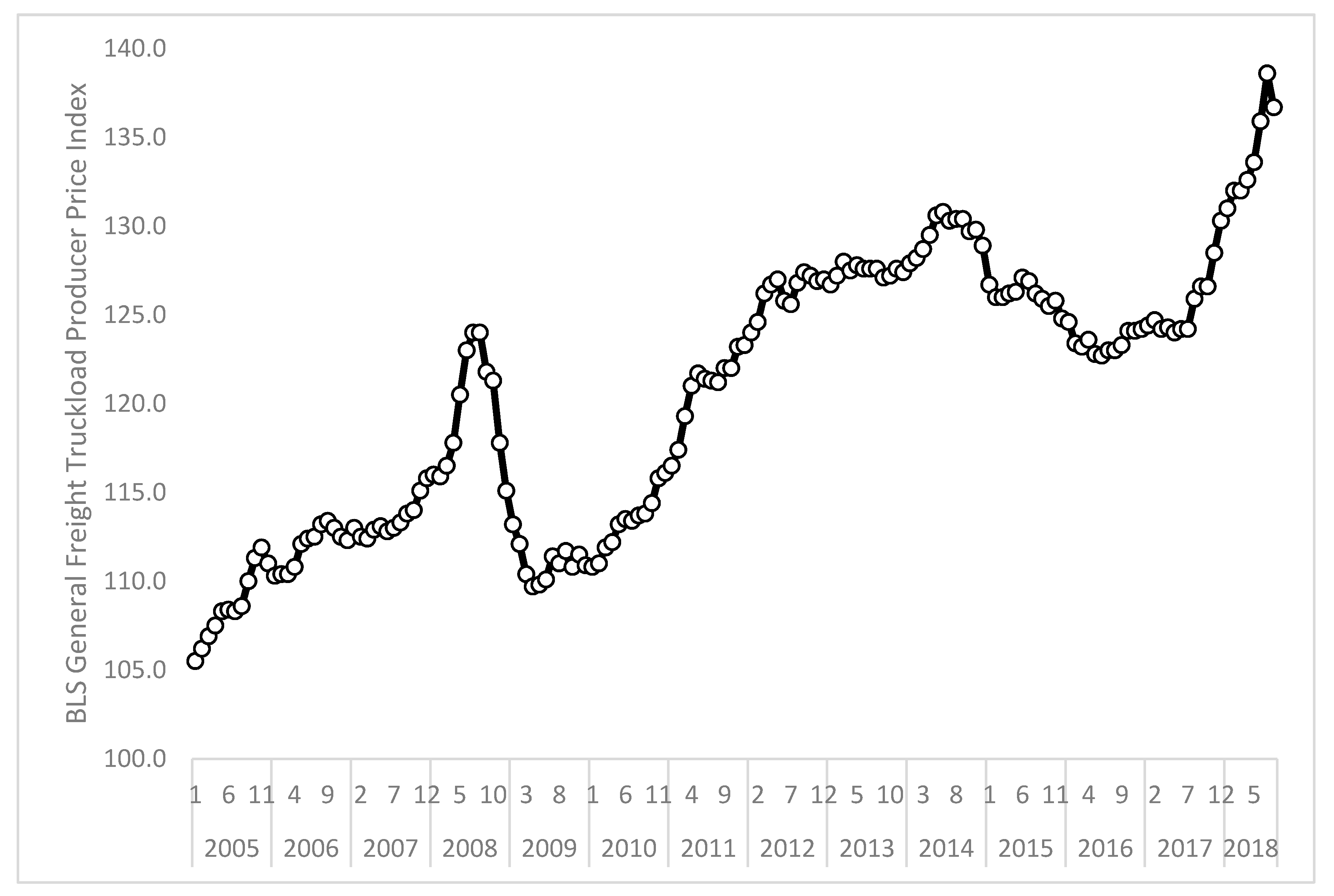
Figure 2.
Plot of DryVan.Truckstop and Refrig.Truckstop for January 2015 through August 2018.
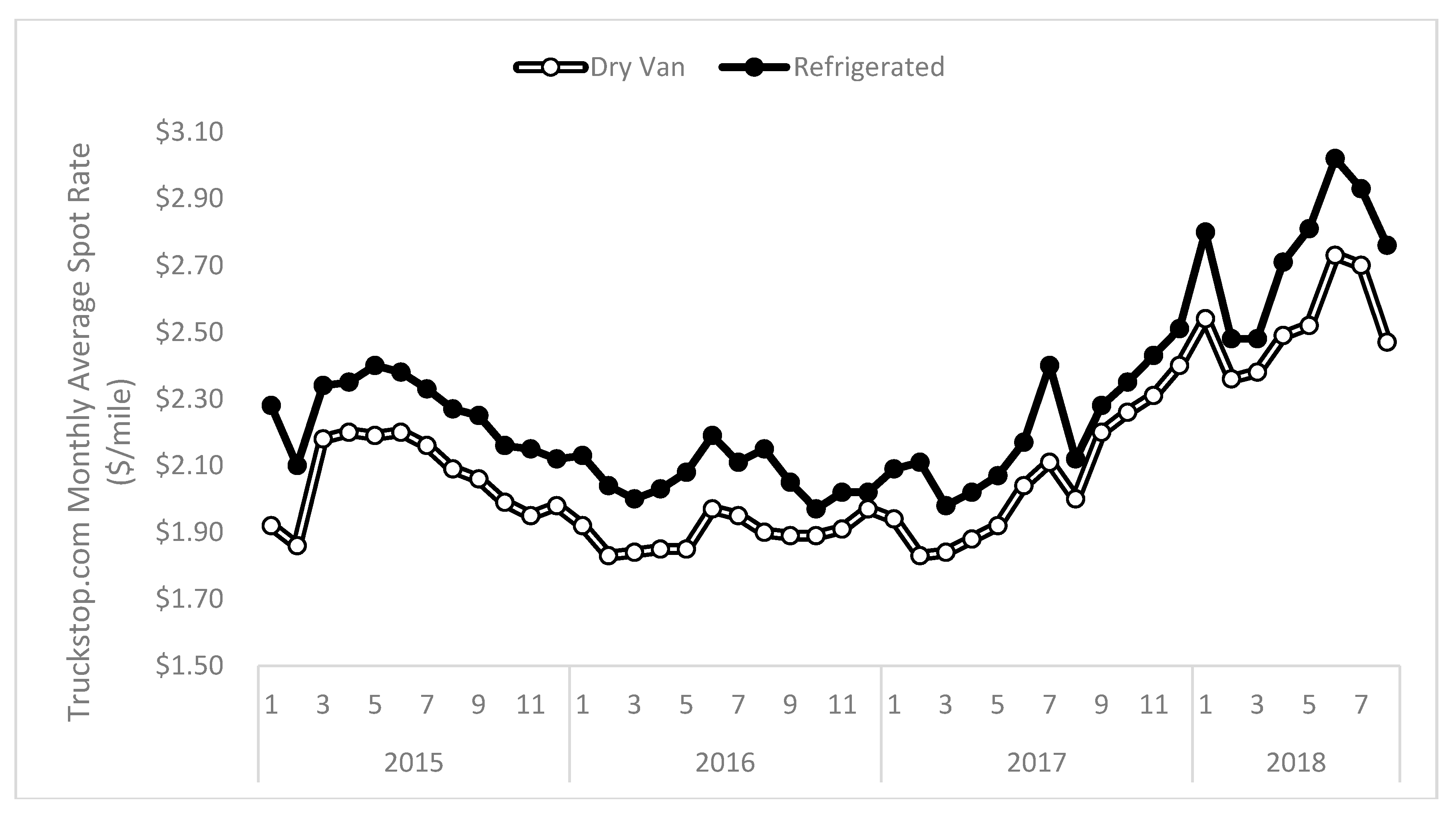
Figure 3.
Plot of Truckload.BLS and DryVan.Truckstop for January 2015 through August 2018.
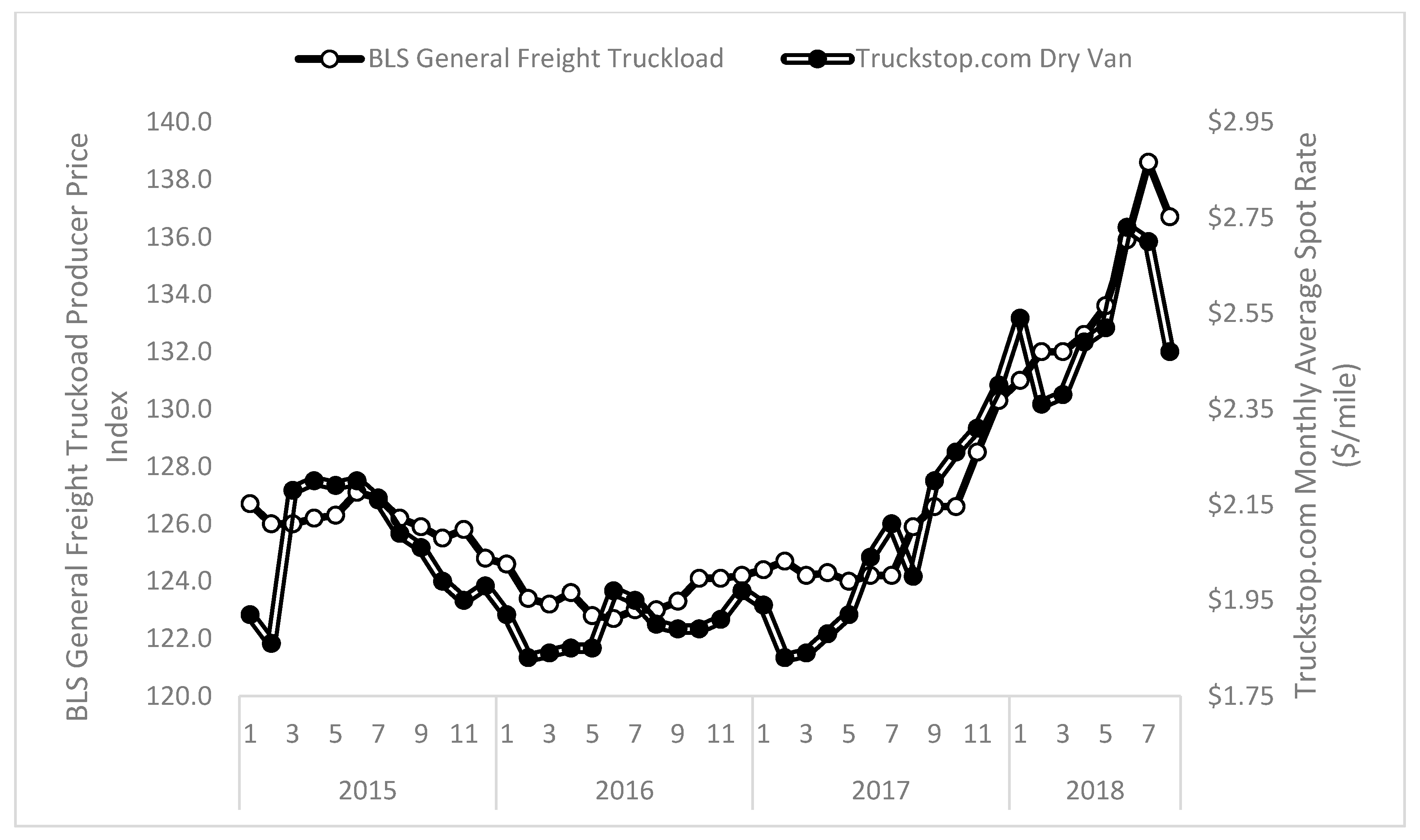
Figure 4.
Plot of month-over-month percent change for Trickload.BLS and DryVan.Truckstop.

Figure 5.
Model-implied forecast for Truckload.BLS for January 2014 through December 2018.

Figure 6.
Model-implied forecast for Truckload.BLS for February 2005 through December 2010.
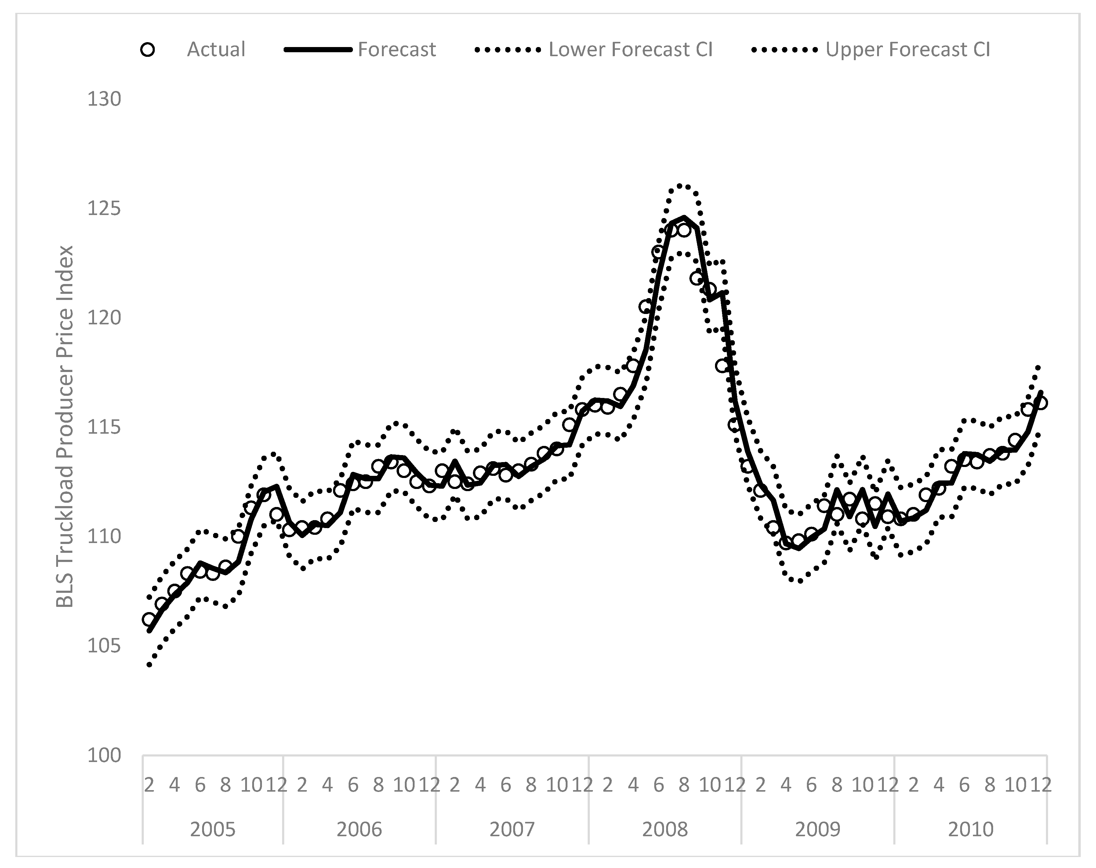
Figure 7.
Model-implied forecast for DryVan.Truckstop for February 2015 through December 2018.

Figure 8.
Model-implied forecast for Refrig.Truckstop for February 2015 through December 2018.
© 2018 by the author. Licensee MDPI, Basel, Switzerland. This article is an open access article distributed under the terms and conditions of the Creative Commons Attribution (CC BY) license (http://creativecommons.org/licenses/by/4.0/).
Share and Cite
MDPI and ACS Style
Miller, J.W. ARIMA Time Series Models for Full Truckload Transportation Prices. Forecasting 2019, 1, 121-134. https://doi.org/10.3390/forecast1010009
AMA Style
Miller JW. ARIMA Time Series Models for Full Truckload Transportation Prices. Forecasting. 2019; 1(1):121-134. https://doi.org/10.3390/forecast1010009
Chicago/Turabian StyleMiller, Jason W. 2019. "ARIMA Time Series Models for Full Truckload Transportation Prices" Forecasting 1, no. 1: 121-134. https://doi.org/10.3390/forecast1010009