Quantile Regression and Clustering Models of Prediction Intervals for Weather Forecasts: A Comparative Study

Abstract

Information about forecast uncertainty is vital for optimal decision making in many domains that use weather forecasts. However, it is not available in the immediate output of deterministic numerical weather prediction systems. In this paper, we investigate several learning methods to train and evaluate prediction interval models of weather forecasts. The uncertainty models of weather predictions are trained from a database of historical forecasts/observations. They are developed to investigate prediction intervals of weather forecasts using various quantile regression methods as well as cluster-based probabilistic forecasts using fuzzy methods. To compare and verify probabilistic forecasts, a novel score is developed that accounts for sampling variation effects on forecast verification statistics. The impact of various feature sets and model parameters in forecast uncertainty modeling is also investigated. The results show superior performance of the non-linear quantile regression models in comparison with clustering methods.

1. Introduction and Background

Deterministic Numerical Weather Prediction (NWP) models provide expected values of weather attributes on a three-dimensional spatial grid at certain forecast horizons [1]. These systems do not provide information about the uncertainty of the forecasts. However, there is always some level of error associated with point forecasts and therefore it is important to associate the forecast with an estimation of their expected uncertainty depending on different meteorological situations [2].

The knowledge of NWP forecast uncertainty is crucial in decision making and optimization processes involved in many applications. Wind power production [2,3,4,5,6,7,8], dynamic thermal rating of transmission lines [9,10,11,12,13], and extreme weather event prediction [14] are few applications where information about forecast uncertainty is often regarded as significant as the forecast values themselves [15,16]. In transmission line thermal rating applications, ambient temperature and wind data are used along with line current to determine the temperature of power conductors that limits the thermal capacity of the line. In this scenario, the decision of how much current can be passed through the transmission line cannot only rely on the deterministic weather forecasts. The knowledge of the weather forecast uncertainty is also crucial in maintaining the operation of the power grid within acceptable margins to account for the risk of conductor overloading and potential damage [17].

Prediction Intervals (PI) provide a range of values within which actual observations may lie with a certain degree of confidence [18,19,20], e.g., PI for ambient temperature may lie within [$3^{\circ }$, ${10}^{\circ }$] with a $95\%$ confidence. There is a large body of literature on calculating PIs from NWP models using ensemble forecasting systems [21,22,23]. However, forecast ensemble models incur large computational costs as they need to simulate a large number of scenarios for various numerical models with different initial conditions, making them infeasible in some applications. Specifically, for very short-term forecast applications where new information is made available with high frequency, ensemble forecasting is rather limited due to the computational burden imposed by rerunning an ensemble of heavy computational models. Additionally, availability of historical performance datasets for many forecast applications and existence of valuable uncertainty patterns in historical records have made post-processing an increasingly attractive approach to uncertainty modeling [20,24,25,26,27,28,29].

Different weather situations exhibit different levels of forecast uncertainty, and therefore different PIs can be found for different weather patterns discovered from the system performance records [2]. Clustering approaches and error distribution fitting methods have been used in a number of literary works [20,30] to train forecast uncertainty models from historical datasets. Cluster-based approaches present forecast uncertainty information as a full probability distribution of the target forecast using a single model. PIs at any desired level of confidence are then obtained from the fitted error distribution. In clustering-based PI computation, weather attributes and influential variables are used to cluster historical weather forecasts. Parametric (e.g., Gaussian) and non-parametric (e.g., empirical) distribution fitting models are employed to estimate the historical error distribution of each cluster. The developed statistical models determine the desired quantiles of new forecast dynamically. PIs for a future observation are calculated from the fitted error distribution of the cluster which the new forecast case belongs to.

In quantile regression based forecast uncertainty models, no distribution is assumed for the forecast error and each individual quantile is modeled independently [4,27,31]. Target quantiles are modeled as a function of influential feature sets through an optimization process. Various quantile regression methods have been developed and applied to weather data forecast uncertainty modeling [26,27,32]. The application of local quantile regression to obtain non-linear models of quantiles for wind power forecasts is proposed in [32]. In another study [27], additive quantile models are applied to model the quantiles of wind power forecast error. In both works [27,32], the resulting PIs are evaluated in terms of their inter-quantile range and actual observation frequencies compared to the forecasted quantile. However, in these works, the skill of the PI forecasting system is not evaluated in an objective framework. In another study [26], several statistical models including local quantile regression are used to obtain probabilistic wind power forecasts from NWP outputs. The quality of quantile forecasts is evaluated using sharpness and reliability measures instead of a forecast skill. A fuzzy inference system is proposed in [20] to model PIs of wind power generation. The fuzzy model is developed based on grouping of forecasts and a resampling technique is adopted for distribution fitting. A detailed comparative study on the quality of non-parametric probabilistic forecasts of wind power and their statistical performance is evaluated in [28]. It compares the fuzzy clustering based methods with the quantile regression-based approach in modeling PIs. An improved version of this approach is introduced in [30] where fuzzy clustering and error distribution fitting are applied to model the uncertainty of NWP forecasts. Time-adaptive kernel density estimation method for wind power forecasting is proposed in [24,25]. The model developed in [25] estimates the uncertainty of short-term wind power forecasts and the quality of the proposed model is benchmarked against a splines quantile regression model.

Despite the increasing attractiveness of the topic and large number of applications, there are only few studies in the literature that investigate a wide range of methods for forecast uncertainity modeling in practical settings [30,33,34,35]. The application of kernel quantile regression method [33] in learning non-linear uncertainty models and modeling weather forecast PIs is investigated in [34]. In this paper, a comprehensive study on the application of various quantile regression and cluster-based distribution fitting methods in modeling weather data uncertainty is conducted. A hybrid clustering-quantile regression approach is developed to mitigate the scalability limitation of non-linear kernel regression models. For forecast evaluation purposes, the developed PI models are applied to real-world datasets. Conclusive comparisons between PI forecasting systems is performed using a large real-world NWP dataset with a focus on “forecast skill” to compare and verify probabilistic forecast models accounting for sampling variation effects on forecast verification statistics. This approach also offers a good foundation to investigate the role of different parameters involved in such models. The variety and large size of the datasets used in this study compared to the previous studies in this domain also contribute to the significance of the empirical aspect of the study.

A number of literary works [36,37,38,39,40,41] have developed various measures of forecast skill. The evaluation of probabilistic predictions of scalar variables based on the continuous ranked probability score is investigated in [36]. In [37] a verification system has been developed for the ensemble prediction system based on the continuous ranked probability score. The importance of employing proper scores when selecting between various measures of forecast skill is explained in [38]. Bröcker [39] investigates the decomposition of proper scores into terms measuring the resolution and the reliability of a forecast. Multi-model ensemble combination prediction skill is investigated in [40]. Discrimination/ranking factor for ensemble forecasts is calculated in [41]. To the best of our knowledge, none of the previous works has incorporated the effect of sampling variations in their forecast evaluations. The scores developed in the existing studies [36,37,38,39,40,41] can be applied only in scenarios where both the predicted and target probabilities are provided in the form of full probability distributions.

Due to the limited availability of test samples, score measurements are subject to sampling variations. Therefore, it is crucial to assess the accuracy of observed skill when verifying the performance of forecasting systems. To evaluate PI forecast models, a forecast verification score is developed that considers the sampling effects on the forecast verification statistics. By decomposition and statistical analysis of the score measurements, we propose a model that considers sampling variations and uncertainties in the forecast evaluations, hence offering a more reliable comparison and evaluation of the PI forecast models.

This article brings several important contributions to the areas of weather forecasting and forecast uncertainty modeling. First, it presents a unique empirical and comparative study that covers a range of different cluster-based probabilistic models and quantile regression methods for modeling PIs of temperature and wind forecasts. It also develops a new hybrid clustering-quantile regression approach for PI modeling and evaluates its accuracy and performance. Last but not least, it proposes a novel forecast skill score which accounts for sampling variation effects.

The remainder of the text is organized as follows. Section 2 describes the basics of PIs and weather forecast uncertainty models including fuzzy-based clustering approach and various quantile regression models. The basic quality measures and the evaluation framework for PI forecasts are explained in Section 3. Section 4 provides experimental results and analysis of the quality of PIs obtained using different methods and parameter setups. Finally, the paper concludes with summarizing remarks and future directions in Section 5.

2. Weather Forecast Uncertainty Modeling

This section introduces different quantile regression and clustering methods that can be used to generate PIs for effective communication of forecast uncertainty.

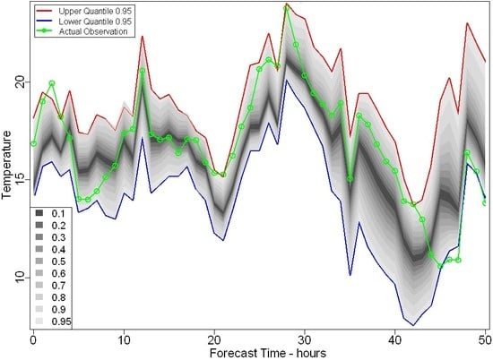
2.1. Prediction Intervals

Conditional PIs, as opposed to the static interval forecasting system, take different widths depending on the forecast context. Due to the random nature of forecast error, a forecast can be represented by a full probability distribution denoted as ${\widehat{f}}_{y_t|x}$ for the target attribute y at time t. Note that this distribution is conditional on x, representing the available information at the time of forecast. The uncertainty information of the forecast is represented by the spread of this distribution with more uncertain predictions exhibiting a wider spread. Any desired $\theta$ quantile is then obtained from this distribution [19]:

$$q_{y_t}^{\theta }=F_{y_t|x}^{-1}(\theta ),P(y_t<q_{y_t}^{\theta })=\theta$$

(1)

where $F_{y_t|x}$ is the cumulative distribution function of ${\widehat{f}}_{y_t|x}$. A $(1-\alpha )$-confidence level PI, $I_t^{\alpha }$, is defined by the lower and upper bound of PI that represent the range $[q_{y_t}^{{\theta }_l},q_{y_t}^{{\theta }_u}]$, where ${\theta }_l=\alpha /2$ and ${\theta }_u=1-\alpha /2$ [28]. The confidence level specifies the expected probability of the actual observation to be inside the PI range:

$$P(y_t\in I_t^{\alpha })=P(y_t\in [q_{y_t}^{{\theta }_l},q_{y_t}^{{\theta }_u}])=P(y_t\in [U_{y_t}^{\alpha },L_{y_t}^{\alpha }])=1-\alpha .$$

(2)

2.2. Prediction Interval Modeling Using Fuzzy Clustering

Different weather situations exhibit various levels of error [2]. The clustering approach is adopted to train clusters of forecast cases with a similar error behavior and develop PI models from weather data performance history. In fuzzy PI modeling, weather situations are defined as fuzzy sets using the training data. After past forecasts have been clustered, historical weather records are used to estimate the error distribution of each cluster. PIs at any desired level of confidence are then calculated from the distribution of forecast error at each cluster. Two attributes are considered to manually cluster forecast records into four fuzzy sets using wind power forecasting dataset in [20]. The empirical error distribution of a new forecast is then estimated using resampling.

Zarnani et al. developed several clustering algorithms to obtain groupings of weather situations using forecast attributes [30]. After clustering, parametric or non-parametric density estimation techniques are used to fit a probability distribution to the forecast error at each cluster. The authors also evaluated application of crisp and fuzzy clustering in modeling weather forecast uncertainty. In crisp clustering approach, each sample forecast is assigned to exactly one cluster. In fuzzy based clustering approach proposed in [20], each forecast sample is assigned to multiple clusters with different degrees of membership. Transitional weather regimes can be more effectively represented using fuzzy-based forecast uncertainty models. Fuzzy clustering is adopted to model forecast uncertainties in [30,35]. Published results confirm the high skill of PIs developed by error density estimation in fuzzy clustering models.

In this study, Fuzzy C-Means (FCM) clustering is used to model NWP forecast uncertainty and train PI models. Fuzzy patterns of historical forecasts are used to model the forecast error. This way, the forecast uncertainty modeled dynamically, based on various influential weather attributes. Groups of weather situations are discovered and their error distributions are modeled through clustering. PIs for a new forecast case are obtained from the trained model of the cluster which the new forecast belongs to. The intervals are then evaluated using verification measures described in Section 3. The process of uncertainty modeling for PI computation and evaluation using clustering based models is illustrated in Figure 1. The objective function of the clustering process takes the following form:

$$J={\mathrm{argmin}}_c\sum _{i=1}^N\sum _{j=1}^K{u}_{ij}^m{\parallel x_i-c_j\parallel }^2,$$

(3)

where m is the fuzzification factor, $c_j$ is the center of cluster j, and $u_{ij}$ represents the degree of membership of point $x_i$ in cluster j (${\sum }_{j=1}^K{u}_{ij}=1$).

2.3. Prediction Interval Modeling Using Linear and Non-Linear Quantile Regression

In this paper, a wide range of quantile regression models are developed to train forecast uncertainty models. In regression models, each individual quantile of a target variable is independently modeled as a linear/non-linear combination of a set of forecast attributes through an optimization process. In linear quantile regression model, $\theta$-quantile of the target variable y is estimated as a linear combination of influential variables denoted as $x^j$ [42,43]:

$${\widehat{q}}_y^{\theta }=f(x)={\beta }_0^{\theta }+{\beta }_1^{\theta }{x}^1+{\beta }_2^{\theta }{x}^2+\cdots +{\beta }_d^{\theta }{x}^d.$$

(4)

In modeling $\theta$-quantile of the traget attribute y, ${\beta }_y^{\theta }$ vector of quantile regression coefficients is estimated using the following objective function [31,42]:

$${\widehat{\beta }}_y^{\theta }={\mathrm{argmin}}_{\beta }\sum _{i=1}^N{L}_{\theta }(y_i-({\beta }_0^{\theta }+{\beta }_1^{\theta }{x}_i^1+{\beta }_2^{\theta }{x}_i^2+\cdots +{\beta }_d^{\theta }{x}_i^d)).$$

(5)

Linear programming techniques [42,43] are adopted to solve the optimization task using pairs of $(y_i$, $x_i)$ recorded in the historical dataset. The loss function of a $\theta$-quantile of target variable is defined as:

$$L_{\theta }({\delta }_i)=\left\{\begin{array}{c}\theta {\delta }_i{\delta }_i\ge 0\hfill \\ (\theta -1){\delta }_i{\delta }_i<0\hfill \end{array}\right.\mathrm{and}{\delta }_i=y_i-{\widehat{q}}_{y_i}^{\theta }.$$

(6)

The dataset of $(e_i,x_i)$ is used to model the lower and upper quantiles of target variable error, where $e_i$ represents the error of historical forecast case i, and x is the vector of influential variables. The $(1-\alpha )$-confidence level PI of target variable y for any new forecast sample of $x_{new}$ is estimated by the quantiles of error denoted as ${\widehat{\beta }}_e^{{\theta }_l}$ and ${\widehat{\beta }}_e^{{\theta }_u}$:

$${\widehat{I}}_{new}^{\alpha }=[{\widehat{q}}_{y_i}^{{\theta }_l},{\widehat{q}}_{y_i}^{{\theta }_u}],{\widehat{q}}_{y_i}^{{\theta }_l}=\langle {\widehat{\beta }}_e^{{\theta }_l},x_{new}\rangle +{\widehat{y}}_i,{\widehat{q}}_{y_i}^{{\theta }_u}=\langle {\widehat{\beta }}_e^{{\theta }_u},x_{new}\rangle +{\widehat{y}}_i,$$

(7)

where $\langle .,.\rangle$ represents inner product of the two vectors. As opposed to the cluster-based models described in Section 2.2, in quantile regression methods new models need to be trained for each level of confidence.

A transformation basis function, $\mathsf{\Phi }(x)$, can be developed to derive new features from the available feature sets. The PI modeling methods that use the transformed features are referred to as Non-Linear Quantile Regression (NLQR). In non-linear regression models, the non-linear relationships between target variable and the new explanatory variables is optimized to model the forecast quantiles using the formulation described in (5).

2.3.1. Quantile Regression with Spline-Basis Functions

To train non-linear models of weather forecast quantiles, spline-basis functions [25,43] provide the non-linear transformation of influential attributes to model forecast quantile non-linear models [44]:

$${\widehat{q}}_y^{\theta }={\beta }_0^{\alpha }+\sum _{j=1}^d\sum _{k=1}^{d{f}_j}{\beta }_{j,k}^{\theta }{f}_{j,k}(x^j),$$

(8)

where $f_{j,k}$ is the spline basis function with $d{f}_j$ degrees of freedom, determined by running experiments on the training dataset. The regression model is then optimized by the linear optimization task formulated in (5).

2.3.2. Local Quantile Regression

In Local Quantile Regression (LocQR) models a linear relationship between the target quantile and influential features is estimated in the close neighborhood of the explanatory variables of $\mathrm{x}$. In LocQR models forecast intervals are modeled by considering a set of training samples centered around $\mathrm{x}$ [45]:

$${\widehat{\beta }}_{e,\mathrm{x}}^{\theta }={\mathrm{argmin}}_{\beta }\sum _{i=1}^N{L}_{\theta }(y_i-{\beta }^{\theta }({\mathrm{x}}_i-\mathrm{x}))W({\mathrm{x}}_i,\mathrm{x}).$$

(9)

Forecast quantile of a new forecast case $\mathrm{x}$ is estimated using the closest training examples in the feature space. Forecast quantiles are weighted based on the distance of $\mathrm{x}$ to its $\lambda N$-th nearest neighbour in the training sample ${\mathrm{x}}_{1\cdots N}$ [32]. Using LocQR, as opposed to other regression models, in order to estimate the forecast quantiles for each new forecast case $\mathrm{x}$, new regression models need to be optimized at that specific point $\mathrm{x}$.

2.3.3. Kernel Quantile Regression

To train non-linear models of weather forecast quantiles, the optimization process involved in regression models can be performed in Reproducing Kernel Hilbert Space (RKHS). Kernel Quantile Regression (KQR) [33] is a non-parametric regression to estimate forecast quantile non-linear models. To model the $\theta$-quantile of the target variable y using KQR, the ${\beta }_y^{\theta }$ vector of quantile regression coefficients is estimated using the following objective function:

$${\widehat{\beta }}_y^{\theta }={\mathrm{argmin}}_{\beta }C\sum _{i=1}^N{L}_{\theta }(y_i-{\beta }^{\theta }x)+\frac{1}{2}{\parallel \beta \parallel }_{\mathcal{H}}^2,$$

(10)

where $\mathcal{H}$ denotes a RKHS on $\mathrm{x}$, and the cost factor C accounts for the total loss over the penalization of overfitting. The last term is the regularizer applied to penalize complex functions and avoid overfitting. A dual form of the optimization problem can be obtained using Lagrange multipliers method that represents the model by vector of weights (${\alpha }_i,i=1\cdots N$) over sample space rather than features in the primal problem [46]:

$$\begin{array}{c}{\widehat{\alpha }}_y^{\theta }={\mathrm{argmin}}_{\alpha }\frac{1}{2}{\alpha }^{T}K\alpha -{\alpha }^T\overrightarrow{y},\\ \mathrm{subject}\mathrm{to}C(\theta -1)\le {\alpha }_i\le C\theta ,1\le i\le N,\\ {\overrightarrow{1}}^T\alpha =0,\end{array}$$

where K is the kernel matrix obtained from $K_{ij}=k(x_i,x_j)=\langle \mathsf{\Phi }(x_i),\mathsf{\Phi }(x_j)\rangle$, k is the corresponding kernel function which provides $\mathsf{\Phi }$-mapping of inputs into a new feature space, $\mathsf{\Phi }(x)$ is the corresponding feature map of x, and $\alpha$ is the vector of Lagrange multipliers. A common choice for the kernel function is Gaussian kernel [46] defined as $K_{ij}=\exp (-\parallel x_i-x_j{\parallel }^2/2{\sigma }^2)$, where $\sigma >0$ is the kernel width parameter which needs to be tuned. In this study, other choices for the kernel function are experimentally tested as well.

Due to the low scalability (high dimensionality) of the kernel quantile based models, the training data is first clustered into a number of partitions using the feature set available for weather forecast uncertainty modeling. In the second step, the kernel quantile regression algorithm is applied independently to each partition to train two non-linear quantile models, one for the lower quantile and another model for the upper quantile. To verify the model, a new forecast is first assigned to its nearest cluster and then the quantile model trained for that cluster is used to estimate the quantiles for the new forecast case. The developed hybrid clustering-KQR model has the highest computation cost compared to other approaches. Experiments for the choice of clustering algorithm and number of clusters are performed to fine tune the final output uncertainty model using KQR.

3. An Evaluation Framework for Prediction Interval Forecasts

In this section, various measures for evaluation of the quality of PI computation methods are discussed. Reliability, sharpness, and resolution are introduced as the main attributes for the assessment of PI models. A novel score is developed to evaluate the quality of PI computation methods by taking sampling variation into account.

3.1. Basic Verification Measures

To model forecast uncertainties, some methods estimate the full probability distribution of the target attribute while only a PI is considered in other models [28,47,48]. To evaluate the probabilistic PI forecasts, some basic verification measures are widely used in the literature [26,28,49]. Reliability and sharpness are basic quality measures for evaluating PI forecast models. Reliability measures the ability of the forecasting system to provide PIs that represent their associated confidence level in test experiments [20]. Reliability of PI forecast system in test scenarios for PIs with confidence level of $1-\alpha$ is defined as follows:

$$\begin{array}{cc}\hfill & Re{l}^{\alpha }={\overline{\xi }}^{I^{\alpha }}-(1-\alpha ),\mathrm{where}{\overline{\xi }}^{I^{\alpha }}=\frac{1}{N_T}\sum _{i=1}^{N_T}{\xi }_i^{I^{\alpha }}\hfill \end{array}.$$

(11)

The indicator variable ${\xi }_i^I$ tells if the actual outcome lies (“hit”) or not (“miss”) in the estimated PI. According to the above equation, the reliability measure indicates the percent of actual observation in the $N_T$ test samples that falls inside the PI.

The sharpness measure of probabilistic forecast models corresponds to the average width of PIs estimated by a forecast uncertainty model. This measure demonstrates the ability of forecasting systems to make predictions with lower uncertainty [20,27]:

$$Sh{p}^{\alpha }={\overline{Width}}^{\alpha }=\frac{1}{N_T}\sum _{i=1}^{N_T}({\widehat{q}}_{y_i}^{{\theta }_u}-{\widehat{q}}_{y_i}^{{\theta }_l})=\frac{1}{N_T}\sum _{i=1}^{N_T}({\widehat{U}}_i^{\alpha }-{\widehat{L}}_i^{\alpha }).$$

(12)

The resolution measure corresponds to the ability of PI forecasting system to provide a situation-dependent assessment of the uncertainty. It is defined as the standard deviation (variation) of the width of PIs:

$$Re{s}^{\alpha }={\left[\frac{1}{N_T-1}\sum _{i=1}^{N_T}{({\widehat{U}}_i^{\alpha }-{\widehat{L}}_i^{\alpha }-Sh{p}^{\alpha })}^2\right]}^{\frac{1}{2}}.$$

(13)

3.2. Skill Score for Evaluating Prediction Interval Forecast Models

For the purpose of comparing the quality of various interval forecasting models, Root Mean Squared Error (RMSE) only considers centers of the forecast intervals but ignores their boundaries (forecast uncertainty magnitudes). In this paper a novel score is developed that compares different PI forecasting models. The developed score incorporates PI boundaries in estimating forecast quality:

$$SScore=-\sum _{i=1}^{N_T}[({\xi }_i^{{\widehat{L}}_{y_i}^{\alpha }}-{\theta }_l)(y_i-{\widehat{L}}_{y_i}^{\alpha })+({\xi }_i^{{\widehat{U}}_{y_i}^{\alpha }}-{\theta }_u)(y_i-{\widehat{U}}_{y_i}^{\alpha })],$$

(14)

where ${\xi }_i^q$ is equal to one if $y_i\le q$, and zero otherwise. This scoring rule is negatively oriented, i.e., smaller values are preferred as an error measure, and admits a maximum value of 0 for perfect probabilistic predictions. In this measure, uncertain forecasts with wide PIs and missed observations are penalized by the magnitude equal to their distance from the interval boundaries [27,28,32,50]. The skill score as defined above is “strictly proper” [38,51] and gives the optimal score to a forecast whose PI follows the true distribution of the target [38]. Details of the mathematical definitions and proofs can be found in [51]. It should be noted that while the term “skill score” here is used as a synonym for “score”, skill scores are occasionally referred to as specific relative scores for the comparison of predictive performances relative to a reference forecast in the atmospheric sciences [51,52].

The skill score defined in (14) can be simplified by considering several possible scenarios:

• when a “hit” occurs for forecast PI of case i, then $({\xi }_i^{{\widehat{L}}_{y_i}^{\alpha }},{\xi }_i^{{\widehat{U}}_{y_i}^{\alpha }})=(0,1)$; by substituting the values in (14) we have $SScor{e}_i(hit)=-\frac{\alpha }{2}({\widehat{U}}_{y_i}^{\alpha }-{\widehat{L}}_{y_i}^{\alpha })=-\frac{\alpha }{2}{\overline{Width}}_i^{\alpha }$
• in the case of a “missed” observation appearing either on the right or the left side of the PI boundaries, the values of $({\xi }_i^{{\widehat{L}}_{y_i}^{\alpha }},{\xi }_i^{{\widehat{U}}_{y_i}^{\alpha }})$ are equal to $(0,0)$ or $(1,1)$, respectively.

  −

  when it is on the right side, it has a positive distance of ${\delta }_i$ from the upper boundary ${\widehat{U}}_{y_i}^{\alpha }$; by substituting these values we have $SScor{e}_i(rightmiss)=-\frac{\alpha }{2}{\overline{Width}}_i^{\alpha }-{\delta }_i$.

  −

  when it is on the left side, an equal score is obtained.

As the overall miss rate is $(1-{\overline{\xi }}^{I^{\alpha }})$, the skill score obtained by a PI forecasting system over $N_T$ test cases is defined as:

$$SScore=-N_T({\theta }_l{\overline{Width}}^{\alpha }+(1-{\overline{\xi }}^{I^{\alpha }}){\overline{\delta }}^{\alpha })=-N_T(\frac{\alpha }{2}{\overline{Width}}^{\alpha }+{\overline{\Delta }}^{\alpha }),$$

(15)

where ${\overline{\Delta }}^{\alpha }$ is the average distance of observations from the PI boundaries. It is calculated as the mean of ${\Delta }_i$ values for test cases $i=1\cdots N$. For test case i, ${\Delta }_i$ is equal to zero for a hit, and ${\delta }_i$ for a miss, where ${\delta }_i$ is defined as the distance of observation from the boundaries. The sample statistic ${\overline{\Delta }}^{\alpha ,j}$ measured in a cluster with fewer test cases has higher uncertainty compared to the case where it is measured in another cluster with larger test cases. Therefore, the statistic ${\overline{\Delta }}^{\alpha }$ is subject to sampling variations. This sampling variation is caused by the limited number of test samples and it makes the skill score measurements uncertain. An uncertainty analysis needs to be performed to incorporate sampling variation impact on forecast evaluation process.

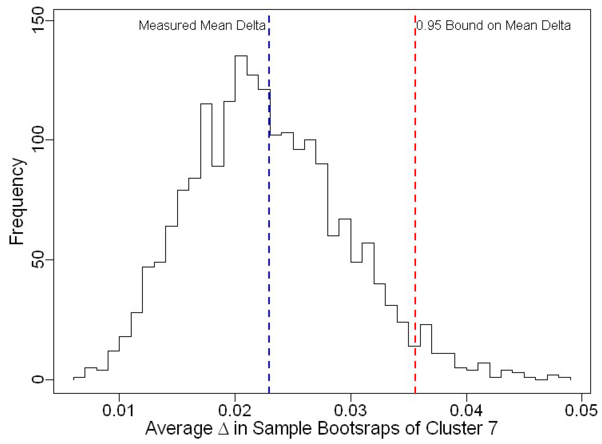
3.3. Uncertainty of Skill Score Measurements

The impact of sampling variations on forecast verification statistics is significant in weather forecast verification studies [15]. In this study a novel skill score is developed that models the uncertainty of skill score measurements accounting for sampling variations.

In cluster-based PI models introduced in Section 2.2, after partitioning feature space into K clusters, the skill score in each cluster is independently estimated using the test cases that belong to that specific cluster. The overall score of the PI forecast system is estimated as the weighted average of the skill scores calculated in each cluster. Also, in quantile regression based models, the forecast records are clustered into a numbers of groups to analyze the skill score sampling variations and estimate confidence bound. Therefore, the terms ${\overline{Width}}^{\alpha }$ and ${\overline{\Delta }}^{\alpha }$ are estimated as the weighted sum of their measured values in K clusters, with $N_{T_j}$ test cases in each cluster j:

$$\widehat{SScore}=-N_T(\frac{\alpha }{2}{\overline{Width}}^{\alpha }+{\overline{\Delta }}^{\alpha })=-\sum _{j=1}^K\left|N_{T_j}\right|(\frac{\alpha }{2}{\overline{Width}}^{\alpha ,j}+{\overline{\Delta }}^{\alpha ,j})$$

(16)

In the case of PI models based on clustering, each cluster ($j=1,\dots ,K$) is independently evaluated using the $N_{T_j}$ test cases that actually belong only to that cluster. Finally, a weighted average of the K skill scores yields the overall score of the method. It is plausible that the sample statistic ${\overline{\Delta }}^{\alpha ,1}$ measured in a cluster with fewer test cases (e.g., $N_{T_1}=100$) has higher uncertainty compared to the same statistic ${\overline{\Delta }}^{\alpha ,2}$ in a cluster measured using more test cases (e.g., $N_{T_2}=4000$). To obtain a $\beta$-confidence bound on skill score with a desired level of confidence, the sampling distribution of ${\overline{\Delta }}^{\alpha ,j}$ is estimated by bootstrapping technique in each cluster j [53]. The $\beta$-quantile of the ${\overline{\Delta }}^{\alpha ,j}$ statistic is then estimated as a one-sided confidence interval denoted as ${\overline{\Delta }}^{\alpha ,j^{\beta }}$. Using Equation (15) the $\beta$-confidence bound over skill score is obtained as $SScor{e}^{\beta }$:

$$P({\overline{\Delta }}^{\alpha ,j}<{\overline{\Delta }}^{\alpha ,j^{\beta }})=\beta ,P(SScore>SScor{e}^{\beta })=\beta .$$

(17)

According to [51], the bootstrap-based skill score is considered to be a proper score. A $95\%$ confidence bound is deemed to find the confidence interval over ${\overline{\Delta }}^{\alpha ,j}$ using 2000 bootstrap samples. Figure 2 presents an example of sampling distribution of ${\overline{\Delta }}^{\alpha ,7}$ and its confidence bound for a sample cluster of test cases estimated using quantile regression model with spline-basis functions.

As previously described, the reliability/coverage measure for PI forecasters suggests that the empirical coverage of observations in a test setting is comparable to the required confidence level. In this study, the $95\%$ confidence lower bound of the coverage measure is calculated to account for sampling variation in the verification of PI forecasts. As indicated by the Binomial test, a cluster with $90\%$ coverage (hit rate) in 1000 test cases has a greater lower bound (i.e., Coverage${}^{0.95}=88.3\%$) when compared to a cluster with $90\%$ coverage in 200 test samples (i.e., Coverage${}^{0.95}=85.8\%$). Also, the $SScor{e}^{0.95}$ measure is used to verify different forecast uncertainty models by considering sampling uncertainties in test experiments. The overall performance of a PI forecast model is evaluated by the skill score measure. For further details on the importance of the uncertainty analysis refer to [30].

4. Evaluation Study

The developed clustering and regression based approaches for modeling NWP forecast uncertainty are used to train PI models from performance history. The quality and accuracy of the resulting interval forecasts are measured using the proposed evaluation framework.

4.1. Data and Models

The performance of cluster-based and quantile regression-based uncertainty models in obtaining PI forecasts from numerical weather forecasting model is evaluated through experimental studies. The dataset is obtained from the Weather Research and Forecasting (WRF) model with the resolution of one hour. The WRF $v3$ simulations are run in three nested grids with the resolutions of $10.8$ km, $3.6$ km, and $1.2$ km. Weather observations at the same time and location as the WRF model are also obtained from the National Center for Atmospheric Research (NCAR) data repository.

PI modeling experiments are based on $51,000$ records of historical data, each containing 35 features. The dataset covers three years (2007–2009) of weather records collected two meteorological stations in the cities of Hope and Agassiz in the province of British Columbia, Canada. A second NWP dataset of 13,000 records contains hourly temperature and wind speed forecasts at 60 stations in BC, Canada for summer 2009. For this dataset, forecast uncertainty models are developed using 10 available features. Due to the similarity of results obtained using the two datasets and the larger size of the first set, only the results for the first dataset are reported here.

Influential features extracted from the first dataset for PI modeling include ambient temperature ($t2$, measured at 2 m), wind speed and direction ($ws$ and $wd$, at 10 m), surface pressure ($sp$), dew temperature ($dt$), relative humidity ($rh$), hour of day (h), day (d) and month of year (m), and weather station identification. The set of features containing the above variables is referred to as the basic feature set. In addition, predicted temperature, horizontal and vertical wind speed and wind direction for different pressure levels of 500, 700, 850, 905, and $950millibar$ are considered, referred to as the pressure level feature set. To take the temporal aspects of weather situations into account, additional features are derived from the gradient of surface pressure between the current forecast and the forecasts of 1, 3, 6, and 12 h ahead, denoted as pg1, pg3, pg6, and pg12. To identify the best predictor attributes of uncertainty, the $95\%$ PI model of temperature forecasts is estimated with different feature sets. Table 1 describes seven different combinations of the basic features and pressure tendency. Table 1 lists several extended feature sets that include pressure level attributes. In addition, dimensionality of some large feature sets is reduced using the most significant components obtained through Principal Component Analysis (PCA).

For the evaluation of various PI forecasting models, the available dataset is split into a training set and a test set. In all models the dataset is normalized using standardized anomaly technique based on the training set. To validate the trained models developed using cluster-based and regression models, three-fold cross validation is performed by splitting different years into folds; two years of data is used to train the forecast uncertainty models and PIs for the third year is obtained using the trained model and evaluated for the quality. Performing a random-based K-fold cross validation yields the same result and therefore only three-fold cross validation results are reported here.

To allow comparison of various uncertainty models, several baseline models are developed. A climatological model computes PIs considering the entire forecast history ($K=1$). Also, two other baseline models are developed using manual categorization of forecast records based on a categorizing attribute; one based on forecast month ($K=12$) and another one based on forecast temperature ($K=10$).

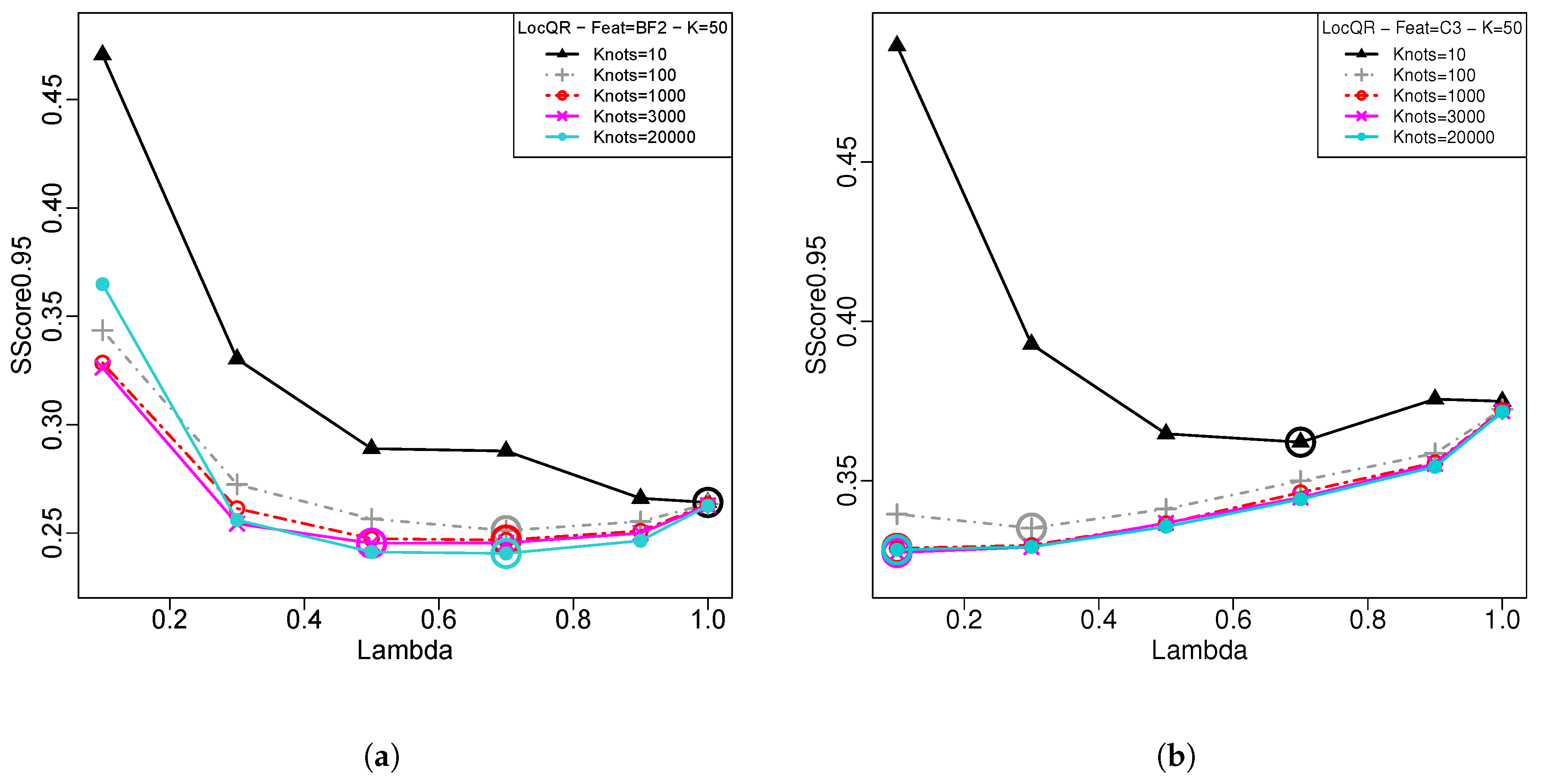
4.2. Comparative Analysis of the PI Forecast Models

For the clustering-based approach, various models are developed based on different combination of feature set (as listed in Table 1), fitting method (Gaussian, Weibull, Empirical, and Kernel density smoothing), clustering algorithm (K-means, CLARA, and FCM) and number of clusters (K). Results from an earlier study [30] confirm that the proposed FCM clustering approach achieves forecast PIs with higher skill compared to other clustering-based and baseline models. The fuzzification factor and number of clusters in the FCM model are experimentally tuned to the values of $1.2$ and 45, using grid search as suggested in [30].

In quantile regression models, the forecast records are grouped into a number of clusters between 2 and 100 to analyze the skill score sampling variations in these subspaces and to estimate its confidence bounds. In quantile regression approaches the upper and lower quantile models are trained independently. As a result there may be cases where the upper and lower quantiles overlap and do not conform to each other. These exceptional cases are substituted by the climatological baseline PI model to provide a balanced comparison among all models.

Figure 3a depicts the impact of the number of degrees of freedom on the skill score of the Spline-based Quantile Regression (SPQR) models when using different feature sets. Different curves represent the variation of $SScor{e}^{0.95}$ over different feature sets when the number of clusters is equal to $K=50$. The number of clusters is selected in a way that best represents the groups of weather situations in the clustering-based models. In this figure, the degree of freedom by which the best score is achieved for SPQR model is encircled. It is noticeable that feature sets BF2 and BF2PG provide the best PIs for SPQR models. Figure 3b demonstrates the impact of the number of degrees of freedom on the skill score of SPQR models when using different number of clusters. This figure shows that the SPQR model with four degrees of freedom consistently provides the best skill score regardless of the numbers of clusters used for analyzing the skill score sampling variations.

In LocQR model, the PI evaluation process requires a relatively long computational time as the upper and lower quantile models are trained for each new forecast test case. Therefore, LocQR models are trained for a specific number of points randomly selected from the training samples. The LocQR model trained for the nearest knot to the new test case is applied to estimate the PIs for each new forecast case. The performance of the LocQR forecast uncertainty model is investigated by considering the role of kernel radius, $\lambda$, and different numbers of knots. Two feature sets of BF2 and C3 are considered in the experiments for computing skill score of PI models estimated using LocQR. Figure 4 indicates that, when BF2 feature set is used to train the PI models, the best skill score is achieved for $\lambda =0.7$. BF2 feature space has higher dimension and therefore a larger neighborhood is required for the local model to efficiently learn forecast uncertainties. However, when using the lower dimensional feature space of C3, $\lambda =0.1$ will provide the best skill score for LocQR models. Results also confirm that using a lower number of knots (e.g., 3000), the PI models can achieve comparable accuracies with higher computational efficiency.

To handle the large size of the kernel matrix in KQR models, the Cholesky decomposition [24] is applied to the kernel matrix to reduce its rank. Also, to address the high dimensionality of KQR models, the training data is first clustered into K partitions based on the influential attributes used in the model. KQR models are then trained for each partition independently. Results from the experiments confirm that the quality of PI forecast is optimized when K-means clustering with 10 clusters is applied to train hybrid clustering-KQR models. In KQR forecast uncertainty models, different choices for kernel function are experimentally tested. Gaussian kernel compared to other alternative choices results in an improved quality and skill of PI forecasts. The kernel parameters of $\sigma$, i.e., kernel width, and C, i.e., the position of the center of the peak, must be tuned. The skills of PIs over options for parameters $\sigma$ and C are represented in Figure 5a. To evaluate the impact of various feature attributes on the quality of temperature PI forecasts of the trained KQR models, box plots of skill scores are presented in Figure 5b. As can be seen in this figure, the two feature sets BF2 and BF2PG provide PI forecast models with higher quality. These two feature sets include wind speed components at five pressure levels that contain information about the level of instability of the forecast atmospheric situation. This information can be very helpful for the uncertainty models to achieve higher skill. Among the basic feature sets, C3 has the best score, suggesting that the attributes of temperature, wind speed, and hour-of-day are the key features in the uncertainty models. It is also observed in the experiments that PIs of KQR models applied to lower dimensional feature sets, e.g., BF1 or C3, have higher skills compared to other forecast uncertainty models. For example, a set of experiments reveals that $SScor{e}^{0.95}=0.3006$ is achieved by KQR model while a $SScor{e}^{0.95}$ of $0.3359$ is obtained from SPQR approach when these models are applied to BF1. This demonstrates the higher competency of KQR models in handling lower dimensional quantile learning problems due to the hybrid nature of the learning process involved.

Figure 6b presents sample temperature PIs with various confidence levels along with observations in a station obtained from the best SPQR model with four degrees of freedom. It is important to note that these variations in the forecast uncertainty are learned using historical statistical information of the different weather situations.

The PI quality measures based on three-fold cross validation for FCM clustering based and quantile regression models are presented in

Table 2. PI verification measures for top models of different methods based on three-fold (yearly) cross validation.

Algorithm	K	Features	Fit/Params	Sharpness (${}^{\circ }$C)	Coverage (%)	Coverage${}^{0.95}$ (%)	Resolution	RMSE	SScore	SScore${}^{0.95}$
SPQR	50	BF2	$df=4$	$6.68$	$93.56$	$91.10$	$1.76$	$1.92$	$0.2125$	$0.2323$
LocQR	50	BF2	$\lambda =0.7$	$6.92$	$93.46$	$90.97$	$1.73$	$2.00$	$0.2202$	$0.2406$
NLQR	50	BF2	-	$6.92$	$93.15$	$90.62$	$1.79$	$2.00$	$0.2264$	$0.2492$
KQR	50	BF2	$\sigma =0.0042$ $C=4$	$7.16$	$93.09$	$91.51$	$1.85$	$2.05$	$0.2362$	$0.2561$
LQR	50	BF2PG	-	$7.91$	$94.39$	$92.05$	$1.64$	$2.17$	$0.2438$	$0.2640$
FCM	45	BF2	Kernel	$10.62$	$94.89$	$92.77$	$1.59$	$2.77$	$0.3220$	$0.3432$
Base-Month	12	Month	Kernel	$12.21$	$95.12$	$94.10$	$1.91$	$3.12$	$0.3601$	$0.3704$
Base-Temp.	10	Normal	Temp.	$11.70$	$94.44$	$93.57$	$0.98$	$3.04$	$0.3620$	$0.3725$
Base-Clim.	1	-	Normal	$12.17$	$94.78$	$94.49$	$0.00$	$3.11$	$0.3740$	$0.3774$

. The best model set up for various quantile regression, clustering-based, and baseline models along with the basic quality measures are reported in this table. For the purpose of point forecast evaluation, the median of each PI is considered as the point forecast of the trained model. This forecast is calibrated based on the historical patterns in the forecast accuracy records. The performance of point forecasts of the uncertainty models are evaluated using RMSE measure. Results confirm that the point forecasts obtained from the trained uncertainty models have significantly higher performance when compared to baseline models. This can be attributed to the fact that, in the learning-based models, the median of the forecast error is modeled using the influential attributes. This can be considered as dynamic elimination of forecast bias in these models. The results of this study also conform to the results discussed in [28], however, the improvement obtained using quantile regression models over clustering based models is considerably greater in the experiments reported here.

Experimental results reveal that all PI models developed using learning methods surpass the baseline models ($p<0.0005$). Results confirm the higher quality of PI forecasts estimated by quantile regression models compared to the cluster-based models. The best PI forecast models are obtained from the SPQR model with four degrees of freedom using BF2 feature set. It is followed by LocQR, NLQR, KQR, and LQR. All these quantile regression models outperform the best fuzzy clustering based method with 45 clusters and kernel density smoothing in terms of $SScor{e}^{0.95}$. Empirical width distribution of the forecasted $95\%$ PIs using different uncertainty models is depicted in Figure 6a where horizontal line shows the best baseline model. The figure shows that quantile regression models, compared to the FCM clustering model, provide relatively sharper PI forecasts.

The impact of number of clusters on SScore${}^{0.95}$ for different quantile regression models is depicted in Figure 7. This figure also confirms that the PIs obtained by SPQR models have higher quality and skill compared to other models. For LocQR models, the model with $\lambda =0.5$ has a higher skill score compared to $\lambda =0.7$ without considering sampling variation. However, when the sampling variations are taken into account in $SScor{e}^{0.95}$ using higher number of clusters, the model with $\lambda =0.7$ gets a higher skill score confidence bound. The misleading initial ranking when using skill score only is most likely due to the fact that the model provides good PIs in the areas that insufficient samples are available to reliably evaluate the quality of the PIs. This example signifies the role of skill score uncertainty analysis in PI evaluations.

4.3. PI Forecast Evaluation Results

For the evaluation of various PI forecasting models, the trend of Reliability and Reliability${}^{0.95}$ for different levels of confidence is depicted in Figure 8. For the specific confidence levels of $0.1$, $0.5$, and $0.95$ the observed coverage measure of various PI forecast models is presented in

Table 3. Detailed coverage and miss ratio observations in test for three confidence levels.

	$(1-\mathit{\alpha })=0.95$				$(1-\mathit{\alpha })=0.5$				$(1-\mathit{\alpha })=0.1$
Algorithm	Avg.$\delta$ (${}^{\circ }$C)	Miss (Left)%	Hit (Center)%	Miss (Right)%	Avg.$\delta$ (${}^{\circ }$C)	Miss (Left)%	Hit (Center)%	Miss (Right)%	Avg.$\delta$ (${}^{\circ }$C)	Miss (Left)%	Hit (Center)%	Miss (Right)%
SPQR	0.70	3.3	93.6	3.2	1.06	25.8	48.9	25.3	1.35	45.5	9.9	44.6
LocQR	0.75	3.4	93.5	3.2	1.11	26.8	49.2	24.0	1.41	46.8	10.0	43.2
NLQR	0.78	3.4	93.2	3.4	1.12	25.8	48.9	25.3	1.42	45.3	10.0	53.7
KQR	0.82	3.4	93.1	3.5	1.20	28.4	46.2	25.4	1.55	46.3	11.2	42.5
LQR	0.82	2.8	94.4	2.9	1.22	25.2	49.7	25.1	1.55	45.1	10.0	54.0
FCM	1.08	2.7	94.9	2.4	1.62	24.8	50.3	24.9	2.03	44.9	10.0	45.2
Base-Month	1.11	2.5	95.1	2.4	1.82	24.6	50.7	26.6	2.32	44.8	10.3	44.9

. It also reports $\overline{\delta }$, i.e., the average distance of an observation from PI boundaries among the missed cases as defined in Section 3.2. The average width of PIs estimated using various forecast uncertainty models at different levels of confidence is presented in Figure 9a. The average distance of observations from PI boundaries, i.e., ${\overline{\Delta }}^{\alpha }$, over the selected range of confidence levels estimated by various PI forecast models is projected in Figure 9b. Figure 10 compares the overall skill score of various PI forecasting models at different confidence levels. Results indicate that the PIs estimated using SPQR model, compared to other forecast uncertainty models, achieve higher quality in terms of sharpness, reliability, and overall skill score.

The main difference between quantile regression and clustering based methods in modeling forecast uncertainty is that, unlike quantile regression models, the forecast error information is not directly incorporated in the optimization process involved in the cluster-based models. More specifically, the quantile of forecast error in regression models is directly estimated using a regression model that relates the forecast error to the influential attributes. The parameters of the regression model are then fine-tuned by incorporating forecast error information in the optimization process. However, in cluster-based models, clusters of weather data historical records are first trained based on forecast weather situations without considering forecast errors. After clustering of forecast samples is completed, error density model in each cluster is estimated using the distribution fitting process. This evidences the superior performance of quantile regression models compared to clustering-based forecast uncertainty models.

5. Conclusions

This article introduced several new uncertainty models developed to extend the usefulness of NWP forecasts through PIs. The models are based on various quantile regression techniques, a new hybrid kernel quantile regression method, and several clustering approaches. To measure the quality and accuracy of the various PI models, a new evaluation framework that considers the impact of sampling variations has also been developed. The proposed PI forecasting models can be used in real world applications to enhance point forecasts of NWP systems with information on prediction uncertainty.

The results of conducted computational experiments bring some interesting insights into the nature of individual approaches, including the impact of different model parameters and the selection of features. Although clustering-based models have a marginally higher reliability, the results demonstrate the superior performance of quantile regression models, especially the spline quantile regression model, in terms of overall forecast skill. Cluster-based approaches model the entire probabilistic distribution of a forecast in a single model, while quantile regression models need to be updated for each new forecast case.

Development and application of kernel expansion functions to obtain non-linear quantile regression models is a promising direction for future research in atmospheric uncertainty modeling. The use of time series based methods for PI modeling can also be considered. A very interesting future direction would be to combine predictions from multiple trained models in an ensemble to further improve the accuracy [54].

References

1. The Weather Research and Forecasting (WRF) Model. Available online: http://www.wrf-model.org/index.php (accessed on 21 July 2017).
2. Lange, M. Analysis of the Uncertainty of Wind Power Predictions. Ph.D. Thesis, Universität Oldenburg, Oldenburg, Germany, 2003. [Google Scholar]
3. Pinson, P. Estimation of the Uncertainty in Wind Power Forecasting. Ph.D. Thesis, École Nationale Supérieure des Mines de Paris, Paris, France, 2006. [Google Scholar]
4. Wan, C.; Lin, J.; Wang, J.; Song, Y.; Dong, Z.Y. Direct quantile regression for nonparametric probabilistic forecasting of wind power generation. IEEE Trans. Power Syst. 2017, 32, 2767–2778. [Google Scholar] [CrossRef]
5. Andrade, J.R.; Bessa, R.J. Improving Renewable Energy Forecasting with a Grid of Numerical Weather Predictions. IEEE Trans. Sustain. Energy 2017, 8, 1571–1580. [Google Scholar] [CrossRef]
6. Huang, C.M.; Kuo, C.J.; Huang, Y.C. Short-term wind power forecasting and uncertainty analysis using a hybrid intelligent method. IET Renew. Power Gener. 2017, 11, 678–687. [Google Scholar] [CrossRef]
7. Iversen, E.B.; Morales, J.M.; Møller, J.K.; Madsen, H. Short-term probabilistic forecasting of wind speed using stochastic differential equations. Int. J. Forecast. 2016, 32, 981–990. [Google Scholar] [CrossRef]
8. Juban, R.; Ohlsson, H.; Maasoumy, M.; Poirier, L.; Kolter, J.Z. A multiple quantile regression approach to the wind, solar, and price tracks of GEFCom2014. Int. J. Forecast. 2016, 32, 1094–1102. [Google Scholar] [CrossRef]
9. Hosek, J.; Musilek, P.; Lozowski, E.; Pytlak, P. Effect of time resolution of meteorological inputs on dynamic thermal rating calculations. IET Gener. Transm. Distrib. 2011, 5, 941–947. [Google Scholar] [CrossRef]
10. Pytlak, P.; Musilek, P.; Lozowski, E.; Toth, J. Modelling precipitation cooling of overhead conductors. Electr. Power Syst. Res. 2011, 81, 2147–2154. [Google Scholar] [CrossRef]
11. Shaker, H.; Fotuhi-Firuzabad, M.; Aminifar, F. Fuzzy dynamic thermal rating of transmission lines. IEEE Trans. Power Deliv. 2012, 27, 1885–1892. [Google Scholar] [CrossRef]
12. Shaker, H.; Zareipour, H.; Fotuhi-Firuzabad, M. Reliability modeling of dynamic thermal rating. IEEE Trans. Power Deliv. 2013, 28, 1600–1609. [Google Scholar] [CrossRef]
13. Aznarte, J.L.; Siebert, N. Dynamic line rating using numerical weather predictions and machine learning: A case study. IEEE Trans. Power Deliv. 2017, 32, 335–343. [Google Scholar] [CrossRef]
14. Pytlak, P.; Musilek, P.; Lozowski, E.; Arnold, D. Evolutionary optimization of an ice accretion forecasting system. Mon. Weather Rev. 2010, 138, 2913–2929. [Google Scholar] [CrossRef]
15. Jamali, A.; Ghamati, M.; Ahmadi, B.; Nariman-Zadeh, N. Probability of failure for uncertain control systems using neural networks and multi-objective uniform-diversity genetic algorithms (MUGA). Eng. Appl. Artif. Intell. 2013, 26, 714–723. [Google Scholar] [CrossRef]
16. Mazloumi, E.; Rose, G.; Currie, G.; Moridpour, S. Prediction intervals to account for uncertainties in neural network predictions: Methodology and application in bus travel time prediction. Eng. Appl. Artif. Intell. 2011, 24, 534–542. [Google Scholar] [CrossRef]
17. Heckenbergerová, J.; Musilek, P.; Filimonenkov, K. Quantification of gains and risks of static thermal rating based on typical meteorological year. Int. J. Electr. Power Energy Syst. 2013, 44, 227–235. [Google Scholar] [CrossRef]
18. Chatfield, C. Calculating interval forecasts. J. Bus. Econ. Stat. 1993, 11, 121–135. [Google Scholar]
19. Hahn, G.J.; Meeker, W.Q. Statistical Intervals: A Guide for Practitioners; John Wiley & Sons: New York, NY, USA, 2011; Volume 328. [Google Scholar]
20. Pinson, P.; Kariniotakis, G. Conditional prediction intervals of wind power generation. IEEE Trans. Power Syst. 2010, 25, 1845–1856. [Google Scholar] [CrossRef]
21. Ehrendorfer, M. Predicting the uncertainty of numerical weather forecasts: A review. Meteorol. Z. 1997, 6, 147–183. [Google Scholar] [CrossRef]
22. Richardson, D.S. Skill and relative economic value of the ECMWF ensemble prediction system. Q. J. R. Meteorol. Soc. 2000, 126, 649–667. [Google Scholar] [CrossRef]
23. Nipen, T.; Stull, R. Calibrating probabilistic forecasts from an NWP ensemble. Tellus A 2011, 63, 858–875. [Google Scholar] [CrossRef]
24. Bach, F.R.; Jordan, M.I. Kernel independent component analysis. J. Mach. Learn. Res. 2002, 3, 1–48. [Google Scholar]
25. Bessa, R.J.; Miranda, V.; Botterud, A.; Wang, J.; Constantinescu, E.M. Time adaptive conditional kernel density estimation for wind power forecasting. IEEE Trans. Sustain. Energy 2012, 3, 660–669. [Google Scholar] [CrossRef]
26. Bremnes, J.B. A comparison of a few statistical models for making quantile wind power forecasts. Wind Energy 2006, 9, 3–11. [Google Scholar] [CrossRef]
27. Nielsen, H.A.; Madsen, H.; Nielsen, T.S. Using quantile regression to extend an existing wind power forecasting system with probabilistic forecasts. Wind Energy 2006, 9, 95–108. [Google Scholar] [CrossRef]
28. Pinson, P.; Nielsen, H.A.; Møller, J.K.; Madsen, H.; Kariniotakis, G.N. Non-parametric probabilistic forecasts of wind power: Required properties and evaluation. Wind Energy 2007, 10, 497–516. [Google Scholar] [CrossRef]
29. Hong, T.; Fan, S. Probabilistic electric load forecasting: A tutorial review. Int. J. Forecast. 2016, 32, 914–938. [Google Scholar] [CrossRef]
30. Zarnani, A.; Musilek, P.; Heckenbergerova, J. Clustering numerical weather forecasts to obtain statistical prediction intervals. Meteorol. Appl. 2014, 21, 605–618. [Google Scholar] [CrossRef]
31. Yu, K.; Lu, Z.; Stander, J. Quantile regression: Applications and current research areas. J. R. Stat. Soc. Ser. D 2003, 52, 331–350. [Google Scholar] [CrossRef]
32. Bremnes, J.B. Probabilistic wind power forecasts using local quantile regression. Wind Energy 2004, 7, 47–54. [Google Scholar] [CrossRef]
33. Li, Y.; Liu, Y.; Zhu, J. Quantile regression in reproducing kernel Hilbert spaces. J. Am. Stat. Assoc. 2007, 102, 255–268. [Google Scholar] [CrossRef]
34. Zarnani, A.; Musilek, P. Learning uncertainty models from weather forecast performance databases using quantile regression. In Proceedings of the 25th International Conference on Scientific and Statistical Database Management, Baltimore, MD, USA, 29–31 July 2013; p. 16. [Google Scholar]
35. Zarnani, A.; Musilek, P. Modeling Forecast Uncertainty Using Fuzzy Clustering. In Soft Computing Models in Industrial and Environmental Applications; Springer: Berlin, Germany, 2013; pp. 287–296. [Google Scholar]
36. Candille, G.; Talagrand, O. Evaluation of probabilistic prediction systems for a scalar variable. Q. J. R. Meteorol. Soc. 2005, 131, 2131–2150. [Google Scholar] [CrossRef]
37. Candille, G.; Côté, C.; Houtekamer, P.; Pellerin, G. Verification of an ensemble prediction system against observations. Mon. Weather Rev. 2007, 135, 2688–2699. [Google Scholar] [CrossRef]
38. Bröcker, J.; Smith, L.A. Scoring probabilistic forecasts: The importance of being proper. Weather Forecast. 2007, 22, 382–388. [Google Scholar] [CrossRef]
39. Bröcker, J. Reliability, sufficiency, and the decomposition of proper scores. Q. J. R. Meteorol. Soc. 2009, 135, 1512–1519. [Google Scholar] [CrossRef] [Green Version]
40. Weigel, A.P.; Liniger, M.; Appenzeller, C. Can multi-model combination really enhance the prediction skill of probabilistic ensemble forecasts? Q. J. R. Meteorol. Soc. 2008, 134, 241–260. [Google Scholar] [CrossRef]
41. Weigel, A.P.; Mason, S.J. The generalized discrimination score for ensemble forecasts. Mon. Weather Rev. 2011, 139, 3069–3074. [Google Scholar] [CrossRef]
42. Koenker, R. Quantile Regression; Number 38 in Econometric Society Monographs; Cambridge University Press: Cambridge, UK, 2005. [Google Scholar]
43. Møller, J.K.; Nielsen, H.A.; Madsen, H. Time-adaptive quantile regression. Comput. Stat. Data Anal. 2008, 52, 1292–1303. [Google Scholar] [CrossRef]
44. Hastie, T.J.; Tibshirani, R.J. Generalized Additive Models; CRC Press: Boca Raton, FL, USA, 1990; Volume 43. [Google Scholar]
45. Yu, K.; Jones, M. Local linear quantile regression. J. Am. Stat. Assoc. 1998, 93, 228–237. [Google Scholar] [CrossRef]
46. Takeuchi, I.; Le, Q.V.; Sears, T.D.; Smola, A.J. Nonparametric quantile estimation. J. Mach. Learn. Res. 2006, 7, 1231–1264. [Google Scholar]
47. Casati, B.; Wilson, L.; Stephenson, D.; Nurmi, P.; Ghelli, A.; Pocernich, M.; Damrath, U.; Ebert, E.; Brown, B.; Mason, S. Forecast verification: Current status and future directions. Meteorol. Appl. 2008, 15, 3–18. [Google Scholar] [CrossRef]
48. Roulston, M.S.; Smith, L.A. Evaluating probabilistic forecasts using information theory. Mon. Weather Rev. 2002, 130, 1653–1660. [Google Scholar] [CrossRef]
49. Wilks, D.S. Statistical Methods in the Atmospheric Sciences; Academic Press: New York, NY, USA, 2011; Volume 100. [Google Scholar]
50. Winkler, R.L. A decision-theoretic approach to interval estimation. J. Am. Stat. Assoc. 1972, 67, 187–191. [Google Scholar] [CrossRef]
51. Gneiting, T.; Katzfuss, M. Probabilistic forecasting. Annu. Rev. Stat. Appl. 2014, 1, 125–151. [Google Scholar] [CrossRef]
52. Mason, S.J. On using “climatology” as a reference strategy in the Brier and ranked probability skill scores. Mon. Weather Rev. 2004, 132, 1891–1895. [Google Scholar] [CrossRef]
53. Efron, B.; Tibshirani, R.J. An Introduction to the Bootstrap; CRC Press: Boca Raton, FL, USA, 1994. [Google Scholar]
54. Gaba, A.; Tsetlin, I.; Winkler, R.L. Combining interval forecasts. Decis. Anal. 2017, 14, 1–20. [Google Scholar] [CrossRef]
Figure 1. The process of uncertainty modeling for PI computation and evaluation-clustering based models.
Forecasting 01 00012 g001
Figure 2. Bootstrap distribution of average delta for a sample cluster—#test cases = 588 and #misses = 26.
Forecasting 01 00012 g002
Figure 3. Projection of SScore 0.95 for spline quantile regression models over different degrees of freedom using various feature sets and number of clusters used in skill score uncertainty analysis. (a) Feature sets; (b) number of clusters used in skill score uncertainty analysis.
Forecasting 01 00012 g003
Figure 4. Skill score diagrams of Local Quantile Regression (LocQR) models as a function of lambda and number of knots. (a) BF2 feature set; (b) C3 feature set.
Forecasting 01 00012 g004
Figure 5. Kernel Quantile Regression (KQR) models. (a) Tuning the sigma parameter in KQR kernel function; (b) Box plot of skill score for different feature sets used by kernel quantile regression models.
Forecasting 01 00012 g005
Figure 6. Comparing various learning models. (a) Empirical width distribution of forecast 95% PIs—horizontal line shows the best baseline model; (b) Trends of various confidence level PIs and the actual observations obtained from Spline-based Quantile Regression (SPQR) models.
Forecasting 01 00012 g006
Figure 7. Trends of SScore 0.95 for the top quantile regression models.
Forecasting 01 00012 g007
Figure 8. Comparison of Reliability and Reliability 0.95 between various methods over confidence levels. (a) Reliability; (b) Reliability 0.95 .
Forecasting 01 00012 g008
Figure 9. Comparison of prediction interval width and Δ ¯ α between various methods over confidence levels. (a) Prediction interval width; (b) Δ ¯ α .
Forecasting 01 00012 g009
Figure 10. Comparison of SScore 0.95 between various methods over confidence levels.
Forecasting 01 00012 g010