Article

Oil Market Efficiency under a Machine Learning Perspective

by
Athanasia Dimitriadou
,
Periklis Gogas
*,
Theophilos Papadimitriou
and
Vasilios Plakandaras
Department of Economics, Democritus University of Thrace, Komotini 69100, Greece
*
Author to whom correspondence should be addressed.
Forecasting 2019, 1(1), 157-168; https://doi.org/10.3390/forecast1010011
Submission received: 17 September 2018 / Revised: 10 October 2018 / Accepted: 11 October 2018 / Published: 13 October 2018

Abstract

:
Forecasting commodities and especially oil prices have attracted significant research interest, often concluding that oil prices are not easy to forecast and implying an efficient market. In this paper, we revisit the efficient market hypothesis of the oil market, attempting to forecast the West Texas Intermediate oil prices under a machine learning framework. In doing so, we compile a dataset of 38 potential explanatory variables that are often used in the relevant literature. Next, through a selection process, we build forecasting models that use past oil prices, refined oil products and exchange rates as independent variables. Our empirical findings suggest that the Support Vector Machines (SVM) model coupled with the non-linear Radial Basis Function kernel outperforms the linear SVM and the traditional logistic regression (LOGIT) models. Moreover, we provide evidence that points to the rejection of even the weak form of efficiency in the oil market.

1. Introduction

How do oil prices respond to financial and macroeconomic shocks? Is there a link between commodity prices, stock markets and monetary policy? Moreover, should this link exist? And which are the driving factors of oil price determination? Or, in other words, which are the variables that drive oil price evolution? Despite the vast research literature in the field, inferences on the relationship between macroeconomic variables, financial variables and oil prices is still an active issue of debate in the literature.
In one of the first attempts to describe the relationship between oil prices and macroeconomic variables, Ref. [1] suggests the existence of a direct link between oil prices and the implemented monetary policy, claiming that oil prices are determined by interest rates. Despite the critique of the Nobel laureate Robert Solow on what is now known as the “Hotelling’s rule” [2], the detailed survey of [3] on the impact of Hotelling’s work on the literature reveals that the relationship between oil prices and interest rates is still subject to research debate. Another important milestone in the quest of the driving factors of oil prices is the work of [4]. He detected a strong positive correlation between fluctuations of the business cycle and oil prices, suggesting an active link between economic conditions and oil prices. Nevertheless, his study included a period with a significant positive trend in economic output, leaving the area of oil prices during periods of economic downturn uncharted.
Under a different perspective, Ref. [5] built a model that forecasts crude oil prices to pinpoint the variables that actually foresee oil price shocks. The scope of their study was to provide an empirical “rule of thumb” of what works and what does not, with direct policy implications for central bankers. Based on monthly exchange rates for the euro, the Canadian dollar and the Norwegian krona with the U.S. dollar and also economic activity and Brent oil prices, the authors built a Vector Autoregressive (VAR) model that studied the period January 1974—December 2011. Nevertheless, their empirical findings suggest that their model cannot outperform the Random Walk model in out-of-sample forecasting, supporting the efficiency of oil markets.
More recently, Ref. [6] reviewed oil price shocks from the 1973–1974 oil crisis to the 2008 global financial crisis. Examining a variety of relations between oil prices and the economy, they conclude that oil prices are hard to forecast and that most oil price surges should be attributed to supply and demand shocks and not to a causal relationship with other variables. In an alternative approach based on models that are used in measuring risk in financial markets, Ref. [7] studied the relationship between monthly spot Brent oil prices and future contracts for the period January 1999—December 2006. He concludes that forecasts of typical Ordinary Least Squares (OLS) models that are based on the future premium adhere more closely to spot oil prices than forecasts of the Random Walk (RW) model. Thus, spot prices are determined by the expectations of future prices. Ref. [8] also studied the informational content of future contracts in forecasting real spot oil prices. Based on a daily sample of NYMEX futures and West Texas Intermediate (WTI) oil prices for the period 30 March1983 to 28 February 2007, they show that the variability of the future premium affects spot oil prices. Going a step further, they show that the variability of the future premium stems from changes in the macroeconomic environment, suggesting an indirect link between oil prices and the macroeconomy (The interested reader is referred to the excellent review of [9] on the predictability of oil prices based on typical econometric approaches.).
Apart from the typical econometric approaches, there exists a vast number of studies that apply machine learning methodologies in forecasting oil prices. In a machine learning framework, Ref. [10] show that Google trend searches can forecast monthly crude oil prices over the period January 2004—June 2016 based on “extreme learning machines”, while the application of linear regression on the same sample yields a lower forecasting accuracy. Ref. [11] combine deep learning with signal processing to forecast monthly WTI crude oil prices spanning the period January 1986 to May 2016, exploiting a pool of 193 potential variables. The key idea of their approach is not to select the most informative variables in terms of forecasting, however to assign a different weight to each variable in order to improve the overall forecasting accuracy. Based on a sample of monthly observations spanning the period January 1986 to May 2016, they show that machine learning applications outperform typical econometric methodologies.
In a similar vein, Ref. [12] apply signal processing techniques as a pre-processing step to neural network models in forecasting daily WTI and Brent oil prices. For the period 1 January 1986 to 30 September 2006, they found that their autoregressive forecasting scheme outperforms econometric alternatives in out-of-sample forecasting of the last 968 observations. Their empirical findings also held for an updated sample from 03 January 2011 to 17 July 2013 [13]. The authors found that their hybrid forecasting setup that combines signal processing to machine learning reaches a 62.2% directional accuracy in out-of-sample forecasting of WTI oil prices. Ref. [14] combine supervised to unsupervised machine learning in forecasting WTI oil prices for the period January 1992 to June 2008. Their approach exploits the forecasting ability of the supervised learning methods and the merit of unsupervised learning in modelling the structure of the data. Using the last 100 observations for out-of-sample forecasting, they found that their autoregressive “semi-supervised” technique outperforms the RW model. Overall, the review of the literature suggests that machine learning methodologies produce a higher forecasting accuracy in comparison to the typical econometric ones and they typically outperform the RW model, while econometric approaches often fail to do so.
In this paper, we attempt to uncover the possible relationship between oil prices (namely WTI prices) and other economic variables by employing a machine learning framework on a monthly basis. Unlike previous machine learning approaches in forecasting oil prices that select variables atheoretically, we will compile a pool of 38 potential regressors based on economic theory and the literature reported herein, and will select the variables that are most relevant to oil prices forecasting. Based on a Support Vector Machines (SVM) model coupled with the linear kernel and the nonlinear Radial Basis Function (RBF) kernel, we examine the directional forecasting performance of our models in comparison to the typical econometric logistic regression methodology.
The selection of the SVM methodology is motivated by the superior forecasting ability of the methodology, which has been reported in the relevant literature, in forecasting economic and financial variables (see among others [15,16]). Thus, the innovation of our paper stems from the application of a state-of-the-art machine learning methodology and the empirical recognition of a causal relationship between variables reported in the literature and oil prices. We also specifically test the relationship between oil prices and interest rates as a possible empirical validation of Hotelling’s rule under a machine learning framework. To the best of our knowledge, this is the first attempt to do so. In Section 2 of the paper, we will briefly describe the methodology and the data, Section 3 presents our empirical findings, while Section 4 concludes the paper.

2. Methodology and Data

2.1. Support Vector Machines

Support Vector Machines is a supervised machine learning methodology that is used in data classification. Proposed by [17], the basic concept of an SVM is to select a small number of data points from a dataset, called Support Vectors (SV), defining a linear boundary that separates the data points into two classes. The methodology can be generalized for cases including more classes. Nonetheless, as in this study, we focus on directional forecasting, therefore the binary version of the model is adequate. In what follows, we briefly describe the mathematical derivation of the SVM theory.
We consider a dataset (vectors) x i 2   ( i = 1 , 2 , , n ) belonging to two classes y i { 1 , + 1 } . If the two classes are linearly separable, we define a boundary as:
f ( x i ) = w T x i b = 0 ,   y i f ( x i ) > 0 ,   i
where w is the weight vector and b is the bias (Figure 1).
This optimal hyperplane is defined as the decision boundary that classifies the dataset into its respective classes with the maximum accuracy and has the maximum distance from either class. This distance is often called the “margin”. In Figure 1, the SVs are represented with a pronounced contour, the margin lines (defining the distance of the hyperplane from each class) are represented by solid lines and the hyperplane is represented by a dotted line.
In order to allow for a predefined level of error tolerance in the training procedure, Ref. [17] introduced non-negative slack variables, ξ i 0 ,   i , and a parameter, C, describing the desired tolerance to classification errors. The solution to the problem of identifying the optimal hyperplane can be dealt with through the Lagrange relaxation procedure of the following equation:
min w , b , ξ max α n { 1 2 w 2 + C i = 1 N ξ i j = 1 N a j [ y j ( w T x j b ) 1 + ξ j ] k = 1 N μ k ξ k }
where ξi measures the distance of vector x i from the hyperplane when classified erroneously, and α 1 , α 2 , , α n are the non-negative Lagrange multipliers.
The hyperplane is then defined as:
w ^ = i = 1 N a i y i x i
b ^ = w ^ T x i y i ,   i V
where V = { i : 0 < y i < C } is the set of support vector indices.
When the two-class dataset cannot be separated by a linear separator, the SVM is paired with the kernel projection trick. The concept is quite simple: the dataset is projected through a kernel function into a richer space of higher dimensionality (called a feature space) where the dataset is linearly separable. In Figure 2, we depict a dataset of two classes that are not linearly separable in the initial dimensional space (left graph). After the projection onto a higher dimensional space (right graph), the linear separation is feasible.
The solution to the dual problem with the projection of Equation (2) now transforms to:
max a = i = 1 N a i 1 2 j = 1 N k = 1 N a j a k y j y k K ( x j , x k )
under the constraints i = 1 N a i y i = 0 and 0 a i C ,     i , where K ( x j , x k ) is the kernel function.
In our models, we examine two kernels: the linear kernel and the radial basis function (RBF) kernel (Our implementation of SVR models is based on LIBSVM [18]. The software is available at http://www.csie.ntu.edu.tw/~cjlin/libsvm/). The linear kernel detects the separating hyperplane in the original dimensional space of the dataset, while the RBF projects the initial dataset onto a higher dimensional space (Figure 3). The mathematical representation of each kernel is:
Linear      K 1 ( x 1 , x 2 ) = x 1 T x 2
RBF      K 2 ( x 1 , x 2 ) = e γ x 1 x 2 2
where γ is a kernel parameter.
In order to avoid over-fitting the dataset (fitting the model to the data and not to the phenomenon), we use cross-validation in the training step. According to the cross-validation methodology, the training sample is split into n parts. After selecting an initial configuration, the model is trained iteratively on the n − 1 parts, keeping each time one part for testing purposes. The in-sample accuracy of the model with the selected configuration is simply the mean value of the forecasts over all n segments. After changing the configuration of the model’s parameters, the iterative training scheme is repeated until the minimum forecasting error is achieved. This training scheme is called “n-fold cross validation”. An overview of the n-fold cross validation is depicted in Figure 4.
The search for the optimal parameter setup during cross validation is performed in a coarse-to-fine grid search evaluation scheme. In this type of grid search, the parameters are initially evaluated in a large step search procedure. Then, improved results are achieved by using a denser grid focusing only on the parts of the research area where the model achieves the highest accuracy. By narrowing the grid search, the point where no further improvement is achieved can be found. In Figure 5, we provide a graphical representation of a three-iteration coarse-to-fine grid search. Optimum results in terms of forecasting performance are depicted with the color gray. As the area becomes darker, the grid step becomes smaller and the search finer. Coarse-to-fine grid search is a lower complexity bypass of the exhaustive search in the finer level.

2.2. Logistic Regression

When it comes to directional forecasting, the dependent variable takes two states; 0 and 1 expressing negative and positive oil price returns, respectively. The drawback in estimating a binary dependent variable based on the OLS regression methodology is that the nature of the dependent variable makes OLS regression results irrelevant, due to the heteroskedasticity of the estimated errors and violations to the assumptions in the asymptotic efficiency of the estimated coefficients. Thus, instead of directly attacking the problem, we estimate the probability P i = E ( y i = 1 | x i ) = e x i β 1 + e x i β that the dependent variable is 1, given the values of the independent variables. Given the binary nature of our dependent variable, the logarithmic ratio of the probability in being in state 1 to state 0 is given by
L i = l n ( P i 1 P i ) = x i β T
which is called the “logit” where x i is the vector of the independent regressors and β is a vector of the estimated coefficients. If the estimated L i is above 0.5, we classify it as belonging to class 1, while if it is below 0.5, we classify it in class 0.

2.3. The Data

We compiled a dataset of monthly WTI crude oil prices and 38 relevant economic variables from the Federal Reserve Bank of Saint Louis database spanning the period June 2006 to February 2018.
Specifically, we considered three stock indices (Panel A) to examine the potential link between the financial and the oil market. Namely, these were the Mexico IPC Index, the NASDAQ Index and the S&P500. Given that oil is traded in U.S. dollars and the fact that the EUR/USD exchange rate accounts for 28% of the global daily exchange rate transaction volume, we also considered this exchange rate and a trade-weighted index expressing the relative value of the U.S. dollar to a basket of currencies (Panel B). We also compiled gold and silver prices given their significance as reserves for the global economy (Panel C), while we also compiled the main interest rates that were used as benchmarks for the U.S. and the European economy (Panel D). These interest rates were used to test the validity of the Hotelling’s rule. Moreover, following the literature that attributes oil price fluctuations to supply and demand shocks, we considered the spot prices of refined (final) oil products, natural gas and Brent oil prices (Panel E). Finally, in Panel F we examined the ability of future premiums to forecast spot prices through the evaluation of 16 future contracts as potential regressors.
With the exception of interest rates, all variables were transformed into their natural logarithms. We did not test for stationarity and proceeded with the levels of all variables, given that the results of the SVM methodology were robust in the existence of unit root processes in the data (for more details, see [19]). The descriptive statistics for all of the variables in our sample are reported in Table 1.

3. Empirical Results

Given the scope of this paper, as reported in the introduction, we proceeded in three steps. The first step was to test for the best autoregressive (AR) model in directional forecasting of oil prices (rise and drop) based on the SVM and the logistic regression methodologies. A comparison of the AR model with the naïve RW model that is used as a benchmark where the best guess about the next period’s directional change is the current one, revealed whether we can reject the weak form efficiency in the oil market. Proposed by [20], the Efficient Market Hypothesis (EMH) states that the evolution of prices in an efficient market follows a random walk and thus, it is impossible to create a forecasting model that achieves sustainable positive returns in the long-run. The EMH is usually presented in three forms; the weak, the semi-strong and the strong form of efficiency. An efficient market of the weak-form is observed when historic prices of the variable in question cannot forecast the future ones. Thus, autoregressive models have no forecasting power and the best forecast about the next period’s price is today’s price. Semi-strong efficiency imposes more strict assumptions in that all historic prices and all publicly available information is already reflected in current asset prices and thus, they cannot be used successfully in forecasting. Finally, the strong form of the EMH builds on the semi-strong case adding all private information and, thus, rendering it impossible to consistently forecast the future evolution of an asset’s price. Overall, outperforming the RW model is an indication of potential economic gains for a trader that follows an alternative trading strategy.
As a second step, we examined whether we can build structural forecasting models that are more accurate that the AR ones. These models were built on the best AR models by augmenting them with various relevant variables as potential regressors. In doing so, we tested all possible combinations of variables in order to detect the most accurate forecasting models. Both in the AR and the structural models, we used quarterly dummy variables to account for seasonal fluctuations in oil demand (EIA, 2018).
Finally, the third step was to focus explicitly on the interest rates and evaluate their ability to forecast oil prices. By doing so, we empirically tested Hotelling’s rule.
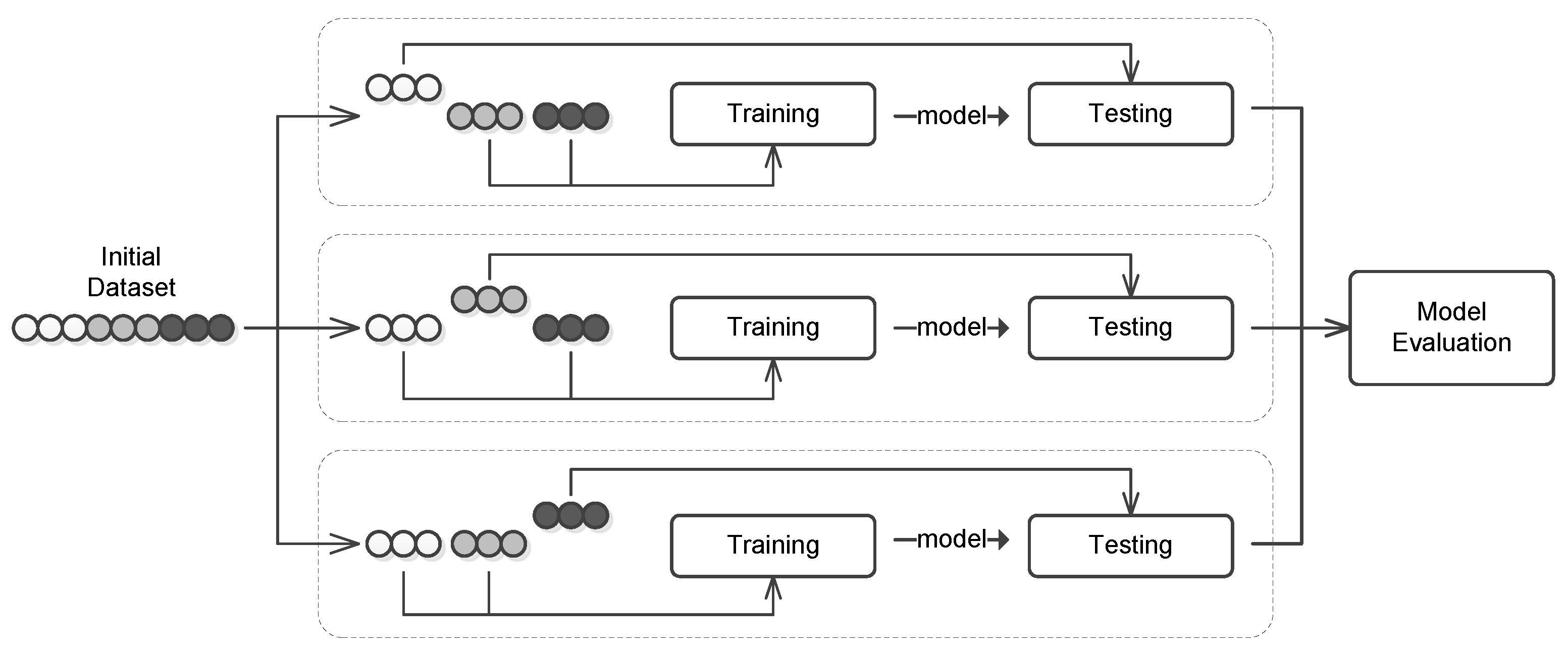
We started our analysis with the AR versions of all models. We split our sample into two parts; the sub-sample from June 2006 to September 2015 i.e., 112 months was used for training the models and the sub-sample from October 2015 to February 2018 i.e., 29 months was used to evaluate the out-of-sample forecasting accuracy on one-period-ahead forecasting.
In terms of the best AR models, our empirical findings suggest that the most accurate SVM model coupled with the linear kernel is the one that includes 11 lags of the WTI price (SVM-linear-11). The most accurate SVM model with the RBF kernel includes 5 lags of the WTI price (SVM-RBF-5) and the most accurate logistic regression AR model has 12 lags (All detailed results are available from the authors upon request).
After determining of the most accurate AR models, we augmented them with additional variables through an exhaustive search of all possible combinations. We kept the same subsamples for training and testing purposes. According to this scheme, the most accurate structural SVM-linear-11 model includes the dependent variable “Fuel oil, No. 2 NY gal”. The most accurate structural SVM-RBF-5 model includes the “Trade weighted U.S. dollar index” variable, while the most accurate structural Logit-12 model includes the variables “Fuel oil, No. 2 NY gal” and “Trade weighted U.S. dollar index”. The variable “Fuel oil, No. 2 NY gal” reports refined oil spot prices that were sold in the New York area, while the “Trade weighted U.S. dollar index” is a trade-weighted index of the U.S. dollar to a basket of foreign currencies that is based on the trading volumes of the U.S. economy with its trade partners. The directional accuracy of each model is reported in Table 2.
As we observe from Table 2, our best overall model both in in-sample and out-of-sample forecasting accuracy is the structural SVM coupled with the non-linear RBF kernel. The second most accurate model is the structural SVM model with the linear kernel, followed by the structural logistic regression model. Thus, our results corroborate with the relevant literature with respect to the forecasting superiority of the machine learning methodologies when compared to equivalent econometric methods. Moreover, we detect that certain variables are useful in forecasting oil prices as in [11], however unlike their approach, we are able to specifically identify these variables. Another finding is that all AR models are less accurate than their respective structural versions.
Interestingly, all AR or structural SVM models outperformed the RW model in terms of out-of-sample forecasting accuracy. This finding suggests that the conclusion of [6] that no model outperforms a RW may be attributed to the low forecasting ability of the econometric methodology that was applied in their study. In our dataset, the machine learning approach that we employed in this study clearly outperforms the RW model, rejecting their conclusion. Moreover, given that the AR SVM models outperform the RW model, this provides evidence against the EMH for the WTI oil market, even in its weak form. The reported directional forecasting accuracies are not common in the typical econometric literature and can be attributed to the superior forecasting ability of the machine learning approach in comparison to the probit/logit model that was used in forecasting (see [9] for more details). On several occasions, the out-of-sample forecasting accuracy was higher than the in-sample one, however this was sample dependent since the “unknown” data that was used for the out-of-sample forecasting was not used during the training phase of the models.
Our atheoretical approach has not highlighted, however, the existence of a potential causal relationship (lead-lag relationship) between interest rates and WTI oil prices, given that they were not selected through the exhaustive search step as informative variables. In order to test for the hypothesis suggested by the Hotelling’s rule that interest rates determine oil prices, we built SVM and logistic regression models using the four interest rate variables in our sample as well as the spread between the 10-year and 5-year interest rates for the U.S. with the effective federal funds rate. The use of the term spread between long and short-term rates was motivated by the need to include the expectations about future economic conditions, which are captured by the term spread. To keep things tractable, we used the same sub-samples for training and testing the forecasting accuracy and we also used the seasonal dummy variables. Unlike our atheoretical approach, we did not include lags of the dependent variable in this empirical analysis. We tested alternative lag orders of interest rates, however the models with the highest forecasting accuracy are the ones that forecast next period’s (month) oil prices based on this period’s interest rates (We also tested models that included lags of the dependent variable as regressors, which are not reported given that they exhibit lower forecasting accuracy to the models reported in Table 3. The results are available from the authors upon request.). In Table 3, we report the out-of-sample forecasting accuracy of the interest rate models.
As we observe from Table 3, all models outperform the out-of-sample accuracy of the RW model reported in Table 2 (48.28%). No model outperforms the structural RBF-SVM model of our atheoretical approach that is reported in Table 2 (67.86%), however in two cases, the forecasting accuracy reaches 64%. More specifically, the most accurate models are the SVM-RBF based on the “Effective Federal Funds Rate” and the “CBOE Interest Rate 10 Year minus Effective Federal Funds Rate”. Thus, the short-term federal funds rate seems to drive WTI oil prices and this effect is best captured by the non-linear RBF kernel, suggesting that oil market participants follow short-term interest rates closer than long-term ones.
Unlike the bulk of literature that rejects Hoteling’s rule [3], our empirical findings provide evidence in favor of interest rates driving oil prices. Although the interest rates models do not achieve the highest forecasting accuracy (and thus, they are not selected during the atheoretical step), they outperform the RW model, suggesting that they are able to forecast oil prices’ evolution. In contrast, older studies fail to do so. This discrepancy with the existing literature should be attributed to the forecasting ability of the machine learning approach, while older studies are based on OLS regressions and logistic regressions. The use of our SVM methodology with the higher forecasting accuracy in comparison to typical econometric methodologies is able to unveil the relationship between interest rates and oil prices. We leave the issue open for further research.

4. Conclusions

In this paper, we revisited the efficient market hypothesis for the oil market under a machine learning framework. In doing so, we built AR and structural forecasting models based on the Support Vector Machines methodology, spanning the period June 2006 to February 2018. Our empirical findings suggest that the AR SVM model outperforms the RW, rejecting even the weak form of efficiency in the oil market. Through an exhaustive search among a pool of 38 potential regressors, we found that when we couple the AR SVM model with the trade-weighted index of U.S. dollars to a basket of foreign currencies, we manage to increase the out-of-sample forecasting accuracy to 67.8%. Moreover, when we focus explicitly on the relationship between oil prices and interest rates, our machine learning approach is able to unveil the existence of a causal relationship, unlike previous studies that use typical econometric methods. This finding is an indication in support of Hotelling’s rule, however we leave this issue for future research.

Author Contributions

T.P. and P.G. contributed on the conceptualization, methodology organization, evaluation of the models and the results and the revision of the paper, A.D. on obtaining and processing the data, performing all the models selection and experiments with respect to the empirical part, and provided the initial draft of the paper, while V.P. worked on the organization, evaluation of the results, initial and further writing and the final revision of the paper.

Funding

This research received no external funding.

Conflicts of Interest

The authors declare no conflict of interest.

References

  1. Hotelling, H. The economics of exhaustible resources. J. Political Econ. 1931, 39, 137–175. [Google Scholar] [CrossRef]
  2. Solow, R. On the Intergenerational Allocation of Natural Resources. Scand. J. Econ. 1986, 88, 141–149. [Google Scholar] [CrossRef]
  3. Gaudet, G. Natural Resource Economics under the Rule of Hotelling. Can. J. Econ. 2007, 40, 1033–1059. [Google Scholar] [CrossRef]
  4. Hamilton, J.D. Oil and the Macroeconomy Since World War II. J. Political Econ. 1983, 91, 228–248. [Google Scholar] [CrossRef]
  5. Baumeister, C.; Killian, L. What Central Bankers need to Know about forecasting oil prices. Int. Econ. Rev. 2014, 55, 869–889. [Google Scholar] [CrossRef]
  6. Baumeister, C.; Killian, L. Forty Years of Oil Price Fluctuations: Why the Price of Oil May Still Surprise Us. J. Econ. Perspect. 2016, 30, 139–160. [Google Scholar] [CrossRef]
  7. Knetsch, T.A. Forecasting the price of crude oil via convenience yield predictions. J. Forecast. 2007, 26, 527–549. [Google Scholar] [CrossRef] [Green Version]
  8. Alquist, R.; Kilian, L. What do we learn from the price of crude oil futures. J. Appl. Econom. 2010, 25, 539–573. [Google Scholar] [CrossRef]
  9. Alquist, R.; Kilian, L.; Vigfusson, R.J. Forecasting the Price of Oil, Handbook of Economic Studies; Elsevier: Amsterdam, The Netherlands, 2013. [Google Scholar]
  10. Wang, J.; Athanasopoulos, G.; Hyndman, R.; Wang, S. Crude oil price forecasting based on internet concern using an extreme learning machine. Int. J. Forecast. 2018, 34, 665–677. [Google Scholar] [CrossRef]
  11. Zhao, Y.; Li, J.; Yu, L. A deep learning ensemble approach for crude oil price forecasting. Energy Econ. 2017, 66, 9–16. [Google Scholar] [CrossRef]
  12. Yu, L.; Wang, S.; Lai, K.K. Forecasting crude oil price with an EMD-based neural network ensemble learning paradigm. Energy Econ. 2008, 30, 2623–2635. [Google Scholar] [CrossRef]
  13. Yu, L.; Zhao, Y.; Tang, L. A compressed sensing based AI learning paradigm for crude oil price forecasting. Energy Econ. 2014, 46, 236–245. [Google Scholar] [CrossRef]
  14. Shin, H.; Hou, T.; Park, K.; Park, C.-K.; Choi, S. Prediction of movement direction in crude oil prices based on semi-supervised learning. Decis. Support Syst. 2013, 55, 348–358. [Google Scholar] [CrossRef]
  15. Plakandaras, V.; Gupta, R.; Gogas, P.; Papadimitriou, T. Forecasting the U.S, Real House Price Index. Econ. Model. 2015, 45, 259–267. [Google Scholar] [CrossRef]
  16. Khandani, A.E.; Kim, A.J.; Lo, A.W. Consumer credit-risk models via machine-learning algorithms. J. Bank. Financ. 2010, 34, 2767–2787. [Google Scholar] [CrossRef] [Green Version]
  17. Cortes, C.; Vapnik, V. Support-Vector Networks. Mach. Learn. 1995, 20, 273–297. [Google Scholar] [CrossRef]
  18. Chang, C.; Lin, C. LIBSVM: A library for support vector machines. ACM Trans. Intell. Syst. Technol. 2011, 27, 1–27. [Google Scholar] [CrossRef]
  19. Tay, F.; Cao, L. Modified support vector machines in financial time series forecasting. Neurocomputing 2002, 48, 847–861. [Google Scholar] [CrossRef]
  20. Fama, E. The Behavior of Stock Market Prices. J. Bus. 1965, 38, 34–105. [Google Scholar] [CrossRef]
Figure 1. Hyperplane selection and support vectors. The two classes are represented with circles and triangles. The SVs (Support Vectors) are indicated by the pronounced hollow (red) circles and triangles, the margin lines are represented with the continuous lines and the hyperplane (linear classifier) is represented with the dotted line.
Forecasting 01 00011 g001
Figure 2. The data space: The non-separable two-class scenario (left) and the separable case in the feature space after the projection (right).
Forecasting 01 00011 g002
Figure 3. An example of an SVM (Support Vector Machine) classification using the RBF (Radial Basis Function) kernel. The two classes are separated with a linear separator on a higher dimensional space, which when re-projected back into its original dimensions becomes a non-linear function. The circled instances are the Support Vectors defining the decision boundary, and the instances with a diamond rounding are misclassified instances.
Forecasting 01 00011 g003
Figure 4. Overview of a 3-fold Cross Validation training scheme. It shows that each subset is used as a testing sample, while the others are used for training the model for each parameters’ value combination.
Forecasting 01 00011 g004
Figure 5. A three-step coarse to fine grid search procedure for two parameters ×1 and ×2, where the forecasting accuracy of the model rises as one moves from coarse to dense (darker) areas of the grid.
Forecasting 01 00011 g005
Table 1. Descriptive Statistics.
NoNameMeanStandard DeviationSkewnessKurtosis
Panel A: Stock Indices
1Mexico IPC Index10.490.26−0.822.85
2NASDAQ Index8.090.400.182.05
3S&P5007.340.30−0.062.30
Panel B: Exchange Rates
4EUR/USD exchange rate0.250.10−0.312.31
5Trade weighted U.S. dollar index4.430.090.482.13
Panel C: Commodities
6Silver prices2.930.340.692.87
7Gold prices7.040.28−0.682.77
Panel D: Interest Rates
8CBOE Interest Rate 10 Year2.840.960.982.46
9Effective Federal Funds Rate1.031.711.784.58
10Fed 5-Year Treasury Constant Maturity Rate2.061.141.193.60
113-Month London Interbank Offered Rate (LIBOR)1.371.731.563.91
Panel E: Oil product prices
12Fuel oil, No. 2 NY gal0.750.32−0.266.74
13Brent oil prices 4.330.36−0.291.40
14Conventional Gasoline Prices: New York Harbor0.740.29−0.322.30
15Conventional Gasoline Prices: U.S. Gulf Coast0.710.29−0.342.23
16Reformulated Gasoline RBOB0.810.27−0.372.26
17No. 2 Heating Oil Prices: New York Harbor0.750.32−0.262.06
18Ultra-Low-Sulfur No. 2 Diesel Prices: U.S. Gulf Coast0.770.32−0.302.10
19Ultra-Low-Sulfur No. 2 Diesel Prices: New York Harbor0.790.31−0.292.09
20Ultra-Low-Sulfur No. 2 Diesel Fuel Prices: Los Angeles0.800.30−0.312.17
21Propane Prices: Mont Belvieu, Texas−0.080.40−0.542.46
22Henry Hub Natural Gas Spot Price1.380.410.573.03
Panel F: Future contracts
23Natural Gas Futures Contract 11.410.410.622.90
24Natural Gas Futures Contract 21.430.410.412.76
25Natural Gas Futures Contract 31.460.420.642.70
26Natural Gas Futures Contract 41.480.420.662.68
27Cushing OK Crude Oil Future Contract 14.280.32−0.362.08
28Cushing OK Crude Oil Future Contract 24.290.31−0.332.05
29Cushing OK Crude Oil Future Contract 34.300.31−0.322.03
30Cushing OK Crude Oil Future Contract 44.300.30−0.312.03
31New York Harbor RBOB Gasoline Future Contract 10.750.30−0.302.12
32New York Harbor RBOB Gasoline Future Contract 20.750.29−0.221.97
33New York Harbor RBOB Gasoline Future Contract 30.750.28−0.181.91
34New York Harbor RBOB Gasoline Future Contract 40.740.27−0.151.84
35New York Harbor No. 2 Heating Oil Future Contract 10.770.31−0.211.98
36New York Harbor No. 2 Heating Oil Future Contract 20.780.30−0.211.99
37New York Harbor No. 2 Heating Oil Future Contract 30.780.30−0.202.00
38New York Harbor No. 2 Heating Oil Future Contract 40.790.29−0.192.01
Table 2. Directional Forecasting Accuracy.
ModelKernelAR (autoregressive) LagsIn-Sample AccuracyOut-Of-Sample Accuracy
RW (Random Walk)-042.8648.28
AR SVM modelLinear1160.7162.38
Structural SVM modelLinear1167.3364.29
AR SVM modelRBF564.2954.96
Structural SVM modelRBF569.3767.86
AR Logistic Regression model-1252.0037.93
Structural Logistic Regression model-1259.4664.29
Note: All accuracy values are percentages.
Table 3. Out-of-sample Directional Forecasting Accuracy of the interest rate models.
Input VariablesLogistic RegressionSVM- Linear KernelSVM- RBF Kernel
CBOE Interest Rate 10 Year35.715035.71
Effective Federal Funds Rate54.0557.1564.29
Fed 5-Year Treasury Constant Maturity Rate35.715060.71
3-Month London Interbank Offered Rate (LIBOR)54.055060.71
CBOE Interest Rate 10 Year minus Effective Federal Funds Rate53.575064.29
Fed 5-Year Treasury Constant Maturity Rate minus Effective Federal Funds Rate54.0553.5757.14
Note: All values are percentages.

