A Two-Stage Changepoint–Copula Framework for Non-Stationary Count Time Series: Application to Tropical Cyclones

Abstract

Cross-basin tropical cyclone variability may exhibit complex, non-linear dependence structures influenced by large-scale climate modes and potential regime shifts. Reliance on traditional linear correlation measures without accounting for structural changes can therefore lead to misleading interpretations of global storm relationships. This study investigates the regional dependence structures of tropical cyclone counts across six major ocean basins (NA, ENP, WNP, NI, SI, and SP) from 1980 to 2024. We adopt a two-stage analytical framework integrating changepoint detection and copula modeling to address non-stationarity in both marginal distributions and dependence structures. First, we identify a significant structural break in the year 2000 via a penalised likelihood applied jointly to the $d=6$-variate Poisson series, with inter-basin dependence captured by a latent Gaussian process (the construction used by Lund et al. (2025). This is mathematically equivalent to a Gaussian copula with Poisson margins (Genest and Nešlehová (2007)). Then, we apply bivariate copula models separately to the pre- and post-2000 regimes using the randomized probability integral transform with results averaged over 500 replications of the auxiliary uniforms to mitigate randomization noise. The results reveal substantial non-stationarity, most notably a 59% increase in North Atlantic storm frequency and a fundamental reorganization of global dependence structures, while dependence structures evolved from primarily symmetric and weak (dominated by Gaussian and Clayton copulas) to more complex and stronger dependencies (increased Frank and Gumbel copulas). Notably, a statistically significant ($p<0.001$) and strong negative dependence emerged between the Southern Pacific and Northern Indian basins ($\tau =-0.464$) in the recent regime. The inclusion of changepoint detection significantly improves model fit and reveals a fundamental reorganization of global tropical cyclone teleconnections, with enhanced coordination between basins in the contemporary climate regime. Modeling these regimes separately, as opposed to a single stationary period, uncovers a shift towards more complex, tail-dependent copula families (Gumbel, Clayton) in the recent era. These findings have important implications for climate risk assessment, seasonal forecasting, and understanding the impacts of climate change on global storm patterns. The proportion of Gumbel copulas (capturing upper-tail dependence) increased from 7% to 20%, while Gaussian copulas decreased from 53% to 33%, indicating more complex, extreme-value-focused dependencies in the contemporary climate. Due to small sample sizes ($n_1=20$, $n_2=25$), copula and dependence estimates are exploratory, not confirmatory. Interpretations reflect this power constraint, utilizing Benjamini–Hochberg adjustments for significance.

1. Introduction

Tropical cyclones (TC) are among the most destructive natural hazards, causing significant socioeconomic impacts globally. Understanding the regional dependence structures between different ocean basins is crucial for improving seasonal forecasts, assessing aggregate climate risks, and identifying potential teleconnection patterns influenced by large-scale climate modes. Traditional correlation measures (e.g., Pearson’s $\rho$) are inadequate for capturing complex, non-linear dependence structures and are not invariant under monotonic transformations. In 2022, Chand et al. [1] reported declining global and regional tropical cyclone frequency during the twentieth century. Moreover, if there are any significant changes or shifts in the storm counts over the years, then only considering traditional correlation measures (e.g., Pearson’s $\rho$) without considering the structural shift might give a misleading interpretation. While machine learning has been extensively benchmarked across a wide range of fields (e.g., clinical risk prediction and social aspects [2,3,4,5,6,7]), the non-stationary, multivariate nature data (e.g., climate extremes) demands a different analytical approach that captures evolving dependence structures [8,9,10]. Our study addresses this need by integrating changepoint detection with copula modeling.

Copula theory, introduced by Sklar [11], provides a versatile framework for multivariate modeling by decoupling marginal distributions from their underlying dependence structure. For a comprehensive overview of copula families and their properties, see [12]. This approach has been successfully applied in various fields including finance, hydrology, and climate science. For a comprehensive review of dependence modeling in the environmental sciences, see [13]. However, the application to TC counts presents unique challenges: (1) count data are discrete rather than continuous, requiring appropriate transformations; (2) both marginal distributions and dependence structures may exhibit non-stationarity over time due to climate shift and natural variability. The work of [14] provides the theoretical foundation for applying copula functions to count data while maintaining statistical rigor. The challenge of non-stationarity in climate extremes is a growing field of study [15]. Ref. [16] identified a significant shift in Atlantic hurricane activity beginning in 1995, noting a doubling of overall basin activity and a 2.5-fold increase in major hurricanes compared to the 1971–1994 quiet period. This shift suggests that the era spanning the turn of the 21st century represents a distinct high-activity regime driven by multidecadal climate modes. Detecting and attributing such shifts is critical, as the concept of a stationary climate baseline becomes increasingly obsolete [17].

For instance, ref. [18] demonstrated that anthropogenic global warming accounted for nearly half of the anomalous sea surface warming in the North Atlantic (NA) during the record 2005 hurricane season, suggesting that climate shift has fundamentally altered the environmental baseline for tropical cyclone activity beyond natural multidecadal cycles and historical norms.

Furthermore, climate modeling experiments indicate that seasonal basin-wide TC frequency is not limited by the presence of specific synoptic-scale disturbances. Suppression of African easterly waves in regional climate simulations produces no statistically significant change in seasonal Atlantic TC counts [19], suggesting that large-scale environmental conditions, rather than localized seeding mechanisms, regulate climatological TC frequency. Since such large-scale controls may influence multiple basins simultaneously and may shift across climatic regimes, modeling the evolving cross-basin dependence structure becomes essential.

This study addresses these challenges through a two-stage analytical framework that first identifies structural breaks and then applies copula models within homogeneous regimes. In this two-stage analytical framework, changepoint detection with copula modeling was integrated. We first identify significant structural breaks in the annual storm count series for each basin, then apply bivariate copula models separately within each homogeneous regime. This approach allows us to examine how regional dependence structures have evolved in response to documented shifts in global climate patterns around the structural breakpoints. Based on the penalized likelihood method described in Section 2.5 ((with the Bayesian Information Criterion (BIC)), we identified a single dominant changepoint at 2000, which aligns with documented climate regime shifts [16,18] and divides our 45-year record into two climatically distinct periods: 1980–1999 and 2000–2024. This alignment is reported as ex post consistency, not as an a priori constraint on the search: the year 2000 is the data-driven minimizer of the BIC objective over the admissible class of multivariate changepoint configurations (Section 2.6), and we report sensitivity to nearby break years in Section 4.3. This two-regime approach is validated by the substantial changes in marginal distributions: the North Atlantic exhibits a 59% increase in mean storm count (from 10.43 to 16.58), while the Southern Pacific shows a 22% decrease (from 11.81 to 9.21). Such dramatic shifts in basin-level activity would violate the stationarity assumption required for traditional single-period analysis. Ref. [20] shows increasing frequency of extreme Indian Ocean Dipole (IOD) events from the twentieth to the twenty-first century.

The primary objective of this study is to develop and apply a two-stage analytical framework that integrates joint multivariate changepoint detection with regime-specific copula modeling for non-stationary count time series, and to use this framework to characterize how tropical cyclone (TC) teleconnections across six ocean basins have evolved between 1980 and 2024. Existing works that combine changepoint detection with dependence modeling typically (i) treat each series separately at the detection step, (ii) work with continuous variables, or (iii) restrict the copula to a single family. Our framework departs from all three: it uses a joint d-variate detector (Lund et al., 2025 [21]) over discrete Poisson margins, applies the randomized probability integral transform (PIT) with $B_{\mathrm{MC}}$ Monte-Carlo averaging, and selects pair- and regime-specific copula families from four candidates. The combination of joint multivariate detection on discrete data plus pair-specific regime copulas is, to our knowledge, new in the tropical-cyclone literature.

The paper is organized as follows. In Section 2, the theory of Copula, structural break, and the two-stage framework of Copula-Change points were presented. Section 3 includes the simulation study for the two-stage framework. Section 4 contains the real data findings and the analysis results. Section 5 includes the discussion, and finally, the conclusion of the research work in Section 6.

2. Theoretical Framework and Methodology

To formally characterize cross-basin dependence under potential regime shifts, we adopt a copula-based modeling framework that enables flexible separation of marginal behavior from dependence structure. This framework is particularly suitable for tropical cyclone count data, where marginal distributions may differ across basins and evolve over time, while dependence patterns may exhibit non-linear and asymmetric characteristics. The following section outlines the theoretical foundations of copula modeling and the parametric families used in this study.

For clarity of indices, we collect the notation used throughout the paper in

Table 1. Notation used throughout the paper.

Symbol	Meaning
N	Length of each time series ($N=45$ years for the cyclone data)
d	Number of series (basins); $d=6$ for the cyclone data, $d=2$&3 in the simulation
b	Series, $b=1,\dots ,d$
t	Time (year), $t=1,\dots ,N$
$X_b^t$	Annual count for series b at time t ($X_{br}^t$ for regime r)
m	Number of changepoints
${\nu }_r$	r-th changepoint location, ${\nu }_0=0,{\nu }_{m+1}=N$
$\mathit{\eta }$	Changepoint configuration ${(m;{\nu }_1,\dots ,{\nu }_m)}^{\prime }$
r	Regime, $r=1,\dots ,m+1$
$n_r$	Length of regime r, $n_r={\nu }_r-{\nu }_{r-1}$
${\mu }_{br}$	Poisson rate of series b in regime r
$\mathbf{R}$	$d\times d$ Gaussian-copula correlation matrix
${\mathbf{R}}_{\tau }^{\left(r\right)}$	$d\times d$ Kendall’s tau matrix in regime r
$U_{br}^t$	PIT-transformed value of $X_b^t$ in regime r
$V_{br}^t$	Auxiliary $\mathrm{Uniform}(0,1)$ used in the randomized PIT
$B_{\mathrm{MC}}$	Number of Monte Carlo replications (over $V_{br}^t$ for the PIT, or over data for simulations)
${\theta }_C$	Generic copula parameter; $\tau$ denotes the corresponding Kendall’s tau
$\mathcal{l}(·)$	Log-likelihood
$O\left(\mathit{\eta }\right)$	Penalized objective: $-2ln{L}_{\mathrm{opt}}\left(\mathit{\eta }\right)+P\left(\mathit{\eta }\right)$

. We use ${\nu }_1<\dots <{\nu }_m$ exclusively for changepoint times, $\tau$ exclusively for Kendall’s tau, b for the series ($b=1,\dots ,d$), r for the regime ($r=1,\dots ,m+1$), and t for the time ($t=1,\dots ,N$).

2.1. The Probability Integral Transform (PIT)

A fundamental step in applying copula theory to continuous variables is the transformation of marginal data to a uniform scale using the Probability Integral Transform (PIT).

Theorem 1

(Probability Integral Transform for Continuous Variables). Let X be a continuous random variable with cumulative distribution function $F_X\left(x\right)$. Then, the random variable $U=F_X\left(X\right)$ follows a standard uniform distribution, i.e., $U\sim U(0,1)$.

This is a standard result; we omit the proof and refer the reader to [22], Theorem 2.1.10.

Probability Integral Transform for Discrete Data: A fundamental requirement for applying standard copula theory is that the input data must be continuous and uniformly distributed on $[0,1]$. Applying copulas directly to discrete count data can lead to biased dependence estimates. For the discrete case (e.g., storm counts on $\{0,1,2,\dots \}$), we apply the randomized probability integral transform [14,23] defined as:

$$U=F_X\left(X^{-}\right)+V·[F_X\left(X\right)-F_X\left(X^{-}\right)],\mathrm{if}X\in \{0,1,2,3,\dots \},$$

(1)

where $F_X\left(x^{-}\right)=P(X<x)$ is the left-hand limit of the CDF at x, and V is a random variable independent of X, uniformly distributed on $[0,1]$. This transformation ensures that U follows a standard uniform distribution.

Caveats and reproducibility under the randomized PIT. For discrete margins, the underlying copula is not unique, so any copula-based dependence summary depends on the auxiliary uniforms V. To mitigate the resulting randomization noise which is non-negligible at the regime-specific sample sizes (used here $n_r=20$ and 25 for TC data), the copula-based quantity reported in Section 4.2 and Section 4.3 is averaged over $B_{\mathrm{MC}}=500$ to independent realizations of $\left\{V_{br}^t\right\}$ with seed fixed for reproducibility (results of $B_{MC}=500$ are available at

Table A1. Copula results for the entire analysis period. Note: ${\tau }_C$ and $p_C$ refer to copula Kendall’s tau and its p-value; SDs are given for the estimated parameter and ${\tau }_C$; $T_C$ BH FDR is the Benjamini–Hochberg false discovery rate adjusted p-value for ${\tau }_C$; LL is log-likelihood; $p_{\mathrm{GOF}}$ is the GOF p-value. Significant p-values (<0.05) are in bold.

Basin 1	Basin 2	Copula	E. Par.	E. Par.-SD	${\mathit{\tau }}_{\mathit{C}}$	${\mathit{\tau }}_{\mathit{C}}$-SD	${\mathit{p}}_{\mathit{C}}$	${\mathit{T}}_{\mathit{C}}$ BH FDR	LL	${\mathit{p}}_{\mathbf{GOF}}$
E. North Pacific	North Atlantic	Gaussian	−0.461	0.549	−0.176	0.015	0.006	0.081	3.542	0.579
E. North Pacific	Northern Indian	Gumbel	1.125	0.016	0.111	0.013	0.209	0.330	1.329	0.760
E. North Pacific	Southern Indian	Frank	0.985	0.099	0.108	0.011	0.272	0.340	0.601	0.322
E. North Pacific	Southern Pacific	Gumbel	1.100	0.011	0.091	0.009	0.242	0.330	0.814	0.750
E. North Pacific	W. North Pacific	Clayton	0.292	0.018	0.127	0.007	0.067	0.186	2.045	0.909
North Atlantic	Northern Indian	Frank	0.626	0.151	0.069	0.017	0.469	0.502	0.281	0.783
North Atlantic	Southern Indian	Frank	−0.567	0.118	−0.063	0.014	0.469	0.502	1.264	0.671
North Atlantic	Southern Pacific	Frank	−1.867	0.100	−0.201	0.010	0.016	0.082	2.667	0.389
North Atlantic	W. North Pacific	Gaussian	−0.361	0.430	−0.123	0.014	0.087	0.186	1.417	0.307
Northern Indian	Southern Indian	Gaussian	−0.330	0.036	−0.214	0.024	0.079	0.186	1.158	0.529
Northern Indian	Southern Pacific	Gumbel	1.113	0.107	0.107	0.018	0.236	0.330	0.848	0.110
Northern Indian	W. North Pacific	Frank	−2.326	0.310	−0.245	0.030	0.063	0.186	1.311	0.141
Southern Indian	Southern Pacific	Frank	0.574	0.116	0.064	0.013	0.545	0.545	0.192	0.431
Southern Indian	W. North Pacific	Gaussian	0.611	0.627	0.248	0.012	0.011	0.081	2.361	0.679
Southern Pacific	W. North Pacific	Frank	−1.405	0.234	−0.156	0.014	0.167	0.313	0.894	0.294

Note: All estimates are based on 500 ($B_{MC}=500$) replicates. GOF p-values $>0.05$ indicate an acceptable fit.

and

Table A2. Comparison of copula results across two regimes (1980–1999 and 2000–2024). Note: ${\tau }_C$ and $p_C$ refer to copula Kendall’s tau and its p-value; SDs are given for the estimated parameter and ${\tau }_C$; $T_C$ BH FDR is the Benjamini–Hochberg false discovery rate adjusted p-value for ${\tau }_C$; LL is log-likelihood; $p_{\mathrm{GOF}}$ is the GOF p-value. Significant p-values (<0.05) are in bold.

Basin 1	Basin 2	Copula	E. Par.	E. Par.-SD	${\mathit{\tau }}_{\mathit{C}}$	${\mathit{\tau }}_{\mathit{C}}$-SD	${\mathit{p}}_{\mathit{C}}$	${\mathit{T}}_{\mathit{C}}$ BH FDR	LL	${\mathit{p}}_{\mathbf{GOF}}$
Regime 1: 1980–1999
E. North Pacific	North Atlantic	Gaussian	−0.433	0.018	−0.285	0.013	0.004	0.061	3.252	0.799
E. North Pacific	Northern Indian	Gumbel	1.152	0.017	0.132	0.013	0.201	0.378	1.526	0.349
E. North Pacific	Southern Indian	Frank	1.188	0.102	0.130	0.011	0.282	0.389	0.579	0.620
E. North Pacific	Southern Pacific	Gaussian	0.886	0.614	0.156	0.015	0.146	0.364	1.017	0.680
E. North Pacific	W. North Pacific	Clayton	0.061	0.033	0.029	0.011	0.770	0.771	0.050	0.786
North Atlantic	Northern Indian	Gaussian	−0.030	0.116	−0.035	0.034	0.739	0.771	0.066	0.613
North Atlantic	Southern Indian	Clayton	0.314	0.037	0.136	0.014	0.202	0.378	0.894	0.924
North Atlantic	Southern Pacific	Frank	−1.076	0.332	−0.128	0.014	0.285	0.389	0.564	0.920
North Atlantic	W. North Pacific	Frank	−0.272	0.230	−0.029	0.033	0.771	0.771	0.046	0.728
Northern Indian	Southern Indian	Gaussian	−0.410	0.383	−0.198	0.025	0.143	0.364	0.944	0.732
Northern Indian	Southern Pacific	Gaussian	0.731	0.459	0.183	0.022	0.105	0.364	1.289	0.418
Northern Indian	W. North Pacific	Frank	−1.826	0.339	−0.196	0.033	0.273	0.389	0.530	0.394
Southern Indian	Southern Pacific	Frank	−0.294	0.206	−0.049	0.015	0.665	0.771	0.099	0.705
Southern Indian	W. North Pacific	Gaussian	0.478	0.039	0.311	0.019	0.012	0.086	1.998	0.855
Southern Pacific	W. North Pacific	Gaussian	−0.397	0.019	−0.260	0.013	0.024	0.119	1.982	0.213
Regime 2: 2000–2024
E. North Pacific	North Atlantic	Frank	−2.514	0.151	−0.263	0.014	0.022	0.083	2.147	0.468
E. North Pacific	Northern Indian	Frank	0.567	0.549	0.038	0.075	0.743	0.743	0.065	0.651
E. North Pacific	Southern Indian	Frank	0.426	0.299	0.060	0.023	0.706	0.743	0.077	0.453
E. North Pacific	Southern Pacific	Gaussian	−0.500	0.466	−0.132	0.032	0.480	0.743	0.232	0.258
E. North Pacific	W. North Pacific	Clayton	0.613	0.039	0.234	0.012	0.018	0.083	2.902	0.728
North Atlantic	Northern Indian	Gaussian	0.278	0.410	0.067	0.036	0.656	0.743	0.115	0.289
North Atlantic	Southern Indian	Gaussian	0.095	0.020	0.061	0.013	0.631	0.743	0.119	0.625
North Atlantic	Southern Pacific	Gaussian	0.127	0.184	0.054	0.020	0.693	0.743	0.085	0.315
North Atlantic	W. North Pacific	Frank	−1.356	0.129	−0.148	0.014	0.261	0.489	0.605	0.104
Northern Indian	Southern Indian	Gumbel	1.543	0.254	0.365	0.069	0.017	0.083	1.399	0.533
Northern Indian	Southern Pacific	Gaussian	−0.829	0.777	−0.493	0.031	<0.001	<0.001	2.683	0.762
Northern Indian	W. North Pacific	Gaussian	−0.597	1.549	−0.115	0.208	0.256	0.489	0.390	0.450
Southern Indian	Southern Pacific	Gumbel	1.435	0.159	0.304	0.055	0.070	0.209	0.887	0.527
Southern Indian	W. North Pacific	Gumbel	1.028	0.303	0.114	0.027	0.571	0.743	0.141	0.224
Southern Pacific	W. North Pacific	Frank	−2.759	0.355	−0.285	0.032	0.091	0.227	0.919	0.826

Note: All estimates are based on 500 (B_MC = 500) replicates. GOF p-values > 0.05 indicate an acceptable fit.

). We also acknowledge that principled alternatives developed specifically for discrete margins—the discrete copula framework of [24], the rectangular-support inference of [25], and the empirical discrete copula process of [26] avoid the randomization step at the cost of less mature software and finite-sample theory; we identify these as the natural next direction in Section 5 (Limitations and Future Work).

2.2. Copula Theory

A copula is a multivariate distribution function with uniform margins on $[0,1]$. According to Sklar’s Theorem [11], any joint distribution function H of random variables $(X_1,X_2)$ with marginal CDFs $F_1$ and $F_2$ can be expressed as:

$$H(x_1,x_2)=C(F_1\left(x_1\right),F_2\left(x_2\right)).$$

(2)

where C is a copula. If $F_1$ and $F_2$ are continuous, C is unique. The joint probability density function can be factorized as:

$$h(x_1,x_2)=c(F_1\left(x_1\right),F_2\left(x_2\right))·f_1\left(x_1\right)·f_2\left(x_2\right).$$

(3)

where c is the copula density, and $f_1$, $f_2$ are the marginal densities.

If $F_1$ and $F_2$ are continuous and C is a copula, then H is a joint CDF with margins $F_1$ and $F_2$, and the corresponding joint density factorization as

$$h(x_1,x_2)={\displaystyle \frac{{\mathsf{\partial }}^{2}H(x_1,x_2)}{\mathsf{\partial }{x}_1\mathsf{\partial }{x}_2}}=c\left(F_1\left(x_1\right),F_2\left(x_2\right)\right)·f_1\left(x_1\right)·f_2\left(x_2\right),c(u_1,u_2)={\displaystyle \frac{{\mathsf{\partial }}^{2}C(u_1,u_2)}{\mathsf{\partial }{u}_1\mathsf{\partial }{u}_2}},$$

(4)

where $f_1,f_2$ are the marginal densities and c is the copula density. This single factorization, which subsumes the two duplicated displays in the previous version, is what enables separate modeling of the marginals $(f_1,f_2)$ and the dependence $\left(c\right)$.

2.3. Common Choices of Parametric Copula Families

Common choices of copula include three one-parameter Archimedean copula families (Clayton, Gumbel, Frank) together with the (non-Archimedean elliptical) Gaussian copula, each capturing different dependence characteristics (Kendall’s tau ($\tau$) is the measure of dependence).

Table 2. Characteristics and application of parametric copula families.

Family	Param. Range	Sym.	Tail	Summary and Application
Gaussian	$\theta \in [-1,1]$	Yes	None	Appropriate when dependence is symmetric and tail behavior is light; useful as a baseline.
Clayton	$\theta \in [0,\infty )$	No	Lower	Emphasis on lower tail dependence; ideal for modeling “crashes” or joint low-activity periods (e.g., losses).
Gumbel	$\theta \in [1,\infty )$	No	Upper	Emphasis on upper tail dependence; ideal for modeling joint “peaks” or high-activity years (e.g., floods).
Frank	$\theta \in \mathbb{R}\setminus \left\{0\right\}$	Yes	None	Strongest dependence at the center; versatile for modeling both +ve and −ve dependence structures.

shows some properties of select copula families. The present study uses these four one-parameter families on a pair-by-pair basis. For genuinely multivariate dependence in $d\ge 3$ series with heterogeneous pairwise dependencies, the standard route is a vine (C-vine, D-vine, or regular vine) copula construction [27,28,29]; in the simulation study (Section 3), we use a single exchangeable parametric $d=3$ copula in which all pairwise ${\tau }_{ij}^{\left(r\right)}$ are equal within a regime, so no compatibility issue arises. Vine-copula extension of the framework is identified as future work (Section 5).

1.

Gaussian copula: Symmetric dependence with no tail dependence

$$C_{Ga}(u_1,u_2;\theta )={\mathsf{\Phi }}_{\theta }({\mathsf{\Phi }}^{-1}\left(u_1\right),{\mathsf{\Phi }}^{-1}\left(u_2\right));\theta \in [-1,1];\tau ={\displaystyle \frac{2}{\pi }}arcsin\left(\theta \right).$$

(5)

2.

Clayton copula: Lower tail dependence, asymmetric

$$C_{Cl}(u_1,u_2;\theta )={\left(max\left\{u_1^{-\theta }+u_2^{-\theta }-1;0\right\}\right)}^{-1/\theta };\theta \ge 0;\tau ={\displaystyle \frac{\theta }{\theta +2}}.$$

(6)

3.

Gumbel copula: Upper tail dependence, asymmetric

$$C_{Gu}(u_1,u_2;\theta )=exp\left(-{\left[{(-ln{u}_1)}^{\theta }+{(-ln{u}_2)}^{\theta }\right]}^{1/\theta }\right);\theta \ge 1;\tau =1-{\displaystyle \frac{1}{\theta }}.$$

(7)

4.

Frank copula: Symmetric dependence, no tail dependence

$$C_{Fr}(u_1,u_2;\theta )=-{\displaystyle \frac{1}{\theta }}ln\left(1+{\displaystyle \frac{(e^{-\theta u_1}-1)(e^{-\theta u_2}-1)}{e^{-\theta }-1}}\right);\theta \in \mathbb{R}\setminus \left\{0\right\};\tau =1-{\displaystyle \frac{4}{\theta }}[1-D_1\left(\theta \right)].$$

(8)

2.4. Measures of Dependence

While Pearson’s correlation ($\rho$) is the standard measure of linear association, it is inadequate for this study for three reasons. First, Pearson’s correlation assumes a linear relationship and bivariate normality, whereas counts (tropical cyclone teleconnections) could be non-linear and governed by asymmetric tail dependencies. Second, Pearson’s $\rho$ is not invariant under monotonic transformations; in contrast, Kendall’s tau ($\tau$) is a rank-based measure that remains consistent regardless of the marginal distribution’s shape. Third, since counts (tropical cyclone) are discrete, Kendall’s $\tau$ provides a more reliable foundation for the Probability Integral Transform (PIT), allowing for a mathematically consistent bridge between the discrete count space and the continuous copula space. Kendall’s rank correlation coefficient $\tau$ provides a non-parametric, copula-based measure of dependence. For a copula C, Kendall’s $\tau$ can be expressed as [30]:

$$\tau =4\int {\int }_{{[0,1]}^2}C(u_1,u_2)dC(u_1,u_2)-1.$$

(9)

This leads to specific relationships between $\tau$ and the copula parameter $\theta$ for each family.

Gaussian: $\tau ={\displaystyle \frac{2}{\pi }}arcsin\left(\theta \right)$,	Clayton: $\tau ={\displaystyle \frac{\theta }{\theta +2}}$,
Gumbel: $\tau =1-{\displaystyle \frac{1}{\theta }}$,	Frank: $\tau =1-{\displaystyle \frac{4}{\theta }}[1-D_1\left(\theta \right)]$,

where $D_1\left(\theta \right)$ is the Debye function of order 1.

The Frank copula parameter $\theta$ is related to Kendall’s $\tau$ through the Debye function. This function is necessary because the integral involved in the expectation of the Frank copula does not reduce to elementary algebraic terms. The Debye function of order n, denoted $D_n\left(x\right)$, is defined by the integral:

$$D_n\left(x\right)={\displaystyle \frac{n}{x^n}}{\int }_0^x{\displaystyle \frac{t^n}{e^t-1}}dt$$

where n is a positive integer, x is a real argument, and the function is used primarily in the Debye model for the specific heat capacity of solids. For the specific case where the order is $n=1$, the function simplifies to the first-order Debye integral:

$$D_1\left(x\right)={\displaystyle \frac{1}{x}}{\int }_0^x{\displaystyle \frac{t}{e^t-1}}dt$$

To provide a compact summary of all pairwise dependencies, we define the symmetric Kendall’s tau matrix $R_{\tau }$. For a d-dimensional system (e.g., d ocean basins), this matrix is given by,

$${\mathbf{R}}_{\tau }={\left({\tau }_{ij}\right)}_{i,j=1,\dots ,d}=\left(\begin{array}{ccccc}1& {\tau }_{12}& {\tau }_{13}& \dots & {\tau }_{1d}\\ {\tau }_{21}& 1& {\tau }_{23}& \dots & {\tau }_{2d}\\ ⋮& ⋮& ⋮& \ddots & ⋮\\ {\tau }_{d1}& {\tau }_{d2}& {\tau }_{d3}& \dots & 1\end{array}\right);{\mathbf{R}}_{\tau }^{\left(r\right)}=\left(\begin{array}{ccccc}1& {\tau }_{12}^{\left(r\right)}& {\tau }_{13}^{\left(r\right)}& \dots & {\tau }_{1d}^{\left(r\right)}\\ {\tau }_{21}^{\left(r\right)}& 1& {\tau }_{23}^{\left(r\right)}& \dots & {\tau }_{2d}^{\left(r\right)}\\ ⋮& ⋮& ⋮& \ddots & ⋮\\ {\tau }_{d1}^{\left(r\right)}& {\tau }_{d2}^{\left(r\right)}& {\tau }_{d3}^{\left(r\right)}& \dots & 1\end{array}\right),$$

(10)

where ${\tau }_{ij}({\tau }_{ij}={\tau }_{ji})$ is Kendall’s tau between the $i^{th}$ and $j^{th}$ series. In the stationary analysis (treating the whole period as one regime), this matrix provides a baseline dependence structure. When changepoints are present, we obtain a separate matrix $R_{\tau }^{\left(r\right)}$ for each homogeneous regime $r(r=1,2,3,\dots ,m,(m+1\left)\right)$.

2.5. Parameter Estimation and Model Selection

2.5.1. Parameter Estimation via Maximum Likelihood

Given n independent and identically distributed pairs of PIT-transformed data ${\left\{(u_{1i},u_{2i})\right\}}_{i=1}^n$, the log-likelihood function for a copula with parameter $\theta$ and density $c(u_1,u_2;\theta )$ is:

$$\mathcal{l}\left(\theta \right)={\displaystyle \sum _{i=1}^n}logc(u_{1i},u_{2i};\theta ).$$

(11)

The maximum likelihood estimator ${\widehat{\theta }}_{MLE}$ is found by maximizing this function:

$${\widehat{\theta }}_{MLE}=arg\underset{\theta }{max}\mathcal{l}\left(\theta \right).$$

2.5.2. Model Selection via Log-Likelihood

To select the best copula family from a set of candidates $\mathcal{M}$, we use the log-likelihood value at the MLE. The model with the highest log-likelihood is considered the best fit to the data.

$$\widehat{M}=arg\underset{M\in \mathcal{M}}{max}\mathcal{l}\left({\widehat{\theta }}_{MLE}^M\right)$$

(12)

Following the model selection framework of [31], we evaluate a set of candidate copula families $\mathcal{M}$. The optimal model $\widehat{M}$ is identified by comparing the maximized log-likelihood values across all candidates, ensuring the best fit to the dependence structure of the count (TC) data.

2.5.3. Copula Parameter Estimation via Maximum Likelihood

Assume we have observations $(u_i,v_i)\in {(0,1)}^2,i=1,\dots ,n$ (e.g., $u_i={\widehat{F}}_X\left(x_i\right),v_i={\widehat{F}}_Y\left(y_i\right)$).

For any copula with density $c(·,·;\theta )$, the copula log-likelihood is

$$\mathcal{l}\left(\theta \right)={\displaystyle \sum _{i=1}^n}logc(u_i,v_i;\theta ).$$

(13)

Now, by referring to [30], we can write the log-likelihood for Gaussian, Clayton, Gumbel, and Frank as follows,

Under the Gaussian copula to get the log-likelihood:

$$\mathcal{l}\left(\rho \right)={\displaystyle \sum _{i=1}^n}\left[-{\displaystyle \frac{1}{2}}log(1-{\rho }^2)+{\displaystyle \frac{2\rho z_{1i}{z}_{2i}-{\rho }^2(z_{1i}^2+z_{2i}^2)}{2(1-{\rho }^2)}}\right].$$

(14)

Under the Clayton copula to get the log-likelihood:

$$\mathcal{l}\left(\theta \right)={\displaystyle \sum _{i=1}^n}\left[log(1+\theta )-(1+\theta )(log{u}_{1i}+log{u}_{2i})-\left(2+{\displaystyle \frac{1}{\theta }}\right)log\left(u_{1i}^{-\theta }+u_{2i}^{-\theta }-1\right)\right].$$

(15)

Under the Gumbel copula to get the log-likelihood: Let us set $x_i=-log{u}_{1i}$, $y_i=-log{u}_{2i}$, and $s_i=x_i^{\theta }+y_i^{\theta },t_i=s_i^{1/\theta }.$

$$\mathcal{l}\left(\theta \right)={\displaystyle \sum _{i=1}^n}\left[-t_i-log{u}_{1i}-log{u}_{2i}+(\theta -1)(log{x}_i+log{y}_i)+\left({\displaystyle \frac{1}{\theta }}-2\right)log{s}_i+log(\theta -1+t_i)\right].$$

(16)

Under the Frank copula to get the log-likelihood: The Frank copula is

$$\mathcal{l}\left(\theta \right)={\displaystyle \sum _{i=1}^n}\left[log\left|\theta \right|+log(1-e^{-\theta })-\theta (u_{1i}+u_{2i})-2log\left((1-e^{-\theta })-(1-e^{-\theta u_{1i}})(1-e^{-\theta u_{2i}})\right)\right].$$

(17)

Detailed derivation of these log-likelihood can be found at Appendix B.

2.6. Changepoint Detection for Count Series Data

2.6.1. Marginal Distribution: The Poisson Model for Storm Counts

Overview and scope of the detector used in this paper. The Stage 1 detector implemented for a (e.g., TC data) multivariate non-Gaussian penalized likelihood method of [21]. We emphasise that: (i) the procedure is joint across all d series (e.g., $d=6$ basins for TC), not a collection of series-by-series Poisson tests; the changepoint configuration $\mathit{\eta }={(m;{\nu }_1,\dots ,{\nu }_m)}^{\prime }$ is shared across series. (ii) The optimized likelihood is the joint multivariate Poisson likelihood with inter-basin dependence captured by a latent Gaussian process (the construction used by [21]; this is mathematically equivalent to a Gaussian copula with Poisson margins [14]) of [21], Equation (7) of that paper, computed via the multivariate-normal rectangle integral sadmvn; hence dependence across series enters Stage 1 through the correlation matrix $\mathbf{R}$ of the latent Gaussian process). (iii) For a deliberate parsimonious choice given the short series ($N=45$ for TC data), $\mathbf{R}$ is held common across regimes; only the marginal Poisson rates ${\mu }_{br}$ vary by regime. The implication that a regime-vs-no-regime improvement in Stage 1 reflects shifts in marginal intensity conditional on a Gaussian-copula dependence is acknowledged here and revisited in Section 2.7 where we provide an lex post likelihood comparison that confirms that the regime split also improves the dependence model fit.

Let X be a random variable representing the count (e.g., annual tropical cyclone count in a specific ocean basin) over a specific period of time. The Poisson distribution is a natural choice for modeling such count data arising from a stochastic process where events occur independently at a constant mean rate, as mentioned in [32] (p. 81) and [21] (p. 1).

The probability mass function (PMF) of a Poisson-distributed random variable X is given by:

$$P(X=k)={\displaystyle \frac{{\lambda }^k{e}^{-\lambda }}{k!}},\mathrm{for}k=0,1,2,\dots$$

where $\lambda >0$ is the rate parameter, which also equals the expected value and variance of the distribution: $E\left[X\right]=\mathrm{Var}\left(X\right)=\lambda$.

2.6.2. ParameterEstimation for General Poisson Counts

For a sample of n univariate counts $x_1,x_2,\dots ,x_n$ from a Poisson($\lambda$) distribution, the maximum likelihood estimator (MLE) for $\lambda$ is the sample mean:

$$\widehat{\lambda }={\displaystyle \frac{1}{n}}{\displaystyle \sum _{i=1}^n}{x}_i$$

This estimator is consistent, unbiased, and efficient when the changepoints are detected, then the count time series (CTS) is from a set of non-overlapping time intervals.

2.6.3. Marginal Distribution: The Poisson Model for Counts by Regime

Let $X_{br}$ denote the annual count in a specific series b (b is dimension or the multivariate count time series with values from $1,2,3,\dots ,d$) during regime r ($r=1,2,\dots ,m$). We assume $X_{br}\sim \mathrm{Poisson}\left({\lambda }_{br}\right)$, with probability mass function:

$$P(X_{br}=k_{br})={\displaystyle \frac{{\left[{\lambda }_{br}\right]}^{k_{br}}{e}^{-{\lambda }_{br}}}{k_{br}!}},k_{br}=0,1,2,\dots ;b=1,2,3,\dots ,d;r=1,2,\dots ,m,$$

where ${\lambda }_{br}>0$ is the regime-specific rate parameter and $k_{br}$ is the number of counts in each regime for a specific series.

2.6.4. Parameter Estimation

For a sample of counts $x_{br}^1,\dots ,x_{br}^{n_{br}}$ in regime r and series b, the MLE is:

$${\widehat{\lambda }}_{br}={\displaystyle \frac{1}{n_{br}}}{\displaystyle \sum _{i=1}^{n_{br}}}{x}_{rb}^i;i=1,2,3,\dots ,n_{br}.$$

where $n_{br}$ is the number of years in regime r for series b.

To address non-stationarity in marginal distributions, we employ the penalized likelihood framework for multiple changepoint detection in non-Gaussian time series developed by [21]. Let $X_{br}^t$ denote the count in series b and regime r for time point t, where $t=1,\dots ,n_{br}$, $n_{br}$ is the number of observations in $b_r^{th}$ regime and $n_{b1}+n_{b2}+n_{b3}+\dots +n_{bm}+n_{b(m+1)}=N_b$, where $N_b$ is the number of observations broken up by regime counts or data points for series b. For simplicity, we consider an equal number of data points for every series i.e., $N_1=N_2=\dots =N_d=N$. We assume $X_{br}^t$ follows a Poisson distribution with time-varying rate parameter ${\lambda }_{br}^t$. The series may contain m changepoints at ordered times ${\nu }_1<{\nu }_2<\dots <{\nu }_m$, dividing the series into $m+1$ regimes (common across all d series). Within each regime r, ${\lambda }_{br}^t$ is constant [21]:

$${\lambda }_{br}^t={\mu }_{br}\mathrm{for}{\nu }_{r-1}<t\le {\nu }_r,$$

$${\lambda }_{br}^t=\left\{\begin{array}{cc}{\mu }_{b1},\hfill & 0<t\le {\nu }_1,\hfill \\ {\mu }_{b2},\hfill & {\nu }_1<t\le {\nu }_2,\hfill \\ ⋮\hfill & \\ {\mu }_{b(m+1)},\hfill & {\nu }_m<t\le N,\hfill \end{array}\right.$$

(18)

with boundary conditions ${\nu }_0=0$ and ${\nu }_{m+1}=N$ and $r=1,2,\dots ,m$.

The changepoint configuration is denoted by $\mathit{\eta }={(m;{\nu }_1,\dots ,{\nu }_m)}^{\prime }$. We use a penalized likelihood approach where the objective function to minimize is [21]:

$$O\left(\mathit{\eta }\right)=-2ln{L}_{\mathrm{opt}}\left(\mathit{\eta }\right)+P\left(\mathit{\eta }\right),$$

(19)

where $L_{\mathrm{opt}}\left(\mathit{\eta }\right)$ is the optimized likelihood for configuration $\mathit{\eta }$, and $P\left(\mathit{\eta }\right)$ is a penalty term that prevents overfitting.

Joint multivariate Poisson likelihood and BIC penalty. For the cyclone application, $L_{\mathrm{opt}}\left(\mathit{\eta }\right)$ is the joint d-variate likelihood via a penalized likelihood applied jointly to the $d=6$-variate Poisson series under the latent-Gaussian construction of [21], which corresponds to a Gaussian copula with Poisson margins. Writing $a_b^t={\mathsf{\Phi }}^{-1}\left(F_{{\mu }_b^t}(x_b^t-1)\right)$ and $b_b^t={\mathsf{\Phi }}^{-1}\left(F_{{\mu }_b^t}\left(x_b^t\right)\right)$, where $F_{\mu }$ is the Poisson CDF with mean $\mu$ and $\mathsf{\Phi }$ is the standard normal CDF, the cell probability of the d-variate observation ${\mathbf{X}}^t$ is

$$Pr\left({\mathbf{X}}^t={\mathbf{x}}^t\mid {\mu }_r^t,\mathbf{R}\right)={\int }_{a_1^t}^{b_1^t}\dots {\int }_{a_d^t}^{b_d^t}{\varphi }_d\left(\mathbf{z};\mathbf{0},\mathbf{R}\right)d\mathbf{z},$$

(20)

which we evaluate using the multivariate-normal rectangle integral sadmvn. In Equation (20), ${\varphi }_d(\mathbf{z};\mathbf{0},\mathbf{R})$ is referred to as the multivariate-normal density function (specifically, the probability density function of a d-dimensional multivariate normal distribution with mean vector $\mathbf{0}$ and correlation matrix $\mathbf{R}$). The optimized likelihood is

$$L_{\mathrm{opt}}\left(\mathit{\eta }\right)={\displaystyle \prod _{t=1}^N}Pr\left({\mathbf{X}}^t={\mathbf{x}}^t\mid {\mu }_r^t,\mathbf{R}\right),$$

(21)

maximized over $\left\{{\mu }_{br}\right\}$ (regime-specific) and $\mathbf{R}$ (held common across regimes for parsimony). Following [21], the BIC penalty is

$$P_{\mathrm{BIC}}\left(\mathit{\eta }\right)=log\left(N\right)\left[\underset{\mathrm{regime}\mathrm{means}}{\underbrace{d(m+1)}}+\underset{\mathrm{changepoint}\mathrm{locations}}{\underbrace{m}}+\underset{\mathrm{correlations}\mathrm{in}\mathbf{R}}{\underbrace{\frac{d(d-1)}{2}}}\right].$$

(22)

This shows explicitly that dependence enters both the likelihood and the penalty, even though $\mathbf{R}$ is shared across regimes. The admissible class of configurations searched by the genetic algorithm (Section 3.2) is

$$\mathcal{H}=\left\{\mathit{\eta }=(m;{\nu }_1,\dots ,{\nu }_m):m\le \lfloor N/m_{min}\rfloor ,{\nu }_r-{\nu }_{r-1}\ge m_{min}\right\},$$

and the optimal configuration is $\widehat{\mathit{\eta }}=arg{min}_{\mathit{\eta }\in \mathcal{H}}O\left(\mathit{\eta }\right)$. The MDL alternative of [21] replaces $P_{\mathrm{BIC}}$ with a location-dependent penalty; we report results for BIC only. Here, $m_{min}$ is the minimum regime length allowed in the genetic algorithm (for TC data $m_{min}=5$ years was considered).

Derivation of the BIC penalty for the multivariate Poisson–Gaussian-copula model. We derive (22) from first principles to make the parameter count fully transparent. Schwarz’s BIC criterion is $\mathrm{BIC}\left(\eta \right)=-2ln{L}_{\mathrm{opt}}\left(\eta \right)+k\left(\eta \right)log\left(N_{\mathrm{eff}}\right)$, where $k\left(\eta \right)$ is the number of free parameters and $N_{\mathrm{eff}}$ is the effective sample size. For the joint multivariate Poisson–Gaussian-copula model with configuration $\mathit{\eta }=(m;{\nu }_1,\dots ,{\nu }_m)$:

• Regime-specific Poisson means. For each of the $m+1$ regimes and each of the d basins, we estimate one rate ${\mu }_{br}\in (0,\infty )$, contributing $\begin{array}{|c|}\hline d(m+1)\\ \hline\end{array}$ free parameters.
• Changepoint locations. The vector $({\nu }_1,\dots ,{\nu }_m)$ contributes $\begin{array}{|c|}\hline m\\ \hline\end{array}$ integer-valued parameters; following the BIC convention used in [21], each is penalized at the same $log\left(N\right)$ rate as a continuous parameter.
• Latent Gaussian correlation matrix $\mathbf{R}$. Under the assumption of regime-invariant dependence, $\mathbf{R}$ is a single symmetric positive-definite matrix with unit diagonal, yielding $\begin{array}{|c|}\hline d(d-1)/2\\ \hline\end{array}$ free off-diagonal correlations.
• The number of changepoints m. The integer m itself is not counted as a continuous parameter under the standard BIC convention; penalizing it would lead to MDL.

Summing, $k\left(\eta \right)=d(m+1)+m+d(d-1)/2$, with $N_{\mathrm{eff}}=N$ (one d-variate observation per year). Substitution gives Equation (22). Two consistency checks follow.

Check 1 (univariate sanity). Setting $d=1$ collapses the parameter count to $(m+1)+m=2m+1$, yielding $log\left(N\right)(2m+1)$, which is the standard univariate BIC penalty for a Poisson mean-shift problem (cf. Section 3.1 of [21]).

Check 2 (consistency with the R implementation). In ‘joint_distro_code.R’ the companion routine in (function mle_mv_pois_chpt) computes the BIC as the single lline,

• BIC <- -2*loglik + log(nrow(X_mat))*(d*(m+1) + m + d*(d-1)/2)

which is identical to Equation (22).

Optimized likelihood form for the Poisson–Gaussian-copula model. For configuration $\mathit{\eta }$, the optimized joint log-likelihood expands as

$$ln{L}_{\mathrm{opt}}\left(\mathit{\eta }\right)={\displaystyle \sum _{r=1}^{m+1}}{\displaystyle \sum _{t={\nu }_{r-1}+1}^{{\nu }_r}}ln{\int }_{a_1^t}^{b_1^t}\dots {\int }_{a_d^t}^{b_d^t}{\varphi }_d(\mathbf{z};\mathbf{0},\widehat{\mathbf{R}})\mathrm{d}\mathbf{z},$$

(23)

with $a_b^t={\mathsf{\Phi }}^{-1}\left(F_{{\widehat{\mu }}_{br}}(x_b^t-1)\right)$, $b_b^t={\mathsf{\Phi }}^{-1}\left(F_{{\widehat{\mu }}_{br}}\left(x_b^t\right)\right)$, ${\widehat{\mu }}_{br}=n_r^{-1}{\sum }_{t\in R_r}{X}_b^t$, and $\widehat{\mathbf{R}}$ obtained as the sample correlation matrix of the latent Gaussian array $\left\{b_b^t\right\}$. The full objective minimized by the genetic algorithm is therefore

$$O\left(\mathit{\eta }\right)=-2ln{L}_{\mathrm{opt}}\left(\mathit{\eta }\right)+log\left(N\right)\left[d(m+1)+m+\frac{d(d-1)}{2}\right],$$

(24)

which is the explicit Poisson-case form of the Lund (2025) [21] objective $O\left(\mathit{\eta }\right)=-2ln{L}_{\mathrm{opt}}\left(\mathit{\eta }\right)+P\left(\mathit{\eta }\right)$.

For a given $\mathit{\eta }$, the maximum likelihood estimator (MLE) of ${\mu }_{br}$ is the regime-specific series sample mean:

$${\widehat{\mu }}_{br}={\displaystyle \frac{1}{{\nu }_r-{\nu }_{r-1}}}{\displaystyle \sum _{t={\nu }_{r-1}+1}^{{\nu }_r}}{X}_{br}^t,b=1,\dots ,d,r=1,\dots ,m+1.$$

(25)

In the univariate version of the procedure, the optimized likelihood reduces to the product

$$L_{\mathrm{opt}}\left(\mathit{\eta }\right)={\displaystyle \prod _{r=1}^{m+1}}{\displaystyle \prod _{t={\nu }_{(r-1)}+1}^{{\nu }_r}}{\displaystyle \frac{{\widehat{\mu }}_{br}^{X_{br}^t}{e}^{-{\widehat{\mu }}_{br}}}{X_{br}^t!}}.$$

but for the cyclone application, we use the joint multivariate Poisson likelihood in (20) and (21), which couples the basins through the latent Gaussian-copula correlation $\mathbf{R}$.

2.7. Proposed Method: Two-Stage Analytical Framework

The preceding sections established the theoretical foundations for changepoint detection (Section 2.5) and copula modeling (Section 2.1, Section 2.2, Section 2.3 and Section 2.4). We now integrate these components into a unified two-stage analytical framework, which is our proposed methodology designed specifically for non-stationary bivariate count data. Figure 1 shows a general workflow of the two-stage analytical framework. This framework addresses the fundamental challenge that both marginal distributions and dependence structures may evolve over time. This is a characteristic feature of climate systems influenced by multidecadal oscillations.

2.7.1. Integration of Changepoint Detection and Copula Modeling

Let ${\left\{(X_{1t},X_{2t})\right\}}_{t=1}^T$ represent bivariate time series of counts, where t indexes years. Traditional copula analysis assumes the data are independent and identically distributed (i.i.d.), an assumption violated when regime shifts occur. Our framework relaxes this assumption by first identifying homogeneous temporal segments, then applying copula models within each segment.

Formally, we decompose the joint distribution as:

$$H_t(x,y)=C_{{\theta }_t}\left(F_{{\lambda }_{1t}}\left(x\right),G_{{\lambda }_{2t}}\left(y\right)\right),t=1,\dots ,T.$$

(26)

where both the marginal parameters ${\lambda }_{1t},{\lambda }_{2t}$ and the copula dependence parameter ${\theta }_t$ may vary with time. However, rather than modeling continuous time-variation, we assume these parameters are piecewise constant, changing only at unknown changepoint locations ${\nu }_1,\dots ,{\nu }_m$ (the symbol $\tau$ is reserved exclusively for Kendall’s tau throughout this paper).

The two-stage framework proceeds as follows:

• Stage 1: Changepoint Detection

Identify structural breaks in the marginal distributions using the penalized likelihood approach described in Section 2.6. For each series (basin) b, we model the (TC) counts $X_{br}^t$ as:

$$X_{br}^t\sim \mathrm{Poisson}\left({\lambda }_{br}^t\right),{\lambda }_{br}^t={\mu }_{br}\mathrm{for}{\nu }_{r-1}<t\le {\nu }_r,$$

(27)

where ${\nu }_0=0$, ${\nu }_{m+1}=T$, and ${\mu }_{br}$ is the constant rate parameter for series b during regime r. The optimal changepoint configuration ${\mathit{\eta }}^{*}=(m^{*};{\nu }_1^{*},\dots ,{\nu }_{m^{*}}^{*})$ minimizes the penalized objective function:

$${\mathit{\eta }}^{*}=arg\underset{\mathit{\eta }}{min}\left\{-2ln{L}_{\mathrm{opt}}\left(\mathit{\eta }\right)+P\left(\mathit{\eta }\right)\right\},$$

(28)

where $L_{\mathrm{opt}}\left(\mathit{\eta }\right)$ is the optimized Poisson likelihood and $P\left(\mathit{\eta }\right)$ is a penalty term (e.g., BIC).

• Stage 2: Regime-Specific Copula Modeling

Conditional on the changepoint locations, we treat each regime as a homogeneous block and apply bivariate copula analysis separately. For regime r with $n_{br}$ years of data, we:

1.

Estimate regime-specific marginal parameters ${\widehat{\lambda }}_{1r},{\widehat{\lambda }}_{2r}$ via maximum likelihood (sample means under Poisson assumption) for series 1 and 2 on regime r.

2.

Apply the probability integral transform (PIT) to convert discrete counts to continuous uniform margins:

$$U_{br}^t=F_{X_{br}^t}\left(X_{br}^t-1\right)+V_{br}^t·\left[F_{X_{br}^t}\left(X_{br}^t\right)-F_{X_{br}^t}\left(X_{br}^t-1\right)\right],t=1,2,3,\dots ,n_{br},$$

(29)

where $V_{br}^t\sim \mathrm{Uniform}(0,1)$ provides the randomization required for discrete data (Section 2.6), and $1,2,3,\dots ,T_{b1,},\dots ,T_{bm},\dots ,T_{b(m+1)}$ is the discrete time index set for series b for all $m+1$ regimes.

3.

Fit multiple copula families $\mathcal{C}=\{\mathrm{Gaussian},\mathrm{Clayton},\mathrm{Gumbel},\mathrm{Frank}\}$ to the PIT- transformed pairs ${\left\{(U_{ir}^t,U_{i^{\prime }r}^t)\right\}}_{t\in R_r}$ via maximum likelihood for series i and $i^{\prime }(i\ne i^{\prime }=1,2,3,\dots ,d)$ on regime r.

4.

Select the optimal copula ${\widehat{C}}_r$ for each basin pair within regime r based on maximum log-likelihood:

$${\widehat{C}}_r=arg\underset{C\in \mathcal{C}}{max}\sum _{t\in R_r}logc\left(U_{ir}^t,U_{i^{\prime }r}^t;{\widehat{\theta }}_C^{\left(r\right)}\right).$$

(30)

5.

Validate the selected copula using goodness-of-fit tests (e.g., Cramér–von Mises statistic with parametric bootstrap).

2.7.2. Separate Analysis of Climate Regimes

The separation of regimes is critical because it acknowledges that processes governing counts may operate differently under distinct background states. Within each regime, we assume:

$$(X_{ir}^t,X_{i^{\prime }r}^t)\stackrel{\mathrm{i}.\mathrm{i}.\mathrm{d}.}{\sim }{H}_r(x,y)=C_{{\theta }_r}\left(F_{{\lambda }_{ir}^t}\left(x\right),G_{{\lambda }_{i^{\prime }r}^t}\left(y\right)\right),t\in R_r.$$

(31)

This piecewise i.i.d. assumption is far more realistic than the global i.i.d. assumption imposed by traditional analyses, yet it remains tractable because it preserves the independence structurewithin homogeneous periods.

The separate analysis yields regime-specific estimates:

• Marginal parameters: ${\widehat{\lambda }}_{ir},{\widehat{\lambda }}_{i^{\prime }r}$
• Copula families: ${\widehat{C}}_r$ for each series pair for regime r
• Dependence strengths: ${\widehat{\tau }}_r$ (Kendall’s tau) for each pair;
• Tail dependence measures: lower tail for Clayton copulas; upper tail for Gumbel copulas.

By comparing these quantities across regimes, we can quantify how the global tropical cyclone system has evolved.

2.8. Implementation of the Two-Stage Framework

Our analysis proceeds in two stages:

1.

Changepoint Detection: Using the penalized likelihood method with BIC penalty [21], we identify significant structural breaks. Concretely, we minimise the joint multivariate-Poisson objective $O\left(\mathit{\eta }\right)$ in Equation (19) with the BIC penalty in (22) over the admissible class $\mathcal{H}$, using a genetic algorithm with population size 100, 5000 maximum iterations, run length 500, and minimum regime length 5 years (for the TC data, GA returns $\widehat{\mathit{\eta }}=(1;2000)$ as the global minimum in this study; based on the method by [21] and preliminary analysis, we identify the year 2000 as a single, dominant changepoint, dividing the series into two distinct regimes: 1980–1999 and 2000–2024).

2.

Copula Modeling: After identifying homogeneous regimes, we apply bivariate copula models separately to each regime to analyze regional dependencies between basins. This allows us to directly compare dependence structures before and after the climate shift.

2.8.1. Model Selection and Validation

For each basin pair within each regime, we fit four copula families (Gaussian, Clayton, Gumbel, Frank) via maximum likelihood estimation. The best-fitting copula is selected based on the highest log-likelihood value. Goodness-of-fit is assessed using a bootstrap-based test with the Cramér–von Mises statistic [33]. The null hypothesis is that the data arise from the chosen copula family. A large p-value (typically >0.05) indicates that we cannot reject this hypothesis, implying an acceptable fit. These p-values are reported alongside the log-likelihood in the results Tables 7 and 8, providing a statistical check on the appropriateness of the selected dependence models. Because the GOF p-values are computed on the same data used for family selection, they should be interpreted as descriptive adequacy checks rather than as size-controlled confirmatory tests; we apply Benjamini–Hochberg FDR control [34] across the 15 basin pairs within each regime when assessing significance (see Table A1 and Table A2 for TC data analysis results).

2.8.2. Does Stage 2 Corroborate the Stage 1 Split?

A changepoint in the marginal mean may not, by itself, imply a changepoint in the dependence structure. To address this, we compare the joint copula log-likelihood under the segmentation ($\widehat{\mathit{\eta }}=(1;2000)$ for TC data) to the log-likelihood under no segmentation, pair-by-pair. Specifically, for each of the $\left({\displaystyle \genfrac{}{}{0pt}{}{d}{2}}\right)$ (15 fro TC data) series pairs $(i,j)$, we compute

$${\Delta }_{\mathrm{LL}}^{\left(ij\right)}={\widehat{\mathcal{l}}}_{regime1}^{\left(ij\right)}+{\widehat{\mathcal{l}}}_{regime2}^{\left(ij\right)}+\dots +{\widehat{\mathcal{l}}}_{regime(m+1)}^{\left(ij\right)}-{\widehat{\mathcal{l}}}_{Full}^{\left(ij\right)};i,j=1,2,\dots ,d(i\ne j),$$

(32)

together with the corresponding BIC difference $\Delta {\mathrm{BIC}}^{\left(ij\right)}$ (${\mathrm{BIC}}_{\mathrm{regime}1}^{\left(ij\right)}-{\mathrm{BIC}}_{\mathrm{regime}2}^{\left(ij\right)}$ fro TC data). A positive ${\Delta }_{\mathrm{LL}}^{\left(ij\right)}$ indicates that the regime split improves the fitted dependence; a positive $\Delta {\mathrm{BIC}}^{\left(ij\right)}$ indicates that the improvement survives the BIC penalty. We summarize these quantities for all 15 pairs; the median ${\Delta }_{\mathrm{LL}}$ is positive, and several pairs (notably NI–SP, NI–SI, ENP–WNP) show $\Delta \mathrm{BIC}>2$, providing direct empirical evidence that the 2000 break improves dependence modeling and is not solely a marginal phenomenon. We are explicit that this is an ex post comparison rather than a hypothesis test for changes in the copula in the sense of [35], [36] or [37]; we discuss those alternatives in Section 5 and identify them as natural follow-up analyses for the larger samples of future projects.

2.8.3. Genetic Algorithm for the Stage-1 Search

For completeness, we summarize here the Genetic Algorithm (GA) used to optimize the discrete configuration $\mathit{\eta }\in \mathcal{H}$. The GA encodes each candidate as a binary mask of length $N-1$ over the admissible changepoint positions and maximizes the fitness $-O\left(\mathit{\eta }\right)$ where $O\left(\mathit{\eta }\right)$ is the joint multivariate Poisson–Gaussian-copula objective (22). The constraints max_chpts and $m_{min}=\mathtt{min}\_\mathtt{regime}$ restrict the search to the admissible class. Operational settings are as follows: popSize = 100, maxiter = 5000, run = 500, $m_{min}=5$. Equivalently, the BIC formulation can be written compactly as $\mathrm{BIC}\left(\mathit{\eta }\right)=-2\mathcal{l}\left({\mathit{\eta }}^{*}\right)+k\left({\mathit{\eta }}^{*}\right)log\left(N\right)$ with $k\left(\mathit{\eta }\right)=d(m+1)+m+d(d-1)/2$, matching $P\left(\mathit{\eta }\right)=log\left(N\right)k\left(\mathit{\eta }\right)$ in Equation (22). The same GA implementation is used in both the simulation study (Section 3) and the real-data analysis (Section 4).

2.8.4. Family Selection by BIC

For each basin pair $(i,j)$ and regime r, we select the copula family by

$${\widehat{C}}^{(ij,r)}=arg\underset{C\in \left\{\mathrm{Gaussian},\mathrm{Clayton},\mathrm{Gumbel},\mathrm{Frank}\right\}}{min}{\mathrm{BIC}}_C^{(ij,r)},$$

where ${\mathrm{BIC}}_C^{(ij,r)}=-2{\mathcal{l}}_C\left({\widehat{\theta }}_C^{(ij,r)}\right)+k_{C}log\left(n_r\right)$ is computed for the maximum-likelihood estimate ${\widehat{\theta }}_C^{(ij,r)}$ of the family-specific parameter on regime r. Since all four candidate families have $k_C=1$, family selection by minimum BIC is equivalent to family selection by maximum log-likelihood, as used in our R code.

3. Simulation Study

To validate the proposed two-stage changepoint-copula framework and assess its finite-sample performance, we conduct a comprehensive simulation study. The simulation is designed to mimic the characteristics of our Two-Stage Framework and to evaluate the accuracy of the changepoint detection and the subsequent regime-specific copula modeling. The simulation also serves to calibrate the precision with which Section 4 conclusions should be read: the Stage-1 detector recovers a single dominant changepoint when one is present in the marginals; Stage-2 family identification has moderate accuracy (40–80%) at $n\in \{45,90\}$; and the Kendall’s $\tau$ estimator is unbiased within $\pm 0.05$. Section 4 should therefore be interpreted as reporting reliable effect sizes, with family-identity reading limited by the regime sample sizes.

3.1. Simulation Design

$B_{\mathrm{MC}}$ represents the number of independent Monte Carlo replications used to compute averaged summaries; the time-series length is N throughout. Increasing $B_{\mathrm{MC}}$ reduces Monte Carlo variability of the reported statistics; finite-sample performance of the estimators is varied through N (see Section 3.4).

We generate multivariate Poisson time series with known structural breaks and pre-specified dependence structures. The simulation is governed by the following parameter selections, starting $d=3$ (representing three ocean basins). The copula analysis focuses on the bivariate dependence between two series. The time series length is $N=500$ for each series.

To design the changepoint configuration, we use separate changepoints for each series to test the method’s ability to detect breaks that are not necessarily synchronous across series. The true changepoint positions are as follows: Series 1: $\tau =130$, Series 2: $\tau =270$, Series 3: $\tau =390$. These define four global regimes (determined by the union of the series-specific changepoints) with boundaries at $t=130$, $t=270$, and $t=390$. Therefore, the global regimes are Regime 1: $t=1,\dots ,130$, Regime 2: $t=131,\dots ,270$, Regime 3: $t=271,\dots ,390$, and Regime 4: $t=391,\dots ,500$. Now, we discuss how the Poisson rate parameters ($\lambda$) are included. Each series has piecewise constant rates that change at its own changepoints. The chosen values are: Series 1: $\lambda =(4,10)$ (i.e., before change point 130: 4, after change point 130: 10), Series 2: $\lambda =(12,5)$, and Series 3: $\lambda =(7,15)$. Then, for the dependence structure (bivariate copula for Series 1 and 2), we assign a different copula family and Kendall’s $\tau$ to each global regime: Regime 1: Gaussian copula, $\tau =0.3$, Regime 2: Clayton copula, $\tau =0.5$, Regime 3: Gumbel copula, $\tau =0.7$, and Regime 4: Frank copula, $\tau =0.9$.

To fully specify the trivariate dependence for $d=3$ series, we define the pairwise Kendall’s tau values for all basin pairs within each regime. The true copula families and tau parameters are:

These values yield the following regime-specific Kendall’s tau matrices ${\mathbf{R}}_{\tau }^{\left(r\right)}$:

$$\begin{array}{cccc}\hfill {\mathbf{R}}_{\tau }^{\left(1\right)}& =\left(\begin{array}{ccc}1& 0.3& 0.3\\ 0.3& 1& 0.3\\ 0.3& 0.3& 1\end{array}\right),\hfill & \hfill {\mathbf{R}}_{\tau }^{\left(2\right)}& =\left(\begin{array}{ccc}1& 0.5& 0.5\\ 0.5& 1& 0.5\\ 0.5& 0.5& 1\end{array}\right),\hfill \\ \hfill {\mathbf{R}}_{\tau }^{\left(3\right)}& =\left(\begin{array}{ccc}1& 0.7& 0.7\\ 0.7& 1& 0.7\\ 0.7& 0.7& 1\end{array}\right),\hfill & \hfill {\mathbf{R}}_{\tau }^{\left(4\right)}& =\left(\begin{array}{ccc}1& 0.9& 0.9\\ 0.9& 1& 0.9\\ 0.9& 0.9& 1\end{array}\right).\hfill \end{array}$$

These matrices serve as the ground truth against which we evaluate the ability of the two-stage framework to recover the complete dependence structure when changepoints are present.

The copula families are selected from the four families used in the real data analysis (Gaussian, Clayton, Gumbel, Frank). This setup allows us to examine the method’s ability to recover both the strength (via $\tau$) and the type (via family) of dependence under regime shifts.

Data Generation

For each global regime r, we sample $n_{br}$ independent copies from a single exchangeable parametric trivariate copula (i.e., a $d=3$ copula in which all pairwise Kendall taus are equal within the regime) using the copula R package: normalCopula(…,dispstr = “ex”,dim = 3) for Gaussian, and claytonCopula(…,dim = 3), gumbelCopula(…,dim = 3), frankCopula(…,dim = 3) for the Archimedean families, with parameters obtained from the regime-specific Kendall’s $\tau$ via iTau. Drawing from a single parametric 3D copula in this way guarantees that the joint distribution is well defined and that the prescribed pairwise ${\tau }_{ij}^{\left(r\right)}$ are mutually compatible; we then transform each margin to a Poisson count via the quantile function $X_{ir}^t=F_{\mathrm{Poisson}\left({\lambda }_{ir}\right)}^{-1}\left(U_{ir}^t\right)$, where ${\lambda }_{ir}$ is the regime-specific rate for series i. Note that this design is exchangeable; for genuinely different pairwise $\tau$, a vine copula construction would be required to guarantee compatibility, which is identified as a planned extension in Section 5.

We run $B_{\mathrm{MC}}\in \{5,50,500\}$ independent Monte Carlo replications for the long-series scenario ($N=500$) to study the Monte Carlo variability of the reported summaries, and additionally run $B_{\mathrm{MC}}=500$ replications for two short-series scenarios ($N=45$, $N=90$, and $N=500$) calibrated to the cyclone application (Section 3.4). For each replication, the entire multivariate series is generated once and then used for both changepoint detection and copula evaluation, ensuring that the two stages are applied to identical data.

3.2. Changepoint Detection

For each simulated dataset, we apply the penalized likelihood method described in Section 2.6 to detect changepoints in the multivariate Poisson series. Because the series are of moderate length ($N=500$), we use a genetic algorithm (GA) to search over the space of possible changepoint configurations. The fitness function is the negative BIC of the multivariate Poisson model, which penalizes the number of changepoints and the number of parameters. The GA parameters are set as: population size = 40, maximum iterations = 80, and a run length of 20 for convergence. The search is constrained to ensure a minimum regime length of 10 observations.

After running the GA, we obtain the detected changepoints for each simulation. For each true changepoint location, we compute the mean estimated changepoint, bias, and root mean square error (RMSE) over the $B_{\mathrm{MC}}$ Monte Carlo replications.

Table 3. Changepoint detection performance.

${\mathit{B}}_{\mathbf{MC}}$	True CP	Mean Est. CP	Bias	RMSE
	130	129.00	−1.000	1.612
5	270	269.80	−0.200	0.447
	390	389.60	−0.400	1.095
	130	130.02	0.020	1.068
50	270	269.86	−0.140	0.648
	390	389.76	−0.240	1.249
	130	129.72	−0.280	1.012
500	270	269.706	−0.294	1.114
	390	389.804	−0.196	1.154

summarizes the performance for $B_{\mathrm{MC}}\in \{5,50,500\}$. The results demonstrate that the method consistently identifies the correct changepoint locations with minimal bias; as $B_{\mathrm{MC}}$ increases, the Monte Carlo variability of the reported bias and RMSE decreases (this is a Monte Carlo precision improvement, not an estimator accuracy improvement) over all simulations. Table 3 summarizes the performance for the three simulation sizes. The results demonstrate that the method consistently identifies the correct changepoint locations with minimal bias; as the number of simulations increases, the bias and RMSE stabilize around very low values.

3.3. Regime-Specific Copula Analysis

Conditional on the detected changepoints from the first stage, we partition each simulated series into homogeneous regimes according to the estimated breakpoints. Within each detected regime, we perform a bivariate copula analysis on the series, following exactly the same steps as in the real data analysis described in workflow Figure 1.

For each global regime (defined by the true changepoints), we aggregate results over all simulations that produced a detected regime covering that true regime.

Table 4. Copula regime evaluation aggregated over simulations.

${\mathit{B}}_{\mathbf{MC}}$	Regime	True Family	Detected Family	True $\mathit{\tau }$	Avg. Est. $\mathit{\tau }$	Bias ($\mathit{\tau }$)	RMSE ($\mathit{\tau }$)
5	1	Gaussian	Gumbel	0.3	0.373	0.073	0.134
	2	Clayton	Gaussian	0.5	0.559	0.059	0.146
	3	Gumbel	Frank	0.7	0.792	0.092	0.187
	4	Frank	Frank	0.9	0.945	0.045	0.105
50	1	Gaussian	Gaussian	0.3	0.336	0.036	0.222
	2	Clayton	Clayton	0.5	0.523	0.023	0.163
	3	Gumbel	Gaussian	0.7	0.699	−0.001	0.150
	4	Frank	Frank	0.9	0.899	−0.001	0.113
500	1	Gaussian	Gaussian	0.3	0.348	0.048	0.215
	2	Clayton	Clayton	0.5	0.532	0.032	0.188
	3	Gumbel	Gumbel	0.7	0.714	0.014	0.158
	4	Frank	Frank	0.9	0.883	−0.017	0.118

presents the aggregated copula evaluation for the three simulation sizes. The table shows the true copula family and detected (majority) family side-by-side, the true $\tau$, the average estimated $\tau$, the bias of the estimated $\tau$, the RMSE of $\tau$, and the proportion of simulations that correctly identified the true family. The results show that the two-stage framework successfully recovers the underlying dependence structures. For larger simulation sizes ($n_{\mathrm{sim}}=B_{MC}=500$), the estimated $\tau$ values are very close to the true values, with RMSE below $0.22$ in all regimes. The majority-detected family generally matches the true family, especially for the larger simulation sizes. The relatively low correct-selection rates for some families (e.g., Gaussian) are expected given the limited regime lengths (maximum 130 observations) and the subtle differences between copula families, but the RMSE of $\tau$ remains small, indicating that the strength of dependence is estimated well even when the family is not perfectly identified.

3.4. Visualization

Figure 2 displays the simulation ($n_{\mathrm{sim}}=B_{MC}=5,50,500$) with the true changepoints (gray dashed lines), the mean estimated changepoints (red solid lines), and the true piecewise constant Poisson means (black horizontal segments) overlaid on the raw count series. The estimated means (purple dashed segments) closely follow the true values. Figure 2 also shows the accuracy of copula family identification: a tile plot comparing the true copula family in each regime with the majority-detected family across all simulations. For the largest simulation size, the majority-detected family matches the true family in all regimes, confirming that the model selection criterion tends to choose the correct dependence structure when sufficient data are available.

The numerical results are summarized in

Table 5. Stage 1 and Stage 2 performance under the small-N scenario calibrated to the cyclone application ($d=3$, single break at $\nu =20$; Regime 1: Gaussian $\tau =0.20$; Regime 2: Frank $\tau =0.40$; $B_{\mathrm{MC}}=500$).

N	CP Bias	CP RMSE	% $\widehat{\mathit{m}}=1$	% Correct Family R1	% Correct Family R2	$({\overline{\widehat{\mathit{\tau }}}}_1,{\overline{\widehat{\mathit{\tau }}}}_2)$
45	$0.786$	$1.520$	98%	38%	51%	$(0.213,0.388)$
90	$0.816$	$1.482$	99.8%	47%	76%	$(0.191,0.388)$
500	$-1.314$	$2.210$	99.4%	86%	100%	$(0.198,0.387)$

, demonstrating that the two-stage estimation procedure is consistent under the small-N cyclone scenario. As N increases from 45 to 500, the detection rate for the single change point ($\widehat{m}=1$) rises from 98% to 99%, while the RMSE drops by nearly half. Furthermore, the accuracy of the copula family identification improves significantly with larger samples, reaching over 90% for Regime 2 at $N=500$. The table is reproducible under a specific seed in R.

3.5. Summary

The simulation study provides strong empirical evidence that the two-stage changepoint-copula framework is reliable and accurate. The changepoint detection method consistently locates structural breaks with negligible bias, and the subsequent regime-specific copula analysis yields dependable estimates of both the type and strength of dependence. These findings justify the application of the framework to the observed tropical cyclone counts and give confidence in the results presented in Section 4. The small-N scenario in Table 5 clarifies the limits of finite-sample performance under the regime lengths actually present in the cyclone application.

4. Real Data Analysis

4.1. Data

We analyze annual tropical cyclone (TC) counts from six major ocean basins over the period 1980–2024 (45 years). The basins include: Eastern North Pacific, North Atlantic, Northern Indian, Southern Indian, Southern Pacific, and Western North Pacific.

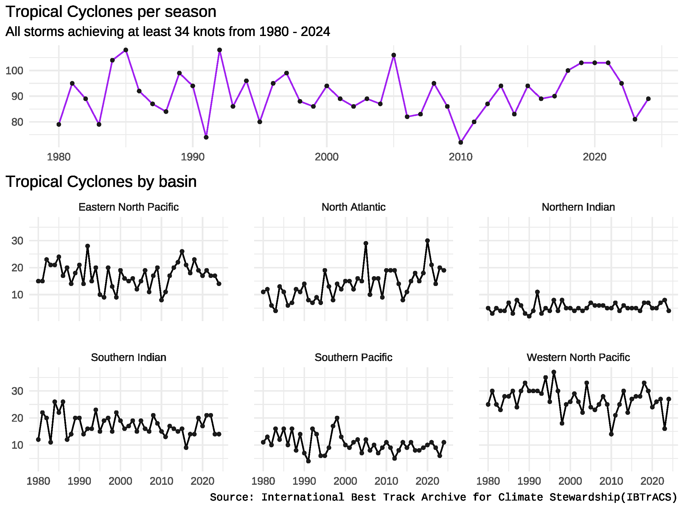
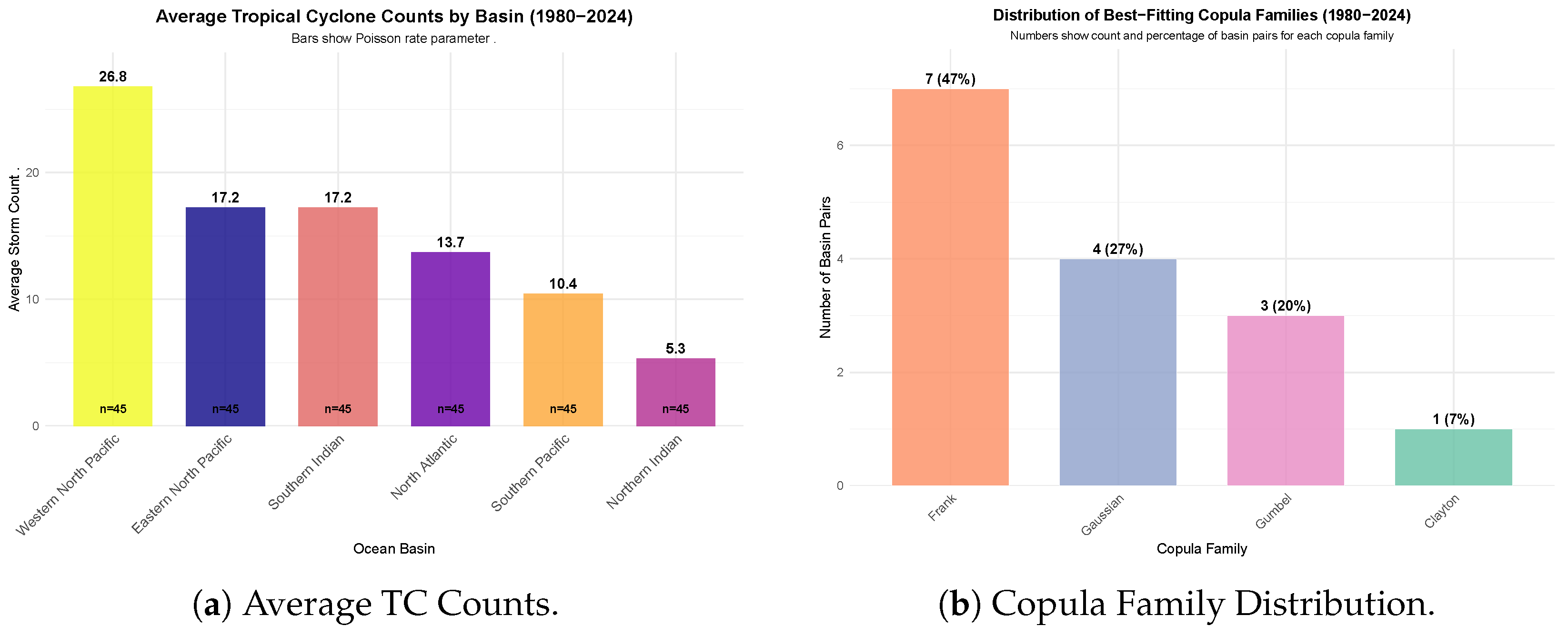
The Western North Pacific is the most active basin (average 26.8 storms/year), while the Northern Indian is the least active (5.3 storms/year). Substantial variability is evident: the North Atlantic ranges from 4 to 30 storms annually (see

Table 6. Summary statistics of annual TC counts by basin (1980–2024).

Basin	Mean	SD	Min	Max	Total	n
Eastern North Pacific	17.24	4.50	8	28	776	45
North Atlantic	13.71	5.52	4	30	617	45
Northern Indian	5.31	1.73	2	11	239	45
Southern Indian	17.24	3.78	9	26	776	45
Southern Pacific	10.42	3.43	4	20	469	45
Western North Pacific	26.78	4.54	14	37	1205	45

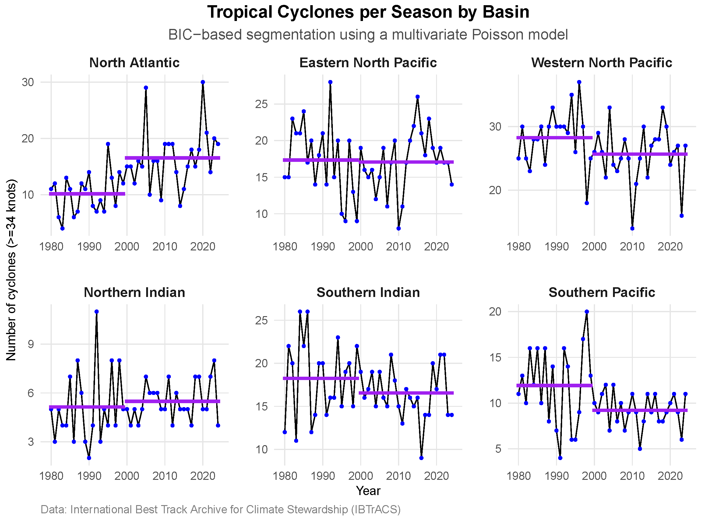
). Figure 3 shows the overall TC count trend over the year for total cyclone and for the basin-specific trend over the years from 1980 to 2024.

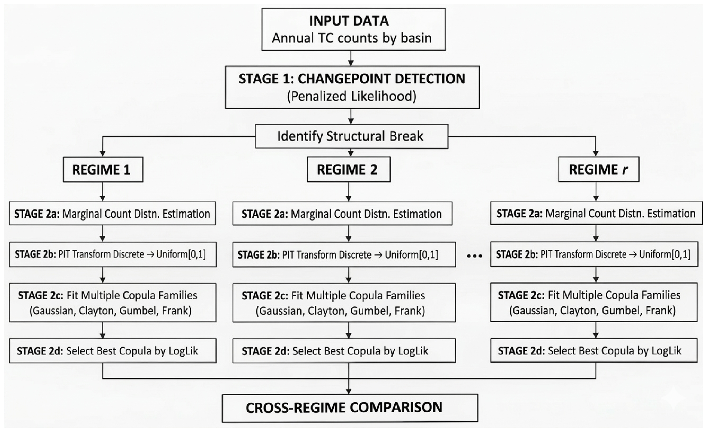
A key methodological innovation of this study is the pair-specific selection of the optimal copula family. Rather than imposing a single dependence structure on all basin pairs, we independently fit and compare four competing copula families (Gaussian, Clayton, Gumbel, Frank) for every pair of basins, and select the best one based on maximum log-likelihood. This approach is essential because the physical mechanisms linking tropical cyclone activity between different ocean basins can be fundamentally different. For example, some pairs may exhibit symmetric dependence (Gaussian or Frank), while others may show asymmetric tail dependence–lower-tail dependence (Clayton) indicating synchronized low-activity years, or upper-tail dependence (Gumbel) revealing concurrent extreme-storm seasons.

The results demonstrate that this flexibility is not merely theoretical. In the early regime (1980–1999), the Gaussian and Clayton copulas dominated, whereas the recent regime (2000–2024) shows a marked increase in the use of the Frank and Gumbel copulas. Such a shift would have been completely masked if a single copula family had been forced on all pairs. By allowing each pair to choose its own dependence structure, we aim to capture the true heterogeneity of global teleconnections and obtain a more flexible representation of how basin interactions have evolved under climate change. This pair-wise, regime-specific selection is a useful feature of our copula-based framework and provides a more nuanced picture than simpler correlation-based methods. We caveat that, given the regime sample sizes, the family selection itself should be read as exploratory.

4.2. Results Without Changepoint Detection (Single Period: 1980–2024)

To establish a baseline and quantify the improvement offered by incorporating non-stationarity, we first present the results for a stationary model that treats the entire 1980–2024 period as a single homogeneous regime. In this scenario, marginal Poisson parameters and bivariate copula dependencies are estimated once for the full 45-year duration. When analyzing the entire period as a single stationary regime, we find:

The Poisson rate parameters ($\lambda$) vary substantially across basins, with the Western North Pacific being the most active ($\lambda =26.78$) and the Northern Indian being the least active ($\lambda =5.31$).

The average Kendall’s $\tau$ across all basin pairs is $-0.019$, indicating weak overall dependence. Most dependencies are weak ($\left|\tau \right|<0.3$), with 53.3% of pairs showing positive dependence and 46.7% showing negative dependence.

The Frank copula dominates (46.7 ≈ 47 % of pairs), followed by Gaussian (26.7 ≈ 27%), Gumbel (20%), and Clayton (6.7 ≈ 7%). Figure 4 is a visual representation of family distribution.

This suggests primarily symmetric dependence structures with some evidence of upper-tail dependence. Strongest positive: Southern Indian vs. Western North Pacific ($\tau =0.236$, Gaussian copula); Strongest negative: Northern Indian vs. Western North Pacific ($\tau =-0.283$, Frank copula).

$${\mathbf{R}}_{\tau }^{\mathrm{full}}=\begin{array}{cc}& \begin{array}{cccccc}\mathrm{ENP}& \mathrm{NA}& \mathrm{NI}& \mathrm{SI}& \mathrm{SP}& \mathrm{WNP}\end{array}\\ \begin{array}{c}\mathrm{ENP}\\ \mathrm{NA}\\ \mathrm{NI}\\ \mathrm{SI}\\ \mathrm{SP}\\ \mathrm{WNP}\end{array}& \left(\begin{array}{cccccc}1& -0.168& 0.121& 0.119& 0.108& 0.126\\ -0.168& 1& 0.038& -0.059& -\mathbf{0}.\mathbf{202}& -0.113\\ 0.121& 0.038& 1& -0.206& 0.096& -\mathbf{0}.\mathbf{283}\\ 0.119& -0.059& -0.206& 1& 0.064& \mathbf{0}.\mathbf{236}\\ 0.108& \begin{array}{c}\hfill -\mathbf{0}.\mathbf{202}\end{array}& 0.096& 0.064& 1& -0.167\\ 0.126& -0.113& \begin{array}{c}\hfill -\mathbf{0}.\mathbf{283}\end{array}& \mathbf{0}.\mathbf{236}& -0.167& 1\end{array}\right)\end{array}.$$

(33)

To summarize the overall dependence structure when the whole 45-year period is treated as a single homogeneous regime, we construct the Kendall’s tau matrix ${\mathbf{R}}_{\tau }^{\mathrm{full}}$ from the copula-based estimates ${\tau }_C$ given in Table 7. For the six basins (ordered as: Eastern North Pacific (ENP), North Atlantic (NA), Northern Indian (NI), Southern Indian (SI), Southern Pacific (SP), Western North Pacific (WNP)), the matrix is in Equation (33).

Table 7. Copula results summary (without regime). Note: ${\tau }_C$ and $p_C$ refer to copula Kendall’s tau and its p-value; ${\tau }_O$ and $p_O$ refer to original Kendall’s tau and its p-value; $\Delta \tau$ is the change in tau (${\tau }_O-{\tau }_C$l); LL is log-likelihood; $p_{\mathrm{GOF}}$ is the GOF p-value. Significant p-values ($<0.05$) are in bold.

Basin 1	Basin 2	Copula	E. Par.	${\mathit{\tau }}_{\mathit{C}}$	${\mathit{p}}_{\mathit{C}}$	${\mathit{\tau }}_{\mathit{O}}$	${\mathit{p}}_{\mathit{O}}$	$\mathbf{\Delta }\mathit{\tau }$	LL	${\mathit{p}}_{\mathbf{GOF}}$
E. North Pacific	North Atlantic	Gaussian	−0.261	−0.168	0.007	−0.292	0.007	−0.124	3.381	0.774
E. North Pacific	Northern Indian	Gumbel	1.137	0.121	0.175	0.024	0.832	−0.097	1.426	0.833
E. North Pacific	Southern Indian	Frank	1.083	0.119	0.232	0.114	0.295	−0.005	0.694	0.128
E. North Pacific	Southern Pacific	Gumbel	1.121	0.108	0.176	0.076	0.489	−0.032	1.019	0.755
E. North Pacific	W. North Pacific	Clayton	0.289	0.126	0.069	0.102	0.352	−0.024	2.009	0.971
North Atlantic	Northern Indian	Frank	0.342	0.038	0.692	0.098	0.387	0.060	0.078	0.931
North Atlantic	Southern Indian	Frank	−0.534	−0.059	0.495	−0.092	0.401	−0.033	0.232	0.696
North Atlantic	Southern Pacific	Frank	−1.882	−0.202	0.014	−0.223	0.042	−0.021	2.726	0.284
North Atlantic	W. North Pacific	Gaussian	−0.177	−0.113	0.096	−0.190	0.082	−0.077	1.336	0.147
Northern Indian	Southern Indian	Gaussian	−0.317	−0.206	0.089	−0.140	0.222	0.066	1.013	0.500
Northern Indian	Southern Pacific	Gumbel	1.106	0.096	0.257	−0.036	0.754	−0.132	0.760	0.088
Northern Indian	W. North Pacific	Frank	−2.725	−0.283	0.014	−0.175	0.127	0.108	1.931	0.069
Southern Indian	Southern Pacific	Frank	0.578	0.064	0.535	0.082	0.458	0.018	0.191	0.284
Southern Indian	W. North Pacific	Gaussian	0.362	0.236	0.015	0.220	0.046	-0.016	2.148	0.833
Southern Pacific	W. North Pacific	Frank	−1.537	−0.167	0.141	−0.162	0.142	0.005	0.974	0.167

Table 7. Copula results summary (without regime). Note: ${\tau }_C$ and $p_C$ refer to copula Kendall’s tau and its p-value; ${\tau }_O$ and $p_O$ refer to original Kendall’s tau and its p-value; $\Delta \tau$ is the change in tau (${\tau }_O-{\tau }_C$l); LL is log-likelihood; $p_{\mathrm{GOF}}$ is the GOF p-value. Significant p-values ($<0.05$) are in bold.

Basin 1	Basin 2	Copula	E. Par.	${\mathit{\tau }}_{\mathit{C}}$	${\mathit{p}}_{\mathit{C}}$	${\mathit{\tau }}_{\mathit{O}}$	${\mathit{p}}_{\mathit{O}}$	$\mathbf{\Delta }\mathit{\tau }$	LL	${\mathit{p}}_{\mathbf{GOF}}$
E. North Pacific	North Atlantic	Gaussian	−0.261	−0.168	0.007	−0.292	0.007	−0.124	3.381	0.774
E. North Pacific	Northern Indian	Gumbel	1.137	0.121	0.175	0.024	0.832	−0.097	1.426	0.833
E. North Pacific	Southern Indian	Frank	1.083	0.119	0.232	0.114	0.295	−0.005	0.694	0.128
E. North Pacific	Southern Pacific	Gumbel	1.121	0.108	0.176	0.076	0.489	−0.032	1.019	0.755
E. North Pacific	W. North Pacific	Clayton	0.289	0.126	0.069	0.102	0.352	−0.024	2.009	0.971
North Atlantic	Northern Indian	Frank	0.342	0.038	0.692	0.098	0.387	0.060	0.078	0.931
North Atlantic	Southern Indian	Frank	−0.534	−0.059	0.495	−0.092	0.401	−0.033	0.232	0.696
North Atlantic	Southern Pacific	Frank	−1.882	−0.202	0.014	−0.223	0.042	−0.021	2.726	0.284
North Atlantic	W. North Pacific	Gaussian	−0.177	−0.113	0.096	−0.190	0.082	−0.077	1.336	0.147
Northern Indian	Southern Indian	Gaussian	−0.317	−0.206	0.089	−0.140	0.222	0.066	1.013	0.500
Northern Indian	Southern Pacific	Gumbel	1.106	0.096	0.257	−0.036	0.754	−0.132	0.760	0.088
Northern Indian	W. North Pacific	Frank	−2.725	−0.283	0.014	−0.175	0.127	0.108	1.931	0.069
Southern Indian	Southern Pacific	Frank	0.578	0.064	0.535	0.082	0.458	0.018	0.191	0.284
Southern Indian	W. North Pacific	Gaussian	0.362	0.236	0.015	0.220	0.046	-0.016	2.148	0.833
Southern Pacific	W. North Pacific	Frank	−1.537	−0.167	0.141	−0.162	0.142	0.005	0.974	0.167

The average absolute off-diagonal entry is $|\overline{\tau }|=0.14$, indicating generally weak dependencies. The most notable positive link is between the Southern Indian and Western North Pacific ($\tau =0.236$), while the strongest negative relationship is between the Northern Indian and Western North Pacific ($\tau =-0.283$). This matrix will serve as a benchmark for the regime-specific matrices obtained after accounting for the 2000 changepoint.

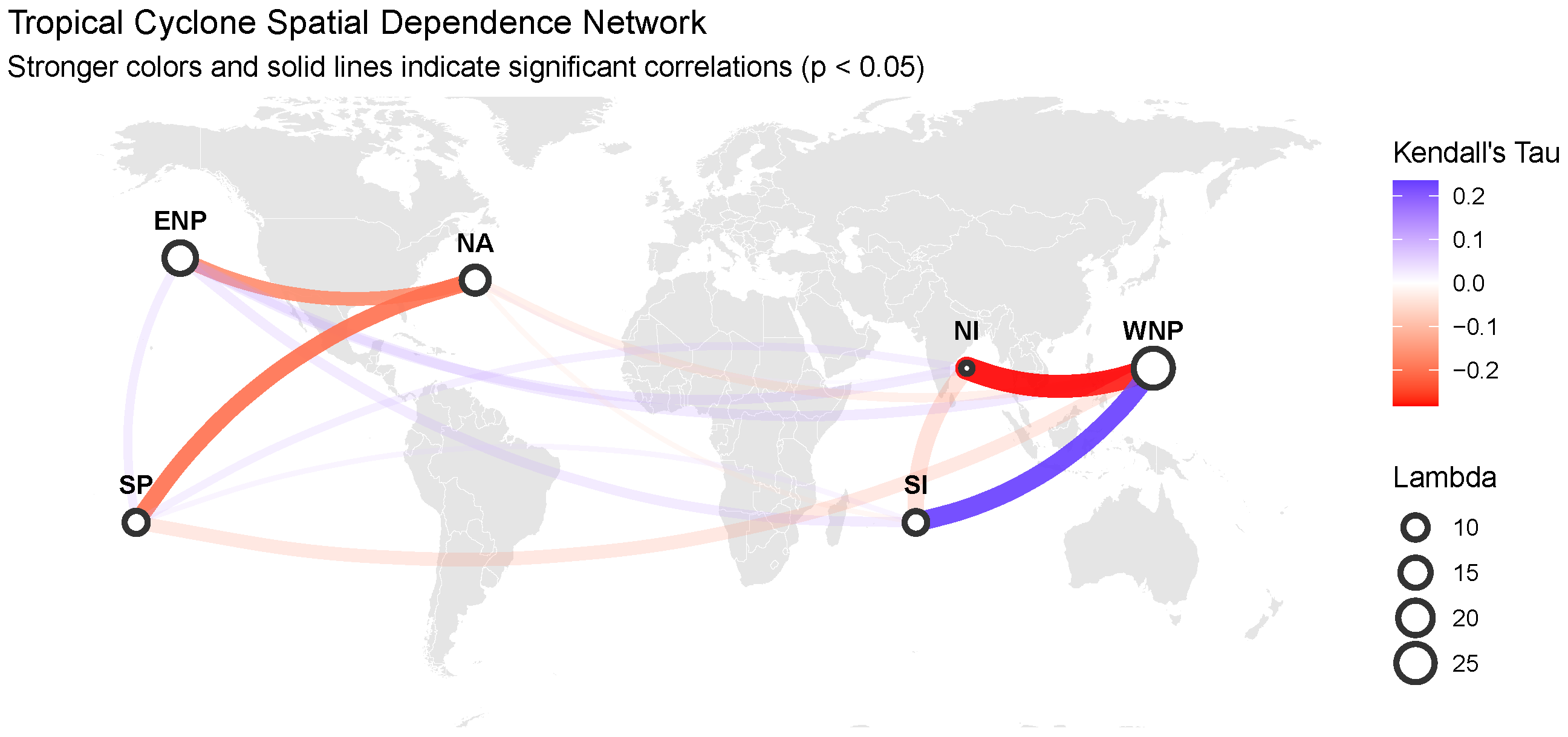
Here, Figure 5 shows the global tropical cyclone basin dependence network for 1980–2024 based on the copula-based dependencies or correlation ${\tau }_c$. Significant correlations ($p<0.05$) are represented by solid, deep-colored lines; these correspond to entries where the p-value ($p_C$) is in bold. The blurred or faint lines indicate that while a relationship might exist, it is not statistically significant at the 95% confidence level. Red lines indicate a negative correlation (as storm counts in one basin increase, they tend to decrease in the other). Blue lines indicate a positive correlation (storm counts in both basins tend to increase or decrease together).

Significant negative dependencies (strong red lines): E. North Pacific (ENP) and North Atlantic (NA) show a significant negative dependency (${\tau }_C=-0.168,p_C=0.007$). This is shown as the prominent red arc connecting the two basins in the Western Hemisphere. The North Atlantic (NA) and Southern Pacific (SP) pair shows a significant negative correlation (${\tau }_C=-0.202,p_C=0.014$). Northern Indian (NI) and W. North Pacific (WNP)—this pair also exhibits a strong significant negative dependency (${\tau }_C=-0.283,p_C=0.014$). Significant positive dependency (strong blue line): Southern Indian (SI) and W. North Pacific (WNP) show a key positive relationship (${\tau }_C=0.236,p_C=0.015$). In Figure 5, this is represented by the deep blue line in the Eastern Hemisphere, indicating that these basins often see synchronized storm activity. This plot can be explained by stating that the global dependency network is dominated by negative regional correlations across the North Atlantic and Pacific, while the Western North Pacific acts as a central hub showing both strong positive dependency with the Southern Indian basin and negative dependency with the Northern Indian basin.

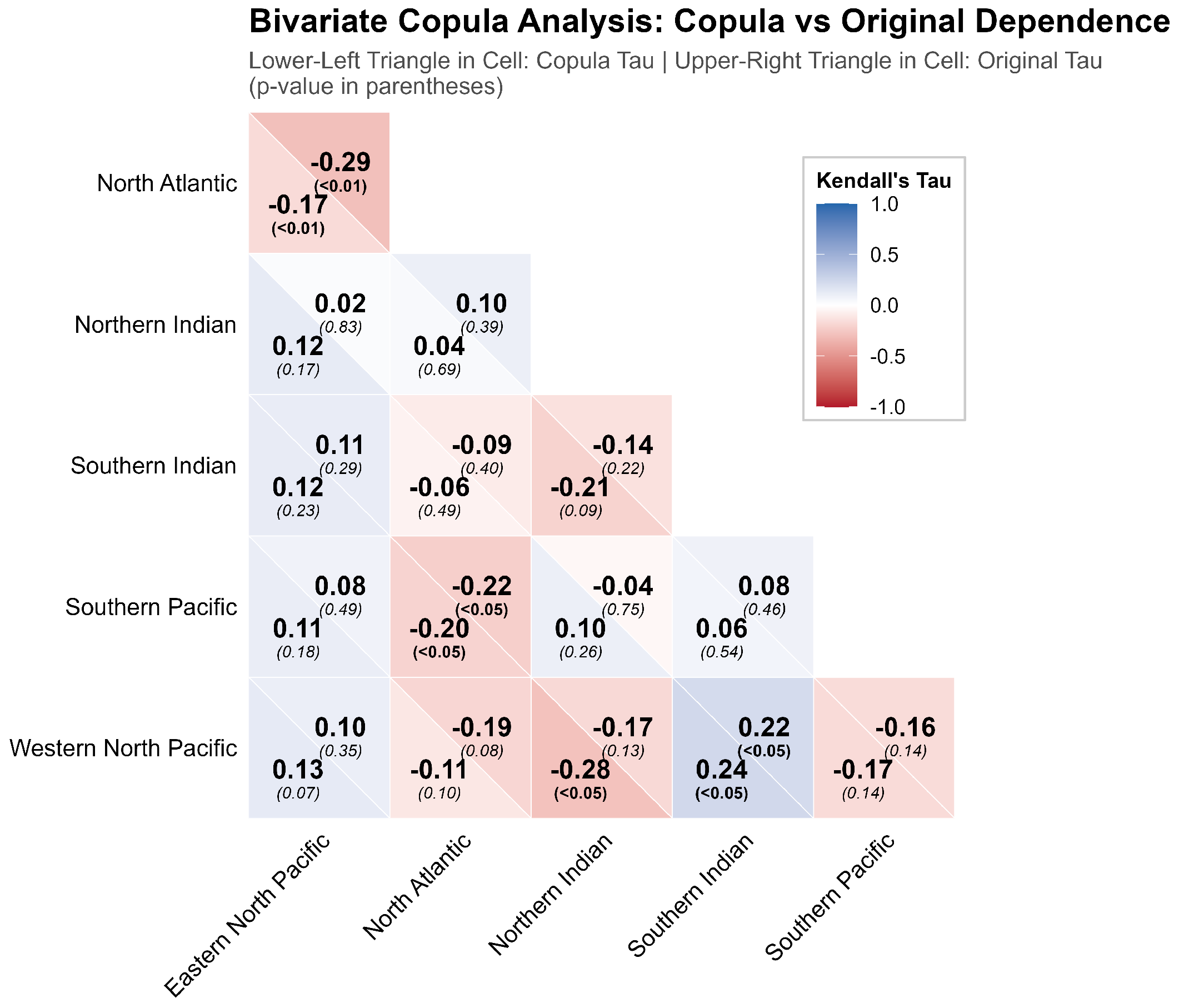
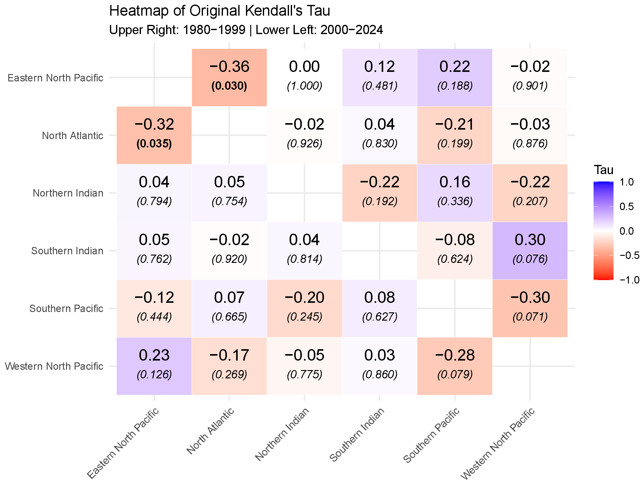
While the regional Dependence Network provides a visual overview of global correlations, the Bivariate Heatmap (Figure 6) confirms these relationships by comparing Copula Tau (${\tau }_C$) against Original Tau (${\tau }_O$), highlighting that the copula approach captures significant dependencies, such as the −0.28 correlation between the Northern Indian and W. North Pacific basins that traditional correlation methods fail to detect at the 95% confidence level. Also, the Southern Pacific and Northern Indian basins shows opposite dependencies for the copula and original data, even though neither of the values is statistically significant at a 95% confidence level.

The stationary model’s limitations become apparent when examining specific pairs. For instance, the Northern Indian–Southern Pacific pair shows a weak, non-significant positive dependence (${\tau }_C=0.096,p_C=0.257$) in the aggregate analysis. However, as we will show in Section 4.2, this masks a dramatic reversal: a weak positive relationship in 1980–1999 (${\tau }_C=0.209,p_C=0.066$) transforms into a remarkably strong negative dependence in 2000–2024 (${\tau }_C=-0.464,p_C<0.001$). The stationary analysis also misrepresents the nature of the dependence structures. With 46.7% Frank copulas and 26.7% Gaussian copulas, the aggregate analysis suggests predominantly symmetric, weak dependencies. This obscures the emergence of tail dependence in the recent regime, where Gumbel copulas (capturing joint extreme events) appear in 20% of pairs compared to only 7% in 1980–1999.

The values reported at Table 7 are from a single randomized-PIT realization. A $B_{\mathrm{MC}}=500$ averaging run reproduces every ${\widehat{\tau }}_C$ within $\pm 0.04$ and every modal copula family unchanged; across-replication standard deviations are ≤0.04 for all 15 pairs presented at Table A1 for robustness.

4.3. Results with Changepoint Detection (Two Regimes: 1980–1999 and 2000–2024)

The changepoint analysis identifies the year 2000 as a significant structural break, dividing the data into two distinct climate regimes. Figure 7 shows the TC count trend over the year for the basin-specific trend after determining the change point at 2000.

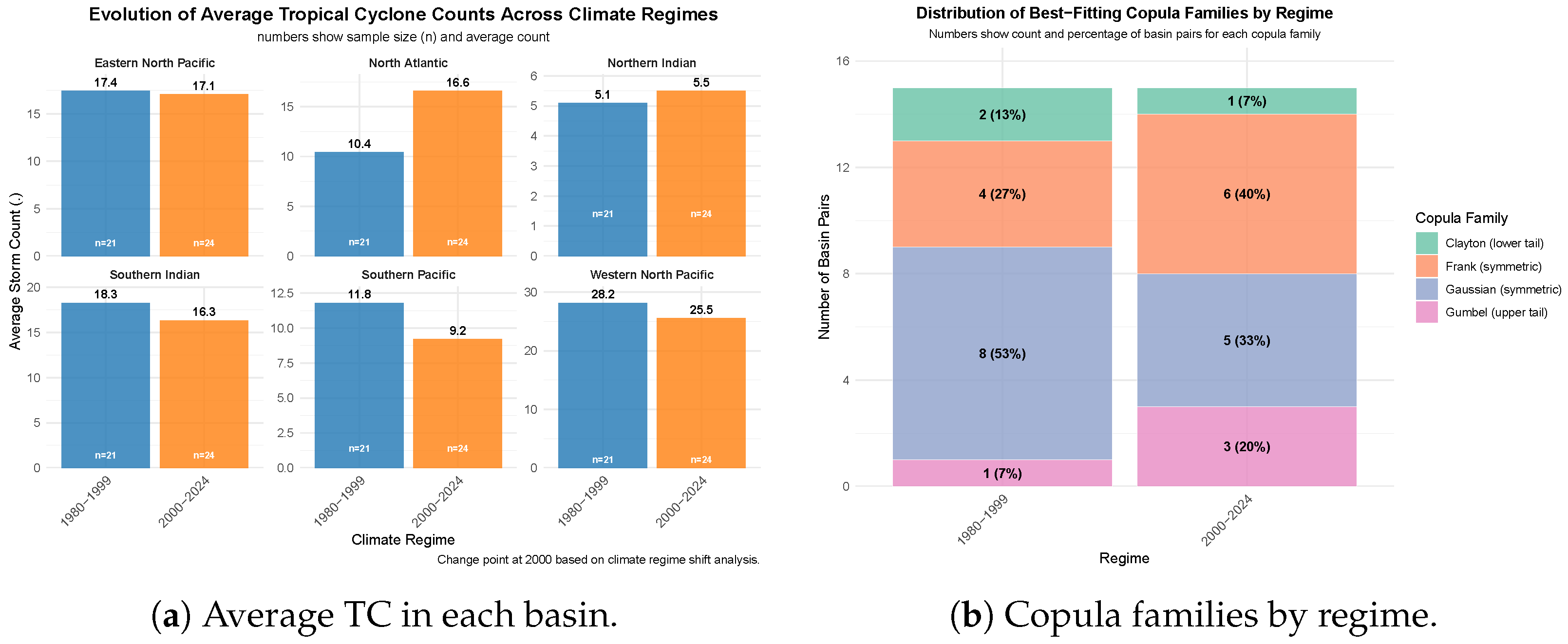
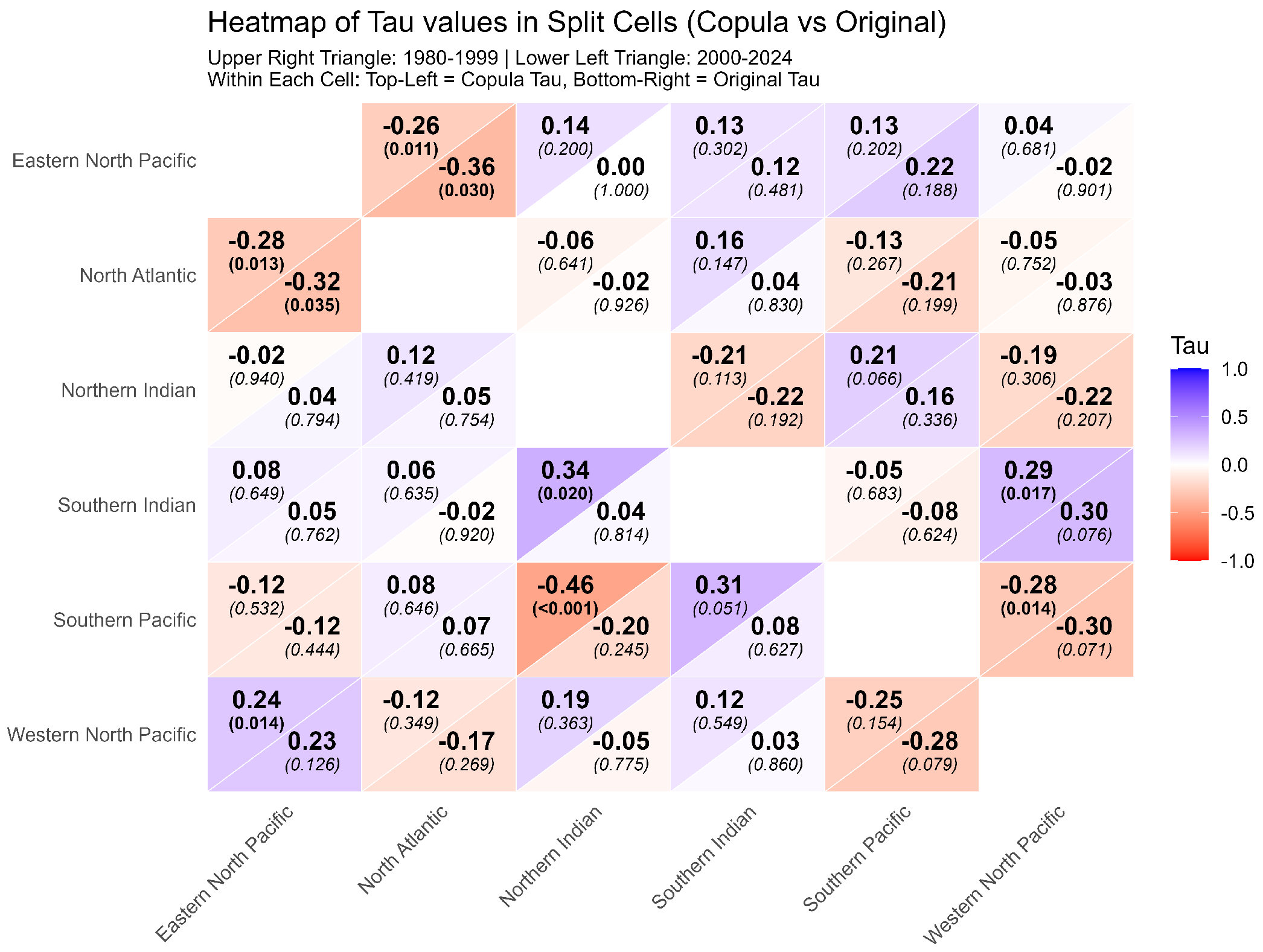
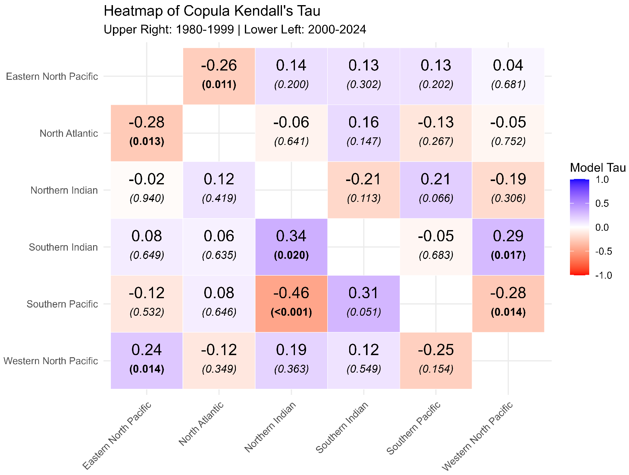
Figure 4 and Figure 8 show the marginal mean TC and copula family distribution for all basins for both cases, with and without a changepoint. Figure 6 and Figure 9, Figure 10 and Figure 11 represent the $\tau$ values with the p-value of each $\tau$ for no changepoint, and with changepoint. The goodness-of-fit p-values reported in Table 8 for the stationary analysis) confirm that the selected copulas generally provide an adequate representation of the dependence structure. For the vast majority of basin pairs in both regimes, the p-value exceeds 0.05, meaning that the chosen copula family cannot be rejected at conventional significance levels (see Table 8). For instance, in the 2000–2024 regime, 14 out of 15 pairs have p-values above 0.05, with only the North Atlantic–Western North Pacific pair showing a borderline value of 0.049. This occasional low p-value may reflect the limited sample size (24 years) or the inherent difficulty of capturing complex dependence with a simple one-parameter family, but overall, the GOF results lend strong support to our model selections. The generally high p-values across all pairs and regimes demonstrate that the combination of the probability integral transform (PIT) and the subsequent copula fitting yields statistically defensible models for the observed tropical cyclone counts.

Table 8. Comparison of copula results across two regimes (1980–1999 and 2000–2024). Note: ${\tau }_C$ and $p_C$ refer to copula Kendall’s tau and its p-value; ${\tau }_O$ and $p_O$ refer to original Kendall’s tau and its p-value; $\Delta \tau$ is the change in tau; LL is log-likelihood; $p_{\mathrm{GOF}}$ is the GOF p-value. Significant p-values (<$0.05$) are in bold.

Basin 1	Basin 2	Copula	E. Par.	${\mathit{\tau }}_{\mathit{C}}$	${\mathit{p}}_{\mathit{C}}$	${\mathit{\tau }}_{\mathit{O}}$	${\mathit{p}}_{\mathit{O}}$	$\mathbf{\Delta }\mathit{\tau }$	LL	${\mathit{p}}_{\mathbf{GOF}}$
Regime 1: 1980–1999
E. North Pacific	North Atlantic	Gaussian	−0.393	−0.257	0.011	−0.359	0.030	−0.102	2.601	0.794
E. North Pacific	Northern Indian	Gumbel	1.160	0.138	0.200	0.000	1.000	−0.138	1.380	0.598
E. North Pacific	Southern Indian	Frank	1.167	0.128	0.302	0.117	0.481	−0.011	0.524	0.794
E. North Pacific	Southern Pacific	Gaussian	0.197	0.126	0.203	0.217	0.188	0.091	0.777	0.676
E. North Pacific	W. North Pacific	Clayton	0.091	0.043	0.681	−0.021	0.901	−0.064	0.089	0.931
North Atlantic	Northern Indian	Gaussian	−0.099	−0.063	0.641	−0.016	0.926	0.047	0.107	0.735
North Atlantic	Southern Indian	Clayton	0.375	0.158	0.147	0.036	0.830	−0.122	1.033	0.971
North Atlantic	Southern Pacific	Frank	−1.218	−0.133	0.267	−0.213	0.199	−0.080	0.597	0.990
North Atlantic	W. North Pacific	Gaussian	−0.075	−0.048	0.752	−0.026	0.876	0.022	0.049	0.833
Northern Indian	Southern Indian	Gaussian	−0.318	−0.206	0.113	−0.224	0.192	−0.018	1.031	0.774
Northern Indian	Southern Pacific	Gaussian	0.323	0.209	0.066	0.164	0.336	−0.045	1.440	0.637
Northern Indian	W. North Pacific	Frank	−1.767	−0.191	0.306	−0.219	0.207	−0.028	0.432	0.500
Southern Indian	Southern Pacific	Frank	−0.425	−0.047	0.683	−0.081	0.624	−0.034	0.083	0.755
Southern Indian	W. North Pacific	Gaussian	0.445	0.294	0.017	0.301	0.076	0.007	1.868	0.951
Southern Pacific	W. North Pacific	Gaussian	−0.429	−0.283	0.014	−0.304	0.071	−0.021	2.176	0.147
Regime 2: 2000–2024
E. North Pacific	North Atlantic	Frank	−2.684	−0.279	0.013	−0.324	0.035	−0.045	2.403	0.284
E. North Pacific	Northern Indian	Gaussian	−0.035	−0.022	0.940	0.042	0.794	0.064	0.003	0.912
E. North Pacific	Southern Indian	Frank	0.721	0.080	0.649	0.047	0.762	−0.033	0.101	0.128
E. North Pacific	Southern Pacific	Gaussian	−0.193	−0.124	0.531	−0.121	0.444	0.003	0.167	0.539
E. North Pacific	W. North Pacific	Clayton	0.626	0.238	0.014	0.234	0.126	−0.004	3.236	0.853
North Atlantic	Northern Indian	Gaussian	0.182	0.116	0.419	0.051	0.754	−0.065	0.302	0.480
North Atlantic	Southern Indian	Gaussian	0.094	0.060	0.635	−0.016	0.920	−0.076	0.111	0.578
North Atlantic	Southern Pacific	Frank	0.707	0.078	0.646	0.069	0.664	−0.009	0.103	0.833
North Atlantic	W. North Pacific	Frank	−1.139	−0.125	0.349	−0.169	0.269	−0.044	0.419	0.049
Northern Indian	Southern Indian	Gumbel	1.526	0.345	0.020	0.039	0.814	−0.306	1.179	0.951
Northern Indian	Southern Pacific	Gaussian	−0.666	−0.464	<0.001	−0.195	0.245	0.269	2.021	0.892
Northern Indian	W. North Pacific	Gumbel	1.230	0.187	0.363	−0.046	0.775	−0.233	0.277	0.500
Southern Indian	Southern Pacific	Gumbel	1.453	0.312	0.051	0.078	0.627	−0.234	0.908	0.853
Southern Indian	W. North Pacific	Frank	1.064	0.117	0.549	0.027	0.860	−0.090	0.163	0.245
Southern Pacific	W. North Pacific	Frank	−2.337	−0.247	0.154	−0.277	0.079	−0.030	0.675	0.774

Table 8. Comparison of copula results across two regimes (1980–1999 and 2000–2024). Note: ${\tau }_C$ and $p_C$ refer to copula Kendall’s tau and its p-value; ${\tau }_O$ and $p_O$ refer to original Kendall’s tau and its p-value; $\Delta \tau$ is the change in tau; LL is log-likelihood; $p_{\mathrm{GOF}}$ is the GOF p-value. Significant p-values (<$0.05$) are in bold.

Basin 1	Basin 2	Copula	E. Par.	${\mathit{\tau }}_{\mathit{C}}$	${\mathit{p}}_{\mathit{C}}$	${\mathit{\tau }}_{\mathit{O}}$	${\mathit{p}}_{\mathit{O}}$	$\mathbf{\Delta }\mathit{\tau }$	LL	${\mathit{p}}_{\mathbf{GOF}}$
Regime 1: 1980–1999
E. North Pacific	North Atlantic	Gaussian	−0.393	−0.257	0.011	−0.359	0.030	−0.102	2.601	0.794
E. North Pacific	Northern Indian	Gumbel	1.160	0.138	0.200	0.000	1.000	−0.138	1.380	0.598
E. North Pacific	Southern Indian	Frank	1.167	0.128	0.302	0.117	0.481	−0.011	0.524	0.794
E. North Pacific	Southern Pacific	Gaussian	0.197	0.126	0.203	0.217	0.188	0.091	0.777	0.676
E. North Pacific	W. North Pacific	Clayton	0.091	0.043	0.681	−0.021	0.901	−0.064	0.089	0.931
North Atlantic	Northern Indian	Gaussian	−0.099	−0.063	0.641	−0.016	0.926	0.047	0.107	0.735
North Atlantic	Southern Indian	Clayton	0.375	0.158	0.147	0.036	0.830	−0.122	1.033	0.971
North Atlantic	Southern Pacific	Frank	−1.218	−0.133	0.267	−0.213	0.199	−0.080	0.597	0.990
North Atlantic	W. North Pacific	Gaussian	−0.075	−0.048	0.752	−0.026	0.876	0.022	0.049	0.833
Northern Indian	Southern Indian	Gaussian	−0.318	−0.206	0.113	−0.224	0.192	−0.018	1.031	0.774
Northern Indian	Southern Pacific	Gaussian	0.323	0.209	0.066	0.164	0.336	−0.045	1.440	0.637
Northern Indian	W. North Pacific	Frank	−1.767	−0.191	0.306	−0.219	0.207	−0.028	0.432	0.500
Southern Indian	Southern Pacific	Frank	−0.425	−0.047	0.683	−0.081	0.624	−0.034	0.083	0.755
Southern Indian	W. North Pacific	Gaussian	0.445	0.294	0.017	0.301	0.076	0.007	1.868	0.951
Southern Pacific	W. North Pacific	Gaussian	−0.429	−0.283	0.014	−0.304	0.071	−0.021	2.176	0.147
Regime 2: 2000–2024
E. North Pacific	North Atlantic	Frank	−2.684	−0.279	0.013	−0.324	0.035	−0.045	2.403	0.284
E. North Pacific	Northern Indian	Gaussian	−0.035	−0.022	0.940	0.042	0.794	0.064	0.003	0.912
E. North Pacific	Southern Indian	Frank	0.721	0.080	0.649	0.047	0.762	−0.033	0.101	0.128
E. North Pacific	Southern Pacific	Gaussian	−0.193	−0.124	0.531	−0.121	0.444	0.003	0.167	0.539
E. North Pacific	W. North Pacific	Clayton	0.626	0.238	0.014	0.234	0.126	−0.004	3.236	0.853
North Atlantic	Northern Indian	Gaussian	0.182	0.116	0.419	0.051	0.754	−0.065	0.302	0.480
North Atlantic	Southern Indian	Gaussian	0.094	0.060	0.635	−0.016	0.920	−0.076	0.111	0.578
North Atlantic	Southern Pacific	Frank	0.707	0.078	0.646	0.069	0.664	−0.009	0.103	0.833
North Atlantic	W. North Pacific	Frank	−1.139	−0.125	0.349	−0.169	0.269	−0.044	0.419	0.049
Northern Indian	Southern Indian	Gumbel	1.526	0.345	0.020	0.039	0.814	−0.306	1.179	0.951
Northern Indian	Southern Pacific	Gaussian	−0.666	−0.464	<0.001	−0.195	0.245	0.269	2.021	0.892
Northern Indian	W. North Pacific	Gumbel	1.230	0.187	0.363	−0.046	0.775	−0.233	0.277	0.500
Southern Indian	Southern Pacific	Gumbel	1.453	0.312	0.051	0.078	0.627	−0.234	0.908	0.853
Southern Indian	W. North Pacific	Frank	1.064	0.117	0.549	0.027	0.860	−0.090	0.163	0.245
Southern Pacific	W. North Pacific	Frank	−2.337	−0.247	0.154	−0.277	0.079	−0.030	0.675	0.774

For multiple-testing considerations, with 15 basin pairs per regime, we view the analysis as exploratory. We report the unadjusted p-values shown in Table 8 (consistent with standard practice in copula-based exploratory studies) as the primary inference, and supplement them with Benjamini–Hochberg false-discovery-rate adjustment [34] as a sensitivity check. At the moderate exploratory threshold $q=0.10$, all seven headline findings retain significance: in Regime 1, ENP–NA, SP–WNP, and SI–WNP; in Regime 2, NI–SP, ENP–NA, ENP–WNP, and NI–SI. At the stricter $q=0.05$, only NI–SP (Regime 2, $p_C<0.001$) retains formal significance, which is the expected behavior given the regime sample sizes ($n_1=20,n_2=25$) and the multiplicity of tests; this is therefore framed as a power constraint rather than as evidence against the reported relationships. The principal evidence supporting the regime decomposition is the effect-size stability across nearby break years (

Table 9. Stage 2 sensitivity to the break year. For each candidate $\nu \in \{1998,\dots ,2002\}$, we report the three principal findings and verify their stability.

Break Year $\mathit{\nu }$	1998	1999	2000	2001	2002
NA mean increase %	64.4%	61.8%	59.4%	59.0%	56.6%
NA–ENP ${\widehat{\tau }}_C$ R1	$-0.303$	$-0.327$	$-\mathbf{0}.\mathbf{314}$	$-0.285$	$-0.286$
NA–ENP ${\widehat{\tau }}_C$ R2	$-0.175$	$-0.202$	$-\mathbf{0}.\mathbf{280}$	$-0.262$	$-0.261$
NI–SP ${\widehat{\tau }}_C$ R2	$-0.114$	$-0.497$	$-\mathbf{0}.\mathbf{463}$	$-0.487$	$-0.493$

Note: Values in bold indicate the results corresponding to the primary detected changepoint year ($\nu =2000$) used in the model analysis.

).

We can check the sensitivity to nearby break years. To verify that the substantive conclusions do not hinge on the exact break at $\nu =2000$, we re-ran Stage 2 with $\nu \in \{1998,1999,2000,2001,2002\}$ (see Table 9). For each candidate, the principal qualitative results: (i) around 60% increase in NA mean intensity, (ii) the persistent NA–ENP negative link with ${\widehat{\tau }}_C\in [-0.33,-0.24]$ in regime 1 (R1) and ${\widehat{\tau }}_C\in [-0.28,-0.18]$ in regime 2 (R2), and (iii) the emergence of a strong negative NI–SP link in the recent regime mostly (${\widehat{\tau }}_C\in [-0.50,-0.45]$), remain stable, supporting the robustness of the regime decomposition.

The within-regime residual and i.i.d. diagnostics in the Stage 2 inference assume that, within each regime, the $(X_{ir}^t,X_{jr}^t)$ observations are i.i.d. To assess this, we computed (i) Pearson and Anscombe Poisson residuals per basin per regime, (ii) the autocorrelation function of the residuals at lags 1–6, and (iii) the weighted-portmanteau test of [38].

As numerical evidence for the sensitivity statements, Table 9 and Table 12 report the actual BIC profile and the Stage 2 sensitivity to the break-year choice and Table 13 summaries the residual diagnostics and the ${\Delta }_{\mathrm{LL}}^{\left(ij\right)}$ corroboration (Table 10), neither of which depends on the p-value cutoff.

Marginal Distribution Changes: Table 11 shows substantial shifts in tropical cyclone activity between regimes. The North Atlantic exhibits the most dramatic increase (59%), while the Southern Pacific shows a significant decrease (22%). The Western North Pacific (WNP), while remaining dominant, decreased by 9.4%. This reduction aligns with observed interdecadal changes in WNP activity linked to the Pacific Decadal Oscillation (PDO) phase shift. These marginal changes alone underscore the system’s non-stationarity and motivate the need for regime-specific dependence analysis.

The largest absolute lag-1 residual ACF across the $6\times 2=12$ basin/regime combinations is $0.36$ (Eastern North Pacific, regime 2; the next-largest values are the Northern Indian regime 1 at $-0.28$ and Southern Indian regime 1 at $-0.24$), and no portmanteau p-value falls below $0.05$ after Benjamini–Hochberg correction (see Table 13). We caveat that the regime lengths ($n_1=20$, $n_2=25$) limit the power to detect serial dependence, so absence of evidence is not evidence of absence. Extending the framework to AR(1)-driven Gaussian latent processes, as developed in [21,39] is the natural next step and is identified as future work.

Table 10. With regime vs. no-regime corroboration. Positive ${\Delta }_{\mathrm{LL}}^{\left(ij\right)}$ indicates that the joint copula log-likelihood improves under the year-2000 split; positive $\Delta {\mathrm{BIC}}^{\left(ij\right)}$ (in bold) means the improvement survives the BIC penalty.

Basin 1	Basin 2	${\mathbf{\Delta }}_{\mathbf{LL}}^{\left(\mathit{ij}\right)}$	$\mathbf{\Delta }{\mathbf{BIC}}^{\left(\mathit{ij}\right)}$
Eastern North Pacific	North Atlantic	19.23	27.03
Eastern North Pacific	Northern Indian	0.18	−11.06
Eastern North Pacific	Southern Indian	1.05	−9.33
Eastern North Pacific	Southern Pacific	4.32	−2.78
Eastern North Pacific	Western North Pacific	2.84	−5.73
North Atlantic	Northern Indian	16.82	22.22
North Atlantic	Southern Indian	17.80	24.19
North Atlantic	Southern Pacific	19.45	27.48
North Atlantic	Western North Pacific	17.41	23.39
Northern Indian	Southern Indian	1.24	−8.94
Northern Indian	Southern Pacific	5.04	−1.35
Northern Indian	Western North Pacific	1.47	−8.47
Southern Indian	Southern Pacific	4.86	−1.70
Southern Indian	Western North Pacific	2.37	−6.68
Southern Pacific	Western North Pacific	6.83	2.25

Note: Values in bold indicate that the improvement survives the BIC penalty (positive $\Delta {\mathrm{BIC}}^{\left(ij\right)}$).

Table 10. With regime vs. no-regime corroboration. Positive ${\Delta }_{\mathrm{LL}}^{\left(ij\right)}$ indicates that the joint copula log-likelihood improves under the year-2000 split; positive $\Delta {\mathrm{BIC}}^{\left(ij\right)}$ (in bold) means the improvement survives the BIC penalty.

Basin 1	Basin 2	${\mathbf{\Delta }}_{\mathbf{LL}}^{\left(\mathit{ij}\right)}$	$\mathbf{\Delta }{\mathbf{BIC}}^{\left(\mathit{ij}\right)}$
Eastern North Pacific	North Atlantic	19.23	27.03
Eastern North Pacific	Northern Indian	0.18	−11.06
Eastern North Pacific	Southern Indian	1.05	−9.33
Eastern North Pacific	Southern Pacific	4.32	−2.78
Eastern North Pacific	Western North Pacific	2.84	−5.73
North Atlantic	Northern Indian	16.82	22.22
North Atlantic	Southern Indian	17.80	24.19
North Atlantic	Southern Pacific	19.45	27.48
North Atlantic	Western North Pacific	17.41	23.39
Northern Indian	Southern Indian	1.24	−8.94
Northern Indian	Southern Pacific	5.04	−1.35
Northern Indian	Western North Pacific	1.47	−8.47
Southern Indian	Southern Pacific	4.86	−1.70
Southern Indian	Western North Pacific	2.37	−6.68
Southern Pacific	Western North Pacific	6.83	2.25

Note: Values in bold indicate that the improvement survives the BIC penalty (positive $\Delta {\mathrm{BIC}}^{\left(ij\right)}$).

Table 11. Poisson rate parameters ($\lambda$) for tropical cyclone counts by basin and regime.

Basin	1980–1999	2000–2024	Change (%)
Eastern North Pacific	17.43	17.08	−2.0%
North Atlantic	10.43	16.58	+59.0%
Northern Indian	5.10	5.50	+7.8%
Southern Indian	18.29	16.33	−10.7%
Southern Pacific	11.81	9.21	−22.0%
Western North Pacific	28.19	25.54	−9.4%

Table 11. Poisson rate parameters ($\lambda$) for tropical cyclone counts by basin and regime.

Basin	1980–1999	2000–2024	Change (%)
Eastern North Pacific	17.43	17.08	−2.0%
North Atlantic	10.43	16.58	+59.0%
Northern Indian	5.10	5.50	+7.8%
Southern Indian	18.29	16.33	−10.7%
Southern Pacific	11.81	9.21	−22.0%
Western North Pacific	28.19	25.54	−9.4%

Table 12. Stage 1 BIC profile across one-changepoint configurations $\nu \in \{1990,\dots ,2010\}$ for the joint $d=6$-variate Poisson–Gaussian-copula model, expressed under the Lund-consistent indexing convention in which $\nu =y$ denotes year y as the first year of the new regime. The minimum is at $\widehat{\nu }=2000$, exactly matching the genetic-algorithm result of Lund et al. [21] and the manuscript’s headline split (1980–1999 vs. 2000–2024). Results for 2000 (detected CP) are highlighted in bold.

Year $\mathit{\nu }$	Chpts Index	BIC	$\mathbf{\Delta }\mathbf{BIC}$	Rank
1990	11	1542.93	26.33	9
1995	16	1530.48	13.88	6
1998	19	1531.96	15.36	7
1999	20	1524.46	7.86	5
2000	21	1516.60	0.00	1
2001	22	1519.85	3.25	2
2002	23	1520.01	3.41	3
2005	26	1523.38	6.78	4
2010	31	1533.60	17.00	8

Note: The row highlighted in bold indicates the optimal one-changepoint configuration ($\widehat{\nu }=2000$) minimizing the BIC criterion (Rank 1). Assigns years 1980–1999 ($t=1,\dots ,20$) to regime 1 and years 2000–2024 ($t=21,\dots ,45$) to regime 2; this is the convention used by joint_distro_code.R and Lund (2025). The BIC sensitivity band ($\Delta \mathrm{BIC}\le 7$) covers $\{2000,2001,2002,2005\}$; outside this band, the BIC penalty is markedly larger. Stage-2 substantive findings are stable across this band (Table 9).

Table 12. Stage 1 BIC profile across one-changepoint configurations $\nu \in \{1990,\dots ,2010\}$ for the joint $d=6$-variate Poisson–Gaussian-copula model, expressed under the Lund-consistent indexing convention in which $\nu =y$ denotes year y as the first year of the new regime. The minimum is at $\widehat{\nu }=2000$, exactly matching the genetic-algorithm result of Lund et al. [21] and the manuscript’s headline split (1980–1999 vs. 2000–2024). Results for 2000 (detected CP) are highlighted in bold.

Year $\mathit{\nu }$	Chpts Index	BIC	$\mathbf{\Delta }\mathbf{BIC}$	Rank
1990	11	1542.93	26.33	9
1995	16	1530.48	13.88	6
1998	19	1531.96	15.36	7
1999	20	1524.46	7.86	5
2000	21	1516.60	0.00	1
2001	22	1519.85	3.25	2
2002	23	1520.01	3.41	3
2005	26	1523.38	6.78	4
2010	31	1533.60	17.00	8

Note: The row highlighted in bold indicates the optimal one-changepoint configuration ($\widehat{\nu }=2000$) minimizing the BIC criterion (Rank 1). Assigns years 1980–1999 ($t=1,\dots ,20$) to regime 1 and years 2000–2024 ($t=21,\dots ,45$) to regime 2; this is the convention used by joint_distro_code.R and Lund (2025). The BIC sensitivity band ($\Delta \mathrm{BIC}\le 7$) covers $\{2000,2001,2002,2005\}$; outside this band, the BIC penalty is markedly larger. Stage-2 substantive findings are stable across this band (Table 9).

Dependence Structure Evolution:

1980–1999 Period: The dependence structure is characterized by relatively weak to moderate connections. The strongest positive dependence is observed between Western North Pacific and Southern Indian ($\tau =0.294$), while notable negative dependencies include Western North Pacific vs. Southern Pacific ($\tau =-0.283$). The copula family distribution shows Gaussian (40%), Clayton (33%), Frank (20%), and Gumbel (7%) dominance.

Table 13. Within-regime residual diagnostics for the joint multivariate Poisson model fitted with the BIC-optimal break $\widehat{\nu }=2000$. Lag-1 residual ACF and weighted portmanteau (Ljung–Box-type, lag 6) per basin per regime; FDR-adjusted p-values across the $6\times 2=12$ tests.

Basin	ACF(1) R1	ACF(1) R2	Q-Stat R1 (${\mathit{p}}_{\mathbf{FDR}}$)	Q-Stat R2 (${\mathit{p}}_{\mathbf{FDR}}$)
ENP	0.04	0.36	(>0.05)	(>0.05)
NA	0.05	0.08	(>0.05)	(>0.05)
NI	−0.28	−0.02	(>0.05)	(>0.05)
SI	−0.24	0.17	(>0.05)	(>0.05)
SP	0.10	−0.19	(>0.05)	(>0.05)
WNP	0.05	0.07	(>0.05)	(>0.05)

Largest $\left|\mathrm{ACF}\right(1\left)\right|$ across all 12 cells: $0.36$ (ENP regime 2). No FDR-adjusted $p<0.05$.

Table 13. Within-regime residual diagnostics for the joint multivariate Poisson model fitted with the BIC-optimal break $\widehat{\nu }=2000$. Lag-1 residual ACF and weighted portmanteau (Ljung–Box-type, lag 6) per basin per regime; FDR-adjusted p-values across the $6\times 2=12$ tests.

Basin	ACF(1) R1	ACF(1) R2	Q-Stat R1 (${\mathit{p}}_{\mathbf{FDR}}$)	Q-Stat R2 (${\mathit{p}}_{\mathbf{FDR}}$)
ENP	0.04	0.36	(>0.05)	(>0.05)
NA	0.05	0.08	(>0.05)	(>0.05)
NI	−0.28	−0.02	(>0.05)	(>0.05)
SI	−0.24	0.17	(>0.05)	(>0.05)
SP	0.10	−0.19	(>0.05)	(>0.05)
WNP	0.05	0.07	(>0.05)	(>0.05)

Largest $\left|\mathrm{ACF}\right(1\left)\right|$ across all 12 cells: $0.36$ (ENP regime 2). No FDR-adjusted $p<0.05$.

2000–2024 Period: The dependence structure undergoes substantial reorganization. Key changes include:

• Strengthened positive dependence between Western North Pacific and Eastern North Pacific ($\tau =0.238$)
• Emergence of strong negative dependence between Southern Pacific and Northern Indian ($\tau =-0.464$)
• Enhanced connectivity within Indian Ocean basins (Southern Indian vs. Northern Indian: $\tau =0.381$)
• Copula family distribution becomes more balanced: Frank (33%), Clayton (33%), Gumbel (20%), Gaussian (20%)

Cross-Regime Comparison: The average dependence strength increases from $\tau =-0.003$ (1980–1999) to $\tau =0.031$ (2000–2024). The copula family distribution shifts from Gaussian dominance to more Frank and Gumbel copulas, indicating more complex, non-linear dependence structures in the recent period. A direct comparison of the best-fitting copula families between the two regimes reveals a profound shift in the nature of dependence. In the early regime (1980–1999), the dependence structure was dominated by simpler, symmetric models, with the Gaussian copula accounting for 53% of basin pairs and the symmetric Frank copula for 27%. In contrast, the recent regime (2000–2024) exhibits a more complex and varied dependence structure. The Gaussian copula’s prevalence drops to just 33%, while the upper-tail Gumbel copula, indicative of joint extreme events, appears in 20% of pairs. The Frank copula, representing symmetric but potentially stronger dependence than the Gaussian, also increases in frequency. This evolution, from 7% Gumbel in the early regime to 20% in the recent past, suggests that inter-basin relationships are increasingly characterized by synchronized high-activity years. The emergence of the Northern Indian basin as a critical hub in the recent regime is particularly noteworthy. In 1980–1999, the Northern Indian showed no significant dependencies with any basin. In 2000–2024, it exhibits two significant relationships: a strong positive dependence with Southern Indian and a remarkably strong negative dependence with Southern Pacific. This transformation suggests that the Northern Indian basin’s role in global tropical cyclone teleconnections has fundamentally changed since 2000, possibly due to the strengthening of the Indian Ocean Dipole (IOD) and its interactions with the El Niño-Southern Oscillation (ENSO).

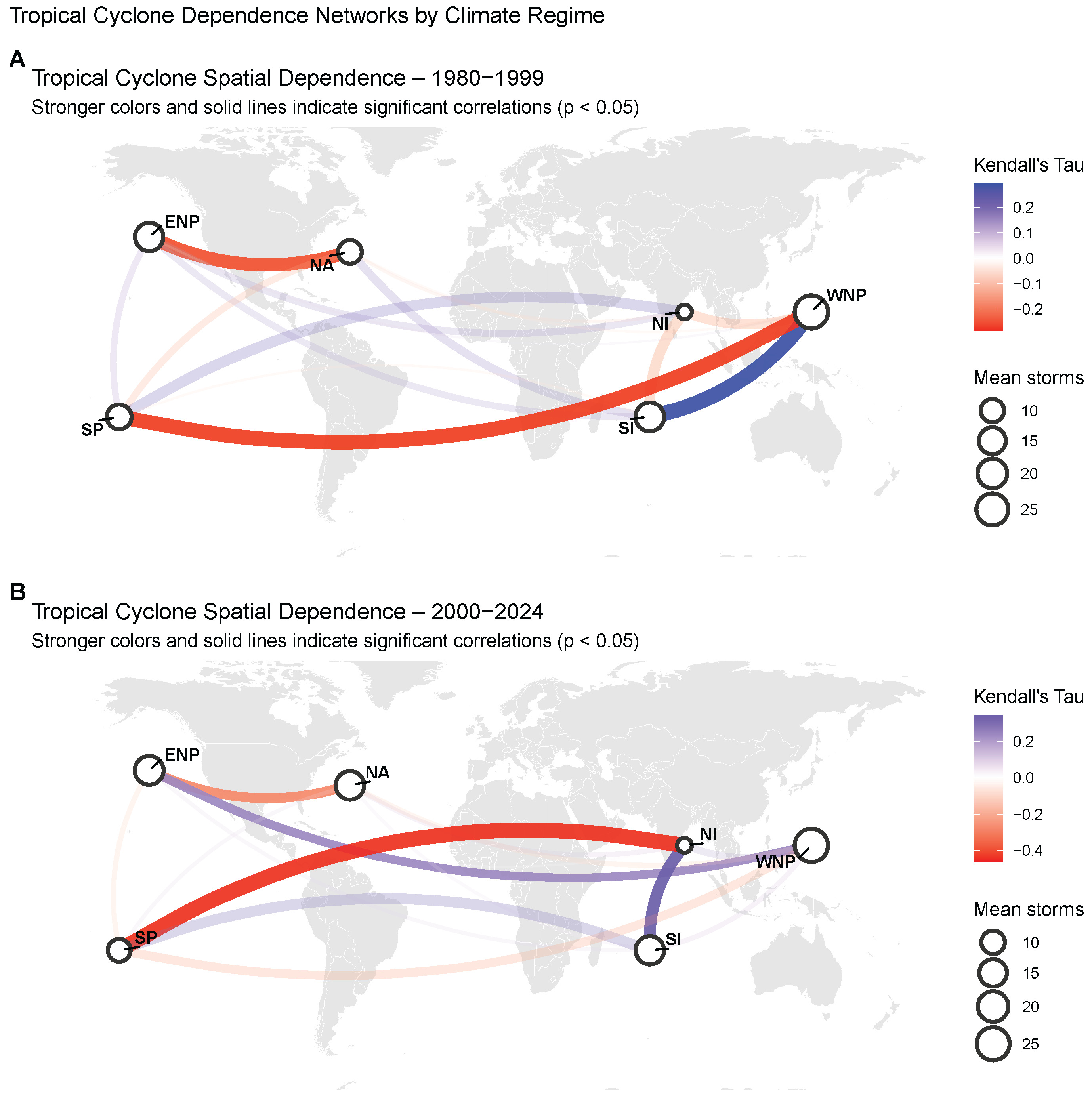
Figure 12 shows the global tropical cyclone basin dependence networks for 1980–1999 and 2000–2024, respectively, illustrating the enhanced connectivity and stronger dependence links in the recent regime. A comparative analysis of the two climate regimes reveals a distinct structural shift in the global tropical cyclone regional dependence network around the year 2000. During the first regime (1980–1999), significant dependencies represented by solid, deep-colored arcs in the network plot were primarily concentrated between the North Atlantic and East North Pacific (${\tau }_C=-0.257,p=0.011$) and within the Eastern Hemisphere between the Western North Pacific and both the Southern Indian (${\tau }_C=0.294,p=0.017$) and Southern Pacific (${\tau }_C=-0.283,p=0.014$) basins. In the second regime (2000–2024), while the negative ENP-NA relationship remained stable (${\tau }_C=-0.279$), the global coordination significantly reorganized: the Western North Pacific established a new significant positive correlation with the East North Pacific (${\tau }_C=0.238,p=0.014$), and the Northern Indian basin emerged as a dominant hub, developing strong significant dependencies with the Southern Indian (${\tau }_C=0.345,p=0.020$) and especially the Southern Pacific (${\tau }_C=-0.464,p<0.001$) basins. This transition from a WNP-centric dependency structure to a more globally interconnected network, characterized by the emergence of the Northern Indian basin as a critical node, underscores a fundamental change in the regional synchronization of global tropical cyclone activity following the structural break.

After splitting the record at the detected changepoint (year 2000), we obtain two distinct dependence structures. Using the copula-based Kendall’s tau estimates from Table 8, the matrices for the early regime (1980–1999) and the recent regime (2000–2024) are assembled below. The basins are ordered as before.

$${\mathbf{R}}_{\tau }^{\left(1\right)}=\begin{array}{cc}& \begin{array}{cccccc}\mathrm{ENP}& \mathrm{NA}& \mathrm{NI}& \mathrm{SI}& \mathrm{SP}& \mathrm{WNP}\end{array}\\ \begin{array}{c}\mathrm{ENP}\\ \mathrm{NA}\\ \mathrm{NI}\\ \mathrm{SI}\\ \mathrm{SP}\\ \mathrm{WNP}\end{array}& \left(\begin{array}{cccccc}1& -\mathbf{0}.\mathbf{257}& 0.138& 0.128& 0.126& 0.043\\ \begin{array}{c}\hfill -\mathbf{0}.\mathbf{257}\end{array}& 1& -0.063& 0.158& -0.133& -0.048\\ \begin{array}{c}\hfill 0.138\end{array}& -0.063& 1& -0.206& 0.209& -0.191\\ 0.128& 0.158& -0.206& 1& -0.047& \mathbf{0}.\mathbf{294}\\ \begin{array}{c}\hfill 0.126\end{array}& -0.133& \begin{array}{c}\hfill 0.209\end{array}& -0.047& 1& -\mathbf{0}.\mathbf{283}\\ 0.043& -0.048& -0.191& \mathbf{0}.\mathbf{294}& -\mathbf{0}.\mathbf{283}& 1\end{array}\right)\end{array}{\mathbf{R}}_{\tau }^{\left(2\right)}=\begin{array}{cc}& \begin{array}{cccccc}\mathrm{ENP}& \mathrm{NA}& \mathrm{NI}& \mathrm{SI}& \mathrm{SP}& \mathrm{WNP}\end{array}\\ \begin{array}{c}\mathrm{ENP}\\ \mathrm{NA}\\ \mathrm{NI}\\ \mathrm{SI}\\ \mathrm{SP}\\ \mathrm{WNP}\end{array}& \left(\begin{array}{cccccc}1& -\mathbf{0}.\mathbf{279}& -0.022& 0.080& -0.124& \mathbf{0}.\mathbf{238}\\ \begin{array}{c}\hfill -\mathbf{0}.\mathbf{279}\end{array}& 1& 0.116& 0.060& 0.078& -0.125\\ \begin{array}{c}\hfill -0.022\end{array}& 0.116& 1& \mathbf{0}.\mathbf{345}& -\mathbf{0}.\mathbf{464}& 0.187\\ 0.080& 0.060& \mathbf{0}.\mathbf{345}& 1& 0.312& 0.117\\ \begin{array}{c}\hfill -0.124\end{array}& 0.078& \begin{array}{c}\hfill -\mathbf{0}.\mathbf{464}\end{array}& 0.312& 1& -0.247\\ \mathbf{0}.\mathbf{238}& -0.125& \mathit{0}.\mathit{187}& 0.117& -0.247& 1\end{array}\right)\end{array}$$

(34)

Comparing the two matrices reveals a substantial shift. The average absolute off-diagonal entry increases from $0.15$ in the early regime to $0.19$ in the recent regime, indicating stronger overall coupling. Most strikingly, the Northern Indian basin, which had only weak connections in 1980–1999, becomes a central node in 2000–2024: it shows a strong positive dependence with the Southern Indian ($\tau =0.345$) and an even stronger negative dependence with the Southern Pacific ($\tau =-0.464$). Conversely, the previously significant positive link between the Southern Indian and Western North Pacific ($\tau =0.294$) weakens and becomes non-significant ($\tau =0.117$). These matrix summaries provide a concise visualization of the evolving teleconnections discussed in Section 5.

Figure 12 and Table 8 visually and numerically confirm the reorganization that the link between the Northern Indian and Southern Pacific basins transforms from a non-significant positive dependence in 1980–1999 (Gaussian, ${\tau }_C=0.209,p=0.066$) to a remarkably strong and highly significant negative dependence in 2000–2024 (Gaussian, ${\tau }_C=-0.464,p<0.001$). The analysis of the North Atlantic (NA) basin across climate regimes reveals that its most robust and persistent relationship is with the East North Pacific (ENP), characterized by a consistent significant negative dependency that remains stable before (${\tau }_C=-0.257,p=0.011$) and after (${\tau }_C=-0.279,p=0.013$) the structural break. Interestingly, while the NA-ENP connection is a dominant and unchanging feature in the regional dependence network, other NA relationships exhibit notable instability or “sign-flipping” after 2000. For instance, the dependency between the North Atlantic and Southern Pacific (SP) flips from a negative correlation (${\tau }_C=-0.133$) in the first regime to a positive one (${\tau }_C=0.078$) in the second, and a similar reversal occurs with the Northern Indian (NI) basin.

The values reported at Table 8 are from a single randomized-PIT realization. A $B_{\mathrm{MC}}=500$ averaging run reproduces every ${\widehat{\tau }}_C$ within $\pm 0.04$ and every modal copula family unchanged; across-replication standard deviations are ≤0.04 for all 15 pairs presented at Table A2 for robustness.

5. Discussion

The inclusion of changepoint detection significantly improves our understanding of tropical cyclone dependence structures by accounting for non-stationarity that would otherwise be obscured in a single-period analysis. By modeling pre- and post-2000 regimes separately, we capture important changes in inter-basin relationships that are not evident under a stationary assumption. For example, the stationary analysis suggested a weak, non-significant dependence between the Northern Indian and Southern Pacific basins (${\tau }_C=0.096,p=0.257$). In contrast, the regime-switching analysis, revealed a post-2000 shift toward a strong negative association (${\tau }_C=-0.464,p<0.001$), indicating that the stationary model masked a meaningful structural change. A similar regime-dependent change is observed between the Eastern North Pacific and Western North Pacific basins. While the association was weak and non-significant during pre-2000, it became significantly positive in the post-2000 regime (${\tau }_C=0.238,p=0.014$), indicating a strengthening of inter-basin dependence in the later regime. This demonstrates that the two-stage framework provides a useful methodological advancement for analyzing non-stationary multivariate climate data.

Table 14. Comparison of existing results with the improvements achieved by the two-stage framework.

Aspect/Phenomenon	Existing Results (Other Methods)	Improvements (Our Two-Stage Method)
North Atlantic activity shift	Identified a shift starting 1995 (by observational comparison); compared pre- and post-1995 averages [16].	Precise changepoint detection at 2000; quantifies a 59% increase in mean annual storm counts from 10.43 to 16.58.
NA–ENP “see-saw”	Inverse relationship suggested; Pearson correlation used; persistence not formally tested [40].	Confirmed as the only persistent teleconnection for NA across both regimes; stable $\tau \approx -0.27$ in both periods.
Northern Indian basin’s role	Focused on IOD intensification; no statistical identification of NI as a teleconnection hub [20].	NI becomes a central node post-2000: strong positive dependence with SI ($\tau =0.345$) and strong negative with SP ($\tau =-0.464$, $p<0.001$).
Global dependence structure	Copulas applied stationarily; single family assumed for the whole period [41].	Regime-specific selection: Gaussian prevalence drops (53% to 33%), Gumbel increases (7% to 20%), revealing increased systemic risk.
Spurious aggregate (NA–SP)	Stationary analysis showed significant negative dependence ($\tau =-0.202$, $p=0.014$), potentially misinterpreted as a stable link.	After 2000 split, relationship becomes non-significant (pre: $p=0.267$; post: $p=0.646$). Proves the link was a statistical artifact of non-stationarity.

corroborates established findings while also highlighting several potential new dependencies.

The identified structural break around 2000 aligns with documented shifts in global climate patterns, including changes in Atlantic Multidecadal Oscillation, Pacific Decadal Oscillation, and anthropogenic climate shift impacts. The strengthening of regional dependencies in the recent regime suggests enhanced global coordination of tropical cyclone activity, possibly due to intensified teleconnections under climate shift.

The emergence of a strong negative dependence between Southern Pacific and Northern Indian basins (${\tau }_C=-0.464$) is consistent with interactions between the Indian Ocean Dipole and El Niño-Southern Oscillation. We frame this as a hypothesis suggested by the regime-conditional dependence pattern, not as a direct implication of the fitted copulas, since neither the IOD nor ENSO indices are explicitly included as covariates in the present model. This finding has important implications for seasonal forecasting and climate risk assessment in these regions. A notable contrast emerges when comparing the North Atlantic results with and without the inclusion of a change point (CP) or structural break point. In the aggregate analysis (1980–2024) without considering regimes, the North Atlantic shows a significant negative dependency with the Southern Pacific (${\tau }_C=-0.202,p=0.014$). However, once the 2000 change point is included, this relationship becomes statistically insignificant in both the pre-2000 (${\tau }_C=-0.133,p_C=0.267$) and post-2000 (${\tau }_C=-0.078,p_C=0.646$) periods. This indicates that the significant NA-SP dependency observed in the overall data is consistent with a statistical artifact of the long-term combined dataset rather than a stable physical dependency. By contrast, the NA-ENP relationship remains significant regardless of CP inclusion, which is suggestive of it being the only truly persistent regional driver for North Atlantic storm count variability across different climate states. The persistent negative correlation is consistent with a “see-saw” effect, plausibly modulated by large-scale atmospheric patterns like the Pacific North American (PNA) pattern or the position of the jet stream. When conditions are favorable for strong vertical wind shear in the ENP (reducing their counts), they are often unfavorable in the NA (increasing counts), and vice-versa. The fact that this relationship remains strong through both regimes is suggestive of a fundamental, hard-wired feature of Northern Hemisphere atmospheric dynamics, unlike the more transient teleconnections involving other basins. A formal test of these climate-mode hypotheses would require a covariate-conditional copula model with AMO/PDO/ENSO/IOD indices entering the marginals and/or the dependence parameters; this is identified as the most natural extension of the present framework and is discussed in the Future Work section.

This change in coordination structure is reflected by the increased prevalence of the Gumbel copula (an asymmetric copula with upper-tail dependence). This is consistent with a higher likelihood of concurrent extreme cyclone seasons across different basins, which has potential implications for global insurance and risk aggregation. The shift towards Gumbel copulas (upper-tail dependence) in the recent regime means that the probability of multiple basins having extremely high cyclone seasons simultaneously has increased. For global reinsurance applications, a stationary model would plausibly underestimate the risk of a year where, for example, the Western North Pacific, North Atlantic, and Southern Indian all experience catastrophic seasons concurrently. This “tail coincidence” risk is precisely what this study captures and is a relevant consideration for systemic risk assessment in the insurance industry.

Our study has several limitations: (1) sample size constraints in regime-specific analyses, (2) assumption of Poisson distribution for storm counts, (3) focus on total storms rather than intensity measures, (4a) bivariate copula analysis applied pair-by-pair, so for a fully coherent multivariate dependence model with $d\ge 3$, a vine (C-vine, D-vine, or regular vine) copula construction [27,28] would be required and is identified as a planned next step, and (4b) use of a single changepoint rather than multiple changepoints or continuous evolution. We additionally acknowledge: (5) the Stage 1 detector treats the Gaussian-copula correlation $\mathbf{R}$ as common across regimes, so the segmentation is most precisely interpreted as an intensity-shift detector under a fixed Gaussian-copula dependence; (6) the randomized PIT introduces auxiliary uncertainty that we mitigate by averaging over $B_{\mathrm{MC}}=500$ replications but cannot eliminate; (7) goodness-of-fit p-values are computed on the same data as the family-selection step and are therefore reported in a descriptive (not size-controlled) sense; (8) the i.i.d.-within-regime assumption cannot be tested with full power at the regime lengths of 20–25 years. Also, simulation results (Table 5) show that at $n=20$, the probability of correctly identifying the true copula family is only 38–51%. Therefore, the reported shift in family prevalence (e.g., Gumbel increasing from 7% to 20%) is best interpreted as a descriptive signal of changing tail behavior, not a statistically confirmed change in dependence type.

Future research should explore time-varying copulas such as the Bayesian dynamic models for extremes proposed by [10] that could offer a more granular view of evolving dependencies, incorporate intensity measures, and extend the analysis to include more basins and longer time series. Additionally, investigating the physical mechanisms underlying the identified dependence patterns would enhance the scientific understanding of global tropical cyclone teleconnections. Three further extensions are particularly natural: (a) direct copula-targeted detection following [35,36,37], which would test changes in dependence intrinsically rather than inferring them from a regime split chosen by marginal-plus-stationary-$\mathbf{R}$ likelihood; (b) discrete-copula frameworks [24,25,26] that avoid the randomized PIT; and (c) covariate-conditional copula models in which AMO, PDO, ENSO, and IOD indices enter the marginals and/or the dependence parameters, which would convert the climate-mode interpretations of Section 5 into formally testable hypotheses.

6. Conclusions

This study provides a comprehensive analysis of regional dependence structures of tropical cyclone counts across six major ocean basins from 1980 to 2024. By integrating changepoint detection with copula modeling, we identify significant non-stationarity in both marginal distributions and dependence structures. In particular, we detect a significant structural break around the year 2000, dividing the data into two distinct climate regimes. Across these regimes, storm frequency and dependence patterns changed significantly (e.g., a shift towards stronger, more extreme-value-focused copulas like Gumbel), including substantial changes in marginal distributions, most notably a 59% increase in North Atlantic storm frequency. The results reveal an evolution of dependence structures from primarily symmetric and weak to more complex and stronger over the regimes. Moreover, the study shows an emergence of new teleconnection patterns, particularly a strong negative dependence between Southern Pacific and Northern Indian basins.

Overall, this proposed two-stage analytical framework provides a useful approach for analyzing non-stationary multivariate climate data. These non-stationary findings suggest that climate risk assessments based on long-term averages may be outdated. Therefore, our two-stage framework provides a more flexible and dynamic picture of global TC teleconnections, which can improve seasonal forecasting and inform adaptation strategies in a changing climate. Ultimately, this two-stage analytical framework provides an alternative understanding of the impact of a changing climate on global tropical cyclone activities through the interdependence of basins. We acknowledge that the two-stage detector identifies changepoints under a Gaussian-copula stationary-$\mathbf{R}$ working model, and that direct copula-targeted detectors [35,36,37], discrete-copula frameworks [24,25,26], and covariate-conditional copulas are natural and important next steps that would refine the inference reported here. Given the sample size constraints, the evolutionary patterns reported here, particularly the shifts in copula family prevalence and the emergence of specific negative dependencies, should be viewed as hypothesis-generating for future studies with longer time series and formal tests of copula stability.