The Stingray Copula for Negative Dependence

Abstract

We present a new single-parameter bivariate copula, called the Stingray, that is dedicated to representing negative dependence, and it nests the Independence copula. The Stingray copula is generated in a relatively novel way; it has a simple form and is always defined over the full support, unlike many copulas that model negative dependence. We provide visualizations of the copula, derive several dependence properties, and compute basic concordance measures. We compare it with other copulas and joint distributions with respect to the extent of dependence it can capture, and we find that the Stingray copula outperforms most of them while remaining competitive with well-known, widely used copulas such as the Gaussian and Frank copulas. Moreover, we show, through simulation, that the dependence structure it represents cannot be fully captured by these copulas, as it is asymmetric. We also show how the non-parametric Spearman’s rho measure of concordance can be used to formally test the hypothesis of statistical independence. As an illustration, we apply it to a financial data sample from the building construction sector in order to model the negative relationship between the level of capital employed and its gross rate of return.

1. Introduction and Motivation

Casually observing a negative relation between two factors in all strands of life is a trivial matter: an increase in sugar intake tends to decrease dental health; an increase in exercise tends to decrease body weight; when the temperature rises, the consumption of hot drinks tends to decrease, etc. But in these examples and others like them, there is a direct causal, and often physical, treatment effect of one factor on the other that tends to produce the negative relation. While, strictly speaking, the relation should be modeled as stochastic and not deterministic since other factors are expected to come into play, at the same time, it remains mostly a strong and almost-deterministic relation with random two-sided shocks.

More interesting are cases where a negative relation/dependence arises between two non-negative random variables in systems, socio-economic, or other, with “automatic stabilizers” in some equilibrium region, and where the movement of one variable towards one direction often triggers the movement of the other towards the opposite direction. The negative relation between selling price and quantity demanded in open markets is one economic example that comes easily to mind. Yet again, more complex frameworks that give rise to negative dependence are those in which an increase in one factor is associated with influences that lead to a decrease in the other. One such example, which we will develop in some detail in the empirical section of this study, is the negative dependence between the size of the capital base of a firm and the rate of return on capital.

Moreover, the existence of negative dependence, which speaks for the dominant underlying relation, does not preclude the occurrence of “positive relation” events. For example, while indeed selling prices tend to be negatively correlated with quantities sold, low prices-low quantities as well as high prices-high quantities are not impossible, or even very rare, events. Therefore, in addition to modeling what happens along the “negative dependence” axis, it is important to capture the characteristics of the relation along the positive dependence axis, which, although weaker and less frequent, also materializes. This more strongly introduces the possibility of asymmetries, and the Stingray copula that we present in this study can model asymmetries with respect to positive dependence. For example, consider the relationship between family poverty and educational achievement: the negative relationship between the two appears to be well documented. But what happens with the joint events of positive relation, “high poverty-high educational achievement”, $\left(HH\right)$, and also “low poverty-low educational achievement”, $\left(LL\right)$? One could plausibly argue that the $\left(HH\right)$ event may be more frequent than the $\left(LL\right)$ event because educational achievement can serve as an instrument for socioeconomic advancement. Ultimately, this is a matter of empirical investigation, but the prospect of asymmetry in the joint probabilistic structure is there, and it requires a tool capable of modeling such asymmetries.

Negative dependence has received rather less attention than positive dependence in the literature. To provide an informal metric on a natural experiment, the Karlin and Rinott [1] paper pertaining to positive dependence has exactly five times more citations in Google Scholar as of 16 December 2025, from its twin paper Karlin and Rinott [2] that examines topics related to negative dependence. Of course, negative dependence has been examined in certain detail. Apart from the general books on copulas included in the References, indicative literature includes Lehmann [3], Jogdeo and Patil [4], Ebrhaimi and Ghosh [5], Block, Savits, and Shaked [6], Joag-Dev and Proschan [7], Hu and Yang [8], Amini, Nili Sani, and Bozorgnia [9].

This is perhaps due to the fact that, for the bivariate case, as Drouet Mari and Kotz [10] (pp. 43–44) mention, the results for negative dependence are mostly a ‘minus’ sign, or a reversion of an inequality, away from the results for positive dependence. To put it in a more direct way, negative dependence between a variable U and a variable V is equivalent to positive dependence between U and $-V$.

While this is not disputable, the implied tactic for applied research is not really productive. This tactic would advise, “if you have negative dependence between two variables and you need to model it, multiply one of the two data series by $-1$, and use a copula that reflects positive dependence”. There are at least three reasons why this approach is problematic: first, it is not at all certain that this ‘sign-flip’ will not conflict somewhere with the computational environment and estimation strategy and code used by the applied researcher, for reasons that have to do with software languages and their computational conventions (or the coding habits of the researcher). And the more complex this environment is, the more time-consuming it will be to audit and adjust it to work smoothly with the sign-flipped data series. Second, we sometimes need to implement data transformations that cannot be applied to negative data; the logarithm is the obvious example. Third, even if we manage to overcome these hurdles, once we’re done with estimation, we will have to spend extra time translating the software output back into what actually holds, both to perform inference and to prepare it for presentation to whoever expects it.

Overall, the frequent occurrence of negative dependence, together with the aforementioned realities of applied research, makes the development of bivariate negative dependence structures worthwhile if our interest also lies in providing tools for empirical research.

The relative sparsity of statistical tools for negative dependence is also evident in the copula field. Inspecting Table 4.1 of Joe [11] (p. 161), only six out of the 29 copulas listed can represent negative dependence (amusingly, this is again a five-to-one ratio in favor of positive dependence, as was the case with the two Karlin and Rinott articles mentioned earlier.) Moreover, and apart from workhorses like the Gaussian and Frank copulas (to which we will return), in many if not all other cases, the achieved strength of negative dependence is low, or it reaches the theoretical extreme at the price of sacrificing a considerable part of the copula support.

A well-known example here is the benchmark bivariate “Clayton” copula, which sometimes appears in the literature under different names. Wrestling with Stigler’s law of eponymy, Joe [11] dutifully calls this copula “Mardia–Takahasi–Cook–Johnson” (MTCJ), writing (p. 170) “The abbreviation to MTCJ follows the abbreviation style of FGM used for Farlie–Gumbel–Morgenstern; the initial C can also include Clayton for the bivariate copula.” The Clayton copula mainly represents positive dependence. It can represent negative dependence also, if the range of its parameter is extended to include $[-1,0)$. In that case, while it can reach the extreme value $-1$ for Kendall’s $\tau$, it loses support. In order to have $\tau =-0.5$ it must shed $\approx 29.5\%$ of it, while at the extreme $\tau =-1$, only half of the support remains. As Joe [11] (p. 168) comments, due to this weakness, “the extension is not useful for statistical modeling.”

Analogous is the case in a recent proposal for a copula dedicated to modeling negative dependence by Ghosh, Bhuyan, and Finkelstein [12]. They manage to allow for the full negative range $[-1,0]$ of concordance measures like Kendall’s $\tau$, but their copula is a piece-wise function that early on excludes whole areas of the ${[0,1]}^2\equiv {\mathbf{I}}^2$ support as dependence becomes visible and increases (see their scatter plots in their Figure 3, p. 1336). To give two specific examples, for $\tau =-0.5$, their Copula is defined only on $75\%$ of the ${\mathbf{I}}^2$ area, while for $\tau =-0.9$ it is defined only in 55% of the ${\mathbf{I}}^2$ support area.

The one-parameter bivariate Stingray copula that we present here is also constructed to represent exclusively negative dependence. It is generated by a relatively novel mathematical device, where one of the arguments of the copula also appears as an exponent to the other (see the recent works by Chesneau [13,14,15,16], where this construction approach is labeled “variable-power”. “Stingray” is certainly more ambitious aesthetically.) Still, it remains simple and transparent. It does not reach the strongest degree of dependence, but it still goes beyond where other copulas stop and maintains full support throughout. The fact that it does not reflect the theoretically maximum degree of dependence does not compromise its usefulness for empirical work, especially in the social sciences, where very strong dependence is the exception and not the rule. Moreover, the Stingray copula is asymmetric with respect to the “positive correlation” joint events, as we will see.

The rest of the article unfolds as follows: in Section 2 we present the basic mathematical functions (copula, conditional copulas, and the copula density), and we provide visual input for an intuitive understanding of how dependence looks under the Stingray. We also provide some probabilistic intuition related to its mathematical form. In Section 3, we present some of the main negative dependence properties that characterize our copula. In Section 4, we first compute the three main concordance measures (Kendall’s tau, Blomqvist-beta, and Spearman’s rho), and then we compare the Stingray copula to other bivariate distributions and copulas that can model negative dependence, in terms of their reach. Section 5 contains a simulation study to showcase the individuality of the dependence reflected by the Stingray copula against two all-purpose copula juggernauts (Gaussian and Frank). In Section 6, we develop a simple specification/goodness-of-fit test, and in Section 7 we fit the Stingray copula to an economic data set, exploring the relation between capital and its rate of return. Section 8 concludes. Some mathematical calculations and proofs are collected in the Appendix A and Appendix B.

2. The Stingray Copula

We consider a copula representation $C(u,v)$ for the joint distribution of two random variables $(X,Y)$ with absolutely continuous distribution functions $F\left(x\right)\equiv u,G\left(y\right)\equiv v$, where u and v are realizations from Uniforms (0,1). The new copula we present is

$$\mathrm{Pr}(X\le x,Y\le y)=C(u,v)={\left(u^{1+v^{\delta }}{v}^{1+u^{\delta }}\right)}^{1/2},-1\le \delta \le 0.$$

(1)

This function is grounded and has the proper margins,

$$\begin{array}{c}\hfill C(0,0)=C(1,0)=C(0,1)=0,\\ \hfill C(1,v)=v,C(u,1)=u,C(1,1)=1.\end{array}$$

It is also 2-increasing (i.e it satisfies the rectangle inequality). When the copula density exists, this is equivalent to the copula density being non-negative (Joe [17]) (p. 12). This is the case here, given the restriction on the dependence parameter $\delta$.

The copula is obviously symmetric in its arguments (but that does not mean that the allocation of joint probabilities is symmetric over the unit square). As we show later, its partial second derivatives are both positive, so it is subharmonic. Moreover, for $\delta =0$ we get $C(u,v)=uv\equiv \Pi$, the Independence copula, which is the one focal copula that is attainable here. Nesting the Independence copula is important for empirical work because whether dependence exists in the first place is crucial, especially in quantitative research in the social sciences, where statistical results provide critical support for causal arguments.

The conditional copulas are as follows (see Appendix A.1):

$$\begin{array}{c}\hfill \mathrm{Pr}(Y\le y\mid X=x)=C(v\mid u)={\displaystyle \frac{\mathsf{\partial }C(u,v)}{\mathsf{\partial }u}}={\displaystyle \frac{C(u,v)}{2u}}\left(\delta u^{\delta }lnv+1+v^{\delta }\right),\end{array}$$

(2)

$$\begin{array}{c}\hfill \mathrm{Pr}(X\le x\mid Y=y)=C(u\mid v)={\displaystyle \frac{\mathsf{\partial }C(u,v)}{\mathsf{\partial }v}}={\displaystyle \frac{C(u,v)}{2v}}\left(\delta v^{\delta }lnu+1+u^{\delta }\right).\end{array}$$

(3)

These can be used to simulate $(u,v)$ series that follow the Stingray copula, by the conditional distribution method (Nelsen [18]) (p. 41). We will also use them in deriving various properties of our copula, and also, in the empirical illustration of the paper, in order to perform a goodness-of-fit test that begins with the Rosenblatt transform.

2.1. The Copula Density

The copula density is as follows (see Appendix A.2):

$$\begin{array}{cc}\hfill c(u,v)& ={\displaystyle \frac{{\mathsf{\partial }}^{2}C(u,v)}{\mathsf{\partial }v\mathsf{\partial }u}}\hfill \\ \hfill & ={\displaystyle \frac{C(u,v)}{4uv}}\left[\left(\delta v^{\delta }lnu+1+u^{\delta }\right)\left(\delta u^{\delta }lnv+1+v^{\delta }\right)+2\delta (u^{\delta }+v^{\delta })\right].\hfill \end{array}$$

(4)

One can verify by computation that the copula density is everywhere non-negative for $-1\le \delta \le 0$. Indicatively, we have

$$\begin{array}{cc}\hfill \underset{u\to 1}{lim}c(u,v)& ={\displaystyle \frac{1}{2}}[\delta lnv+(1+\delta )(1+v^{\delta })],\hfill \\ \hfill \underset{v\to 1}{lim}c(u,v)& ={\displaystyle \frac{1}{2}}[\delta lnu+(1+\delta )(1+u^{\delta })],\hfill \\ \hfill \underset{u,v\to 1}{lim}c(u,v)& =1+\delta ,\hfill \end{array}$$

and these limits are non-negative for $\delta \in [-1,0]$.

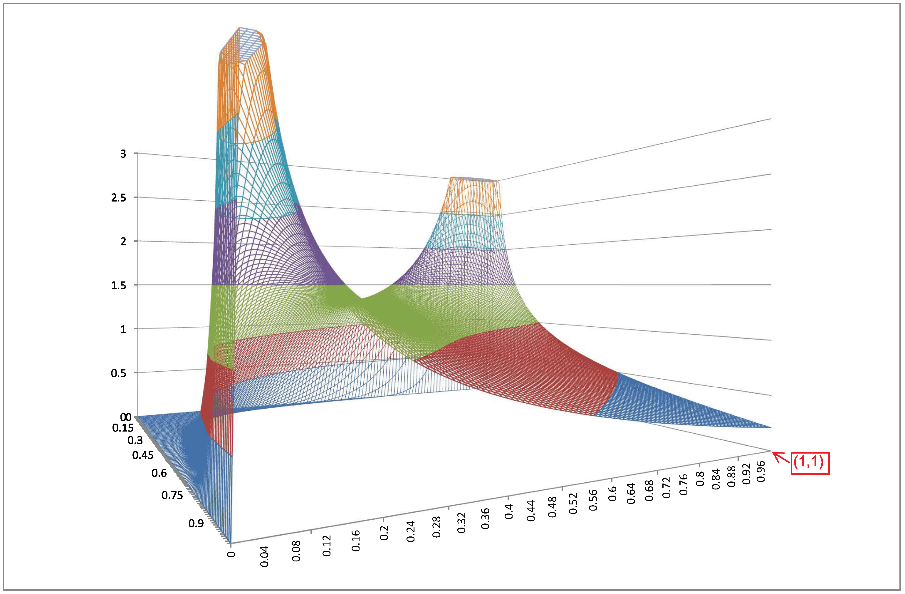
A 3-D image for this density is provided in Figure 1. The tip of the graph is at the $(1,1)$ point, and it touches zero for $\delta =-1$ (for $\delta =-1$, the Stingray copula coincides with the “variable-power 2” (VP2) copula presented in Chesneau [13], Proposition 4.2, p. 42, which, however stands alone since it does not incorporate a parameter that can vary in value).

2.2. Scatterplots and Negative Dependence

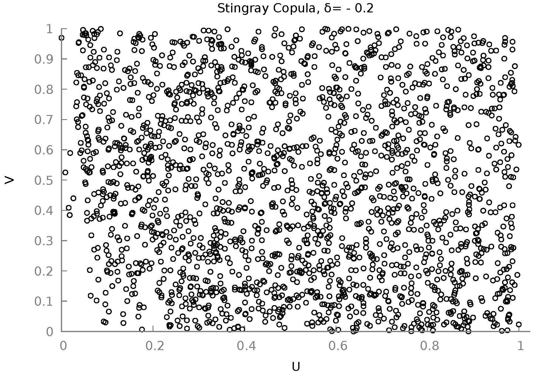
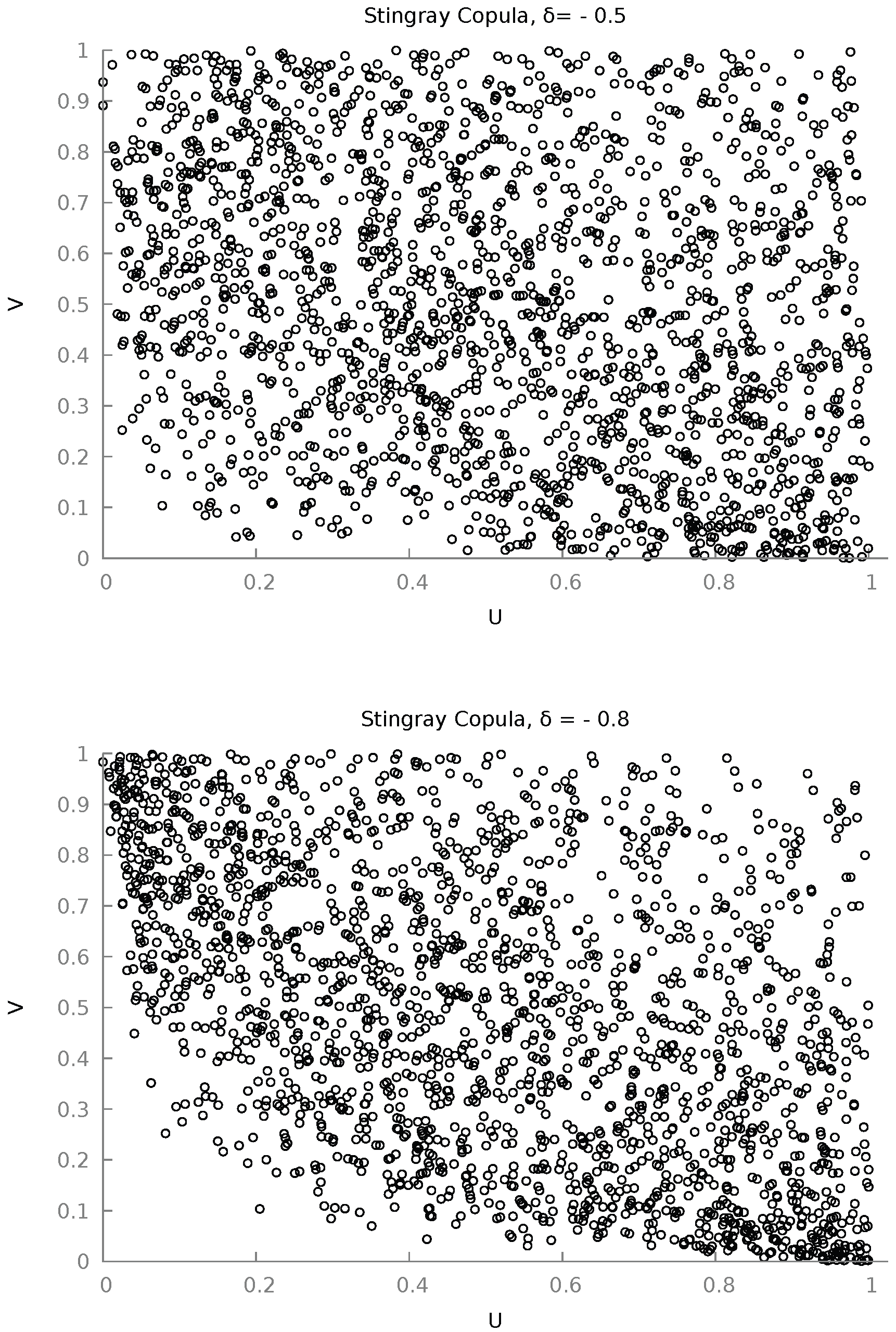
To obtain further visual intuition of the structure reflected by the Stingray copula we present in Figure 2 three scatter plots of $(u,v)$ for three gradually increasing values of $\delta$, using 2000 realizations.

The “convexity to the origin” that is clearly visible in the last scatter plot ($\delta =-0.8$) is observable in other copulas also. For example, Nelsen [18] (pp. 120–122) provides scatter plots of several Archimedean copulas, and among them there are five that exhibit this characteristic for some value of their parameter (they are, using the book’s numbering, 4.2.1, 4.2.2, 4.2.7, 4.2.15, 4.2.18). In fact, they have it much more sharply, and this is no accident; in all cases, these are copulas that use the $\max \{C,0\}$ device to keep the copula positive, and forcibly impose this no-probability land near the origin (and so for jointly low-probability events). As regards the direction of dependence, the scatter plots of Figure  also show that it is negative, as the copula density graph did previously. More formally we have (see Appendix A.3).

$${\displaystyle \frac{\mathsf{\partial }C(u,v;\delta )}{\mathsf{\partial }\delta }}>0.$$

(5)

Since $\delta \le 0$, this implies that as $\delta$ increases in absolute value, $C(u,v)$ decreases. The four fundamental underlying joint probability events for given $\left(F\right(x),G(y\left)\right)=(u,v)$ are as follows:

$$\mathrm{Pr}(X\le x,Y\le y)=C(u,v)\Rightarrow {\displaystyle \frac{\mathsf{\partial }}{\mathsf{\partial }\delta }}\mathrm{Pr}(X\le x,Y\le y)>0,$$

$$\mathrm{Pr}(X>x,Y>y)=1-u-v+C(u,v)\Rightarrow {\displaystyle \frac{\mathsf{\partial }}{\mathsf{\partial }\delta }}\mathrm{Pr}(X>x,Y>y)>0,$$

$$\mathrm{Pr}(X\le x,Y>y)=u-C(u,v)\Rightarrow {\displaystyle \frac{\mathsf{\partial }}{\mathsf{\partial }\delta }}\mathrm{Pr}(X\le x,Y>y)<0,$$

$$\mathrm{Pr}(X>x,Y\le y)=v-C(u,v)\Rightarrow {\displaystyle \frac{\mathsf{\partial }}{\mathsf{\partial }\delta }}\mathrm{Pr}(X>x,Y\le y)<0.$$

These relations formalize the result that as the negative $\delta$ moves towards its lower bound $-1$, it is the last two joint events, which represent negative dependence, that acquire higher probability. Visualizing the joint support on the plane as a unit square, as $\delta$ moves towards $-1$, the probability mass moves towards the upper left and lower right regions, deserting the upper right and lower left.

2.3. Some Probabilistic Intuition

We noted that the mathematical device of using one copula variable as an exponent of the other appears relatively novel. We next show how to link this to probabilities and, in a more intuitive way, explain why the Stingray copula represents negative dependence and why it is asymmetric at the two corners of the positive diagonal. We start by manipulating the copula as follows (using the fact that $\delta$ is negative):

$$C(u,v)={\left(u^{1+v^{\delta }}{v}^{1+u^{\delta }}\right)}^{1/2}=\mathrm{\Pi }·{\left(u^{{\displaystyle \frac{1-v^{\left|\delta \right|}}{v^{\left|\delta \right|}}}}·v^{{\displaystyle \frac{1-u^{\left|\delta \right|}}{u^{\left|\delta \right|}}}}\right)}^{1/2}$$

So the Stingray copula can be seen as adjusting the Independence copula by the factor to the right. We note that negative dependence implies that the fundamental joint probability of same-direction inequalities $\mathrm{Pr}(X\le x,Y\le y)$ is smaller than the probability under Independence, and the adjustment factor above is always smaller than unity. Hence, we get $C(u,v)\le \mathrm{\Pi }$, which is why the Stingray copula reflects negative dependence.

We turn now to the issue of asymmetry along the positive diagonal in the unit square. For clarity, let us examine the case where $\delta =-1$. We also have the following correspondences:

$$u=F\left(x\right)=\mathrm{Pr}(X\le x),v=G\left(y\right)=\mathrm{Pr}(Y\le y).$$

Then we can write, say, for the first component of the adjustment factor,

$$\delta =-1\Rightarrow u^{{\displaystyle \frac{1-v^{\left|\delta \right|}}{v^{\left|\delta \right|}}}}=u^{{\displaystyle \frac{1-v}{v}}}={\left[\mathrm{Pr}(X\le x)\right]}^{\left[\mathrm{Pr}\right(Y>y)/\mathrm{Pr}(Y\le y\left)\right]}.$$

If we examine a value for Y below its median $\mathrm{med}\left(Y\right)$, we have

$$y<\mathrm{med}\left(Y\right)\Rightarrow \mathrm{Pr}(Y>y)>\mathrm{Pr}(Y\le y),$$

and the exponent in the expression will be higher than unity, and it will reduce the value of this adjustment component,

$$y<\mathrm{med}\left(Y\right)\Rightarrow u^{{\displaystyle \frac{1-v}{v}}}<u=\mathrm{Pr}(X\le x).$$

When the Stingray copula evaluates “probabilistically low” intervals for Y, the corresponding marginal probability for X is lowered in value as a contributor to the adjustment factor, tending to strengthen the latter’s effect towards negative dependence. Now,

$${\displaystyle \frac{\mathsf{\partial }}{\mathsf{\partial }\left|\delta \right|}}\left({\displaystyle \frac{1-v^{\left|\delta \right|}}{v^{\left|\delta \right|}}}\right)>0,$$

meaning that as $\delta$ approaches zero from below, it weakens the effect of the exponent, operating as a regulator of the strength of the relation, on top of its inherent tendency towards negative dependence. The same analysis holds identically for the other component of the adjustment factor. Combining the two explains why there is no symmetry between what happens to the lower-left part compared to the upper-right part of the scatter plots shown earlier. If we look at events where the chosen $(x,y)>\left(\mathrm{med}\right(X),\mathrm{med}(Y\left)\right)$, both components of the adjustment factor will tend to increase their value, hence we will get more probability mass in the upper right quadrant than in the lower left quadrant. The overall adjustment factor is the geometric mean of the two and reflects both negative dependence and this asymmetry along the positive diagonal. Moreover, this analysis shows that one could explore an asymmetric version of the Stingray Copula, where only one of the two components of the adjustment factor is present, say,

$$K(u,v)=u{\left(v^{1+u^{\delta }}\right)}^{1/2}=\mathrm{\Pi }·{\left(v^{{\displaystyle \frac{1-u^{\left|\delta \right|}}{u^{\left|\delta \right|}}}}\right)}^{1/2}.$$

But we leave that for future research.

3. Negative Dependence Properties

In this section, we present some negative dependence properties of the Stingray copula. For the tail properties, we will also present natural extensions of the properties usually mentioned in the literature, now for the negative-dependence tails.

3.1. Quadrant Dependence

The Stingray copula is Negative Quadrant Dependent (NQD),

$$C(u,v)\le uv,\forall (u,v).$$

Under negative dependence, joint same-direction inequality events have everywhere a lower probability of occurring compared to the corresponding joint events under independence. This is an intuitive way to understand negative dependence. It also implies that for strictly increasing transformations $h_1,h_2$ of the underlying random variables $(X,Y)$, including the identity transformation, the covariance will be non-positive,

$$\mathrm{NQD}\Rightarrow \mathrm{Cov}(h_1\left(X\right),h_2\left(Y\right))\le 0.$$

3.2. Reverse Rule of Order 2

The Stingray copula is ${\mathrm{RR}}_2$ (“reverse rule of order 2”). Following Joe [17] (p. 23), we express this as

$$u_1\le u_2,v_1\le v_2,C(u_1,v_1)C(u_2,v_2)\le C(u_1,v_2)C(u_2,v_1).$$

The property can be proved by direct application of the definition (see Appendix B.1). Opportunity given, we note that Samuel Karlin has sown some confusion related to terminology as regards what the acronym RR corresponds to. In Karlin [19] (p. 12) he uses the abbreviation ‘SR’ for “sign-regularity” and then ‘RR’ writing “where the letters represent an abbreviation of the sign-reversal rule”. From this, it makes sense to translate ‘RR’ as “reverse-regular” (sign), and this is how Block, Savits, and Shaked [6] use it, and so do Joag-Dev and Proschan [7], Nelsen [20], Drouet Mari and Kotz [10], and Balakrishnan and Lai [21]. But in Karlin and Rinott [2] the authors clearly state ‘RR’ to mean “reverse rule”, and other authors like Joe [17] follow this translation. Nelsen [18] (p. 199) simply states both.

3.3. Concordance Ordering

Our copula is concordance-increasing (Joe [11]) (pp. 51–52) in the sense that

$${\delta }_1\le {\delta }_2\Rightarrow C(u,v;{\delta }_1)\le C(u,v;{\delta }_2),\forall (u,v).$$

This comes directly from the earlier result Equation (5), that the derivative of the Stingray copula with respect to $\delta$ is everywhere positive. If we examine a higher $\delta$, i.e., a $\delta$ closer to zero, we get less negative dependence and so more concordance. This aligns with the fact that for $\delta =0$ we get statistical independence.

3.4. Stochastic Monotonicity

The Stingray copula is stochastically decreasing (SD):

$$\begin{array}{c}\hfill {\displaystyle \frac{\mathsf{\partial }}{\mathsf{\partial }y}}\mathrm{Pr}(X>x\mid Y=y)=-{\displaystyle \frac{\mathsf{\partial }}{\mathsf{\partial }v}}C(u\mid v)<0,\forall u.\end{array}$$

(6)

$$\begin{array}{c}\hfill {\displaystyle \frac{\mathsf{\partial }}{\mathsf{\partial }x}}\mathrm{Pr}(Y>y\mid X=x)=-{\displaystyle \frac{\mathsf{\partial }}{\mathsf{\partial }u}}C(v\mid u)<0,\forall v.\end{array}$$

(7)

As we examine higher and higher y-values, the probability that X exceeds any given threshold is decreasing. The same holds for Y given $X=x$. This is essentially the “regression dependence” property of Lehmann [3], but using the complementary probability, which is more intuitive, linking an increasing derivative with positive dependence and a decreasing one with negative. The SD property implies, but is not implied by, negative quadrant dependence, but we stated NQD first due to its conceptual importance. We provide the proof of the SD property in the Appendix B.2, where we essentially show that the Stingray copula has positive second partial derivatives (which also makes it subharmonic).

3.5. Tail Monotonicity

Stochastic monotonicity implies also tail monotonicity, see Nelsen [18] (Th. 5.2.12, p. 197). For the case of negative dependence, this means that the Stingray copula is:

• Left-Tail Increasing (LTI):

  $${\displaystyle \frac{\mathsf{\partial }}{\mathsf{\partial }x}}\mathrm{Pr}(Y\le y\mid X\le x)={\displaystyle \frac{\mathsf{\partial }}{\mathsf{\partial }u}}\left({\displaystyle \frac{C(u,v)}{u}}\right)>0,\forall v.$$

  (8)

  This result, although certainly linked to negative dependence, does not provide an intuitive description that invokes it, and we will remedy this in a few lines below.
• Right Tail Decreasing (RTD):

  $${\displaystyle \frac{\mathsf{\partial }}{\mathsf{\partial }x}}\mathrm{Pr}(Y>y\mid X>x)=-{\displaystyle \frac{\mathsf{\partial }}{\mathsf{\partial }u}}\left({\displaystyle \frac{v-C(u,v)}{1-u}}\right)<0,\forall v.$$

  (9)

  Here we can say that as we increase x the probability that Y exceeds any given threshold decreases, which is a good way to think about negative dependence.

We get the same results if we switch places between X and Y.

In preparation for the four tail-dependence coefficients that we will examine immediately after (for a reason), we note that while for the concept of stochastic monotonicity the adjectives “left–right’ are used, for the concept of tail dependence the literature uses “lower-upper” instead, to refer to the same two tails of a univariate distribution. But the bivariate copula has four tails in the plane, and we are particularly interested in the two that are not depicted by the above probabilities. We want the probabilities where the conditioning event has an inequality of opposite direction, and thankfully, combining these two pairs of words, we can categorize transparently without confusion.

Keeping the unit square in mind and also the conventions that we linked X to u, and then we put u on the horizontal axis, we have that if the “left tail” is in reality the lower left one when we look at a bivariate copula, we can examine what happens to the (upper) left tail by

$$\left(\mathrm{upper}\right)\mathrm{Left}\mathrm{Tail}:{\displaystyle \frac{\mathsf{\partial }}{\mathsf{\partial }x}}\mathrm{Pr}(Y>y\mid X\le x)=-{\displaystyle \frac{\mathsf{\partial }}{\mathsf{\partial }u}}\left({\displaystyle \frac{C(u,v)}{u}}\right)<0,\mathrm{if}\mathrm{LTI}.$$

We see from Equation (8) that if the copula is “lower Left Tail Increasing”(LTI), it will necessarily be “upper Left Tail Decreasing”. Looking at the probability characterizing the upper left tail, we could describe this by saying that as we decrease x, the probability that Y exceeds any given threshold increases, and this is an intuitive description of negative dependence.

Also, if the “right tail” is the upper one, we can examine the lower right tail by the following:

$$\left(\mathrm{lower}\right)\mathrm{Right}\mathrm{Tail}:{\displaystyle \frac{\mathsf{\partial }}{\mathsf{\partial }x}}\mathrm{Pr}(Y\le y\mid X>x)={\displaystyle \frac{\mathsf{\partial }}{\mathsf{\partial }u}}\left({\displaystyle \frac{v-C(u,v)}{1-u}}\right)>0,\mathrm{if}\mathrm{RTD}.$$

Here, from Equation (9) we see that if the copula is “upper Right Tail Decreasing” (RTD), it will necessarily be “lower Right Tail increasing”. This can be translated as “when we increase the value x, the probability that Y is below any given threshold increases”, and this, again, is an intuitive description that pertains to negative dependence.

Table 1. Tail monotonicity in negative dependence.

Upper Left	⇓	⇓	Upper Right
Lower Left	⇑	⇑	Lower Right

summarizes these interrelations visually.

We close this section by examining tail dependence.

3.6. Tail Dependence

As in the previous section, we will examine four cases, in relation now to tail dependence, while usually only two are examined, the “upper” (meaning “upper right”), and the “lower” (meaning “lower left”), corresponding to the two corners along the positive dependence diagonal in the unit square. We will also examine the other two corners, those along the negative dependence diagonal. Here, the literature standard is to use L for “lower” (and not for “left”) and U for “upper”. We have the tail dependence coefficients:

$$\begin{array}{cccc}\hfill {\lambda }_L& =\underset{t\to 0}{lim}\mathrm{Pr}(v\le t\mid u\le t)\hfill & \hfill =& \underset{t\to 0}{lim}{\displaystyle \frac{C(t,t)}{t}},\hfill \\ \hfill {\lambda }_U& =\underset{t\to 1}{lim}\mathrm{Pr}(v>t\mid u>t)\hfill & \hfill =& \underset{t\to 1}{lim}{\displaystyle \frac{1-2t+C(t,t)}{1-t}},\hfill \\ \hfill {\lambda }_{U|left}& =\underset{t\to 0}{lim}\mathrm{Pr}(v>1-t\mid u\le t)\hfill & \hfill =& \underset{t\to 0}{lim}{\displaystyle \frac{t-C(t,1-t)}{t}},\hfill \\ \hfill {\lambda }_{L|right}& =\underset{t\to 0}{lim}\mathrm{Pr}(v\le t\mid u>1-t)\hfill & \hfill =& \underset{t\to 0}{lim}{\displaystyle \frac{t-C(1-t,t)}{t}}.\hfill \end{array}$$

We kept the standard notation ${\lambda }_L, {\lambda }_U$, and we made the other two fully transparent, sacrificing compactness. Due to the permutation symmetry of the copula, we have the following:

$${\lambda }_{U|left}={\lambda }_{L|right}.$$

The results for the Stingray copula are as follows:

$$\begin{array}{cc}\hfill \delta \in [-1,0],& {\lambda }_L={\lambda }_U=0,\hfill \end{array}$$

(10)

$$\begin{array}{ccc}\hfill \delta \in (-1,0],& {\lambda }_{U|left}={\lambda }_{L|right}=0,\hfill & \end{array}$$

(11)

$$\begin{array}{cc}\hfill \delta =-1,& {\lambda }_{U|left}={\lambda }_{L|right}=1-e^{-1/2}>0.\hfill \end{array}$$

(12)

We provide the calculations in Appendix B.3 and we have also verified them by computation. The Stingray copula does not, in general, exhibit “tail dependence” (joint events of extreme probabilities), except if it represents the maximum dependence allowable, in which case the negative dependence extreme events maintain at the limit a non-zero probability of occurring.

4. Negative Concordance Measures and Competitors

In this section, we first compute three basic concordance measures, Kendall’s $\tau$, Blomqvist-$\beta$ and Spearman’s ${\rho }_S$, and then we compare their maximum values (in absolute terms) with other copulas that can represent negative dependence, extending also the comparison in terms of Pearson’s correlation coefficient.

4.1. Kendall’s $\tau$

Kendall’s $\tau$ concordance coefficient can be expressed as follows:

$$\tau =4{\mathsf{\int }}_{{\mathbf{I}}^2}c(u,v)C(u,v)dudv-1.$$

We show in the Appendix B.4 that for the Stingray copula, we arrive at

$$\mathrm{Stingray}:\tau =\delta {\mathit{\int }}_{{\mathbf{I}}^2}{u}^{v^{\delta }}{v}^{u^{\delta }}(u^{\delta }+v^{\delta })dudv.$$

(13)

We computed this double definite integral for the deciles of $\delta$ using three different software. These were the integral2 function from the package pracma in the R platform, and the online calculators of Wolfram Alpha and of dcode.fr. They agreed, and its value is remarkably stable, very near $1/2$. We will provide these values later; for the moment, this implies that a good estimate for $\delta$ can be obtained by the sample estimate of Kendall’s $\tau$,

$$\widehat{\delta }=2\widehat{\tau }.$$

(14)

The maximum value in absolute terms of Kendall’s tau for the Stingray copula is $max\left|\tau \right|=0.511$. As Nelsen [20] shows, Kendall’s tau is also an average measure of the ${\mathrm{RR}}_2$ property.

4.2. Blomqvist-$\beta$ (Medial Correlation)

The Blomqvist-$\beta$ coefficient, often closely related to Kendall’s tau, is computed as follows:

$$\beta =4C(0.5,0.5)-1.$$

For the Stingray copula, we have the following:

$$\mathrm{Stingray}:\beta =2^{1-2^{-\delta }}-1.$$

(15)

Its maximum value in absolute terms is $max\left|\beta \right|=0.5.$

4.3. Spearman’s ${\rho }_S$

Spearman’s ${\rho }_S$ is computed as follows:

$${\rho }_S=12{\mathit{\int }}_{{\mathbf{I}}^2}C(u,v)dudv-3.$$

For the Stingray copula, its maximum value in absolute terms is $max|{\rho }_S|=0.693.$

While the value of this double integral changes as $\delta$ changes, there is a nearly linear relation between ${\rho }_S$ and $\delta$,

$$\mathrm{Stingray}:\delta \approx {\displaystyle \frac{{\rho }_S}{max|{\rho }_S|}}.$$

(16)

So, $\delta$ can be seen approximately as Spearman’s rho that holds in the data relative to the maximum ${\rho }_S$ value that the Stingray copula may acquire. In turn, Spearman’s rho is an average measure of quadrant dependence (see Nelsen [20]), and we will exploit this connection in the specification/goodness-of-fit test that we present later.

In

Table 2. Measures of concordance for the Stingray copula.

	Kendall’s Tau		Blomqvist	Spearman’s Rho
$\mathit{\delta }$	Integral	$\mathit{\tau }$	$\mathit{\beta }$	Integral	${\mathit{\rho }}_{\mathit{S}}$
−1	0.511283	−0.511	−0.5	0.192234	−0.693
−0.9	0.508973	−0.458	−0.451	0.197375	−0.632
−0.8	0.506891	−0.406	−0.402	0.202677	−0.568
−0.7	0.505061	−0.354	−0.351	0.208138	−0.502
−0.6	0.503504	−0.302	−0.301	0.213752	−0.435
−0.5	0.502237	−0.251	−0.25	0.219514	−0.366
−0.4	0.501268	−0.201	−0.199	0.225413	−0.295
−0.3	0.500595	−0.15	−0.148	0.231433	−0.223
−0.2	0.500197	−0.1	−0.098	0.237557	−0.149
−0.1	0.500028	−0.05	−0.049	0.243758	−0.075
0	0.5	0	0	0.25	0

, we present the related detailed values.

From Table 2 we see how closely Blomqvist-$\beta$ is to Kendall’s tau for all values of $\delta$. We also note that the Kendall’s tau value of $-0.511$ means that there is ≈75.5% chance that the two random variables will move in opposite directions.

4.4. Judgment Day

How does the Stingray copula fare against other bivariate distributions and copulas that can represent negative dependence?

We begin by introducing Pearson’s “linear” correlation coefficient $\rho$, which has not yet been addressed. This measure of dependence is not margin-free, which may reduce its importance as a core feature of a copula. To the theorist. Because the applied researcher will almost always compute it and think about what it reveals. This is the same applied researcher who previously wanted to keep their data on the positive axis, and the negative linear correlation between two non-negative random variables is constrained. Moran [22] showed that for such a pair, Pearson’s $\rho$ cannot reach the value $-1$. Intuitively, this is due to the asymmetry in the support: One variable is free to go to infinity, while the other cannot go below zero. Moreover, the lowest possible value for $\rho$ is determined by the marginal distributions (while the properties of their joint distribution may shrink this value even closer to zero). For the case of two Exponential variates, this lowest possible value is $1-{\pi }^2/6\approx -0.645$. Papadopoulos et al. [23] compute the same bound for two Half-Normal random variables as ≈−0.857.

An example of further restriction due to the joint distribution is Gumbel [24], who presents a bivariate distribution with Exponential margins and with only negative dependence, where $-0.40365\le \rho \le 0$. Another example is the bivariate Exponential Extension of Freund [25] that stops at $\rho \ge -1/3$ (the margins here are mixtures of Exponentials). Papadopoulos et al. [23] have examined a bivariate Truncated Normal that has Truncated Skew Normal margins, whose correlation coefficient cannot go below $-0.217$. In comparison, we present in

Table 3. Estimated maximum Pearson’s $\rho$ under the Stingray copula and various margins.

	HN	Exp	GE	N	L
HN	−0.5918	−0.5304	−0.5638	−0.6698	−0.6648
Exp		−0.4632	−0.5043	−0.6272	−0.6361
GE			−0.5352	−0.6497	−0.6538
N				−0.6951	−0.6398
L					−0.6819

estimated correlation coefficients between variables that obey pairwise the Stingray copula, and have various margins, namely, Half-Normal (HN), Exponential (Exp), Generalized Exponential (GE, see Papadopoulos et al. [26]), but also of two-sided variables following the Normal (N) and the Laplace (L), in identical pairs but also in-between them (based on 10,000 bivariate Stingray draws with $\delta =-1$).

From Table 3 we obtain evidence that compared to the aforementioned bivariate distributions, the Stingray copula does better, in terms of Pearson’s $\rho$, in the sense of allowing for stronger negative linear dependence.

We turn now to copulas proper. We have already discussed in Section 1 the MTCJ (“Clayton”) copula and another newly proposed copula that exceeds the capabilities of the Stingray but at the expense of seriously restricted support. Regarding now other well-known copulas that can model negative dependence without losing support, the Farlie–Gumbel–Morgenstern does not go below $\tau =-2/9\approx -0.222$, $\beta =-0.25$, and ${\rho }_S=-1/3$, while the Ali–Mikhail–Haq copula can go down to $\tau =-0.1817$ and $\beta =-0.25$, but not more (for the latter see Genest and MacKay [27] for a simple computational formula). Chesneau [28] recently developed a two-parameter modification of the MTCJ copula. This copula maintains its full support when it represents negative dependence, but it has $\tau \ge -0.356$, $\beta \ge -0.377$. The Stingray copula has $\tau \ge -0.511$, $\beta \ge -0.5$, and ${\rho }_S\ge -0.693$, and hence has a higher reach in terms of all three concordance measures compared to these three copulas.

But we still have to face the big players in the room, and we have specifically in mind the Gaussian, Student’s-t, the Plackett, and the Frank copulas, which are very popular and allow for full negative dependence in terms of concordance measures.

As regards the Gaussian copula, we find that in order to reflect negative dependence higher than the Stingray in terms of Kendall’s tau, Blomqvist’s $\beta$, or Spearman’s rho, it must be the case that its parameter $\rho$ falls below $-0.71$ (the Student’s-t copula has the same expression for $\tau$ as the Gaussian, so the same conclusion holds for it). As regards the Plackett copula, which can represent negative dependence when its parameter $\theta$ is in $(0,1)$, we find that, related to Spearman’s rho, we must have $\theta \le 0.08$ to go beyond what the Stingray copula can represent, while as regards Blomqvist-$\beta$, we must have $\theta \le 0.11$. These copulas are comparable to the Stingray copula in the sense that their dependence parameter has a restricted support. We see that they surpass the Stingray’s capabilities only after exhausting a large portion of it, which allows us to argue that the Stingray is competitive here as well. However, the Frank copula has an unrestricted dependence parameter; therefore, in the next section, we provide an alternative comparison.

5. Individuality of the Stingray Copula: Simulation Study

In this section, we present a simulation study to show that the negative dependence represented by the Stingray copula is decisively distinct from that represented by the Gaussian and Frank copulas.

We generated draws from the Stingray copula, for $\delta =-0.5,-0.7,-0.9$ (so for Kendall’s $\tau \approx -0.25,-0.35,-0.45$), and for sample sizes $n=$ 100, 200, 500, so nine worlds in total. In each world, we performed 1000 repetitions, and in each repetition, we executed the likelihood test of Vuong [29] for non-nested likelihoods, between the Stingray and the Gaussian, and between the Stingray and the Frank copulas. This is a test whose null hypothesis is that the two contestant specifications are observationally equivalent, and the test is either inconclusive or it favors one of the two. In each of

Table 4. Specification tests, Stingray (S) vs Gaussian (G). Generated data is Stingray.

Sign of the likelihood test statistic
	$\delta =$	$-0.5$		$-0.7$		$-0.9$
		S > G	S < G	S > G	S < G	S > G	S < G
n	100	0.893	0.107	0.947	0.053	0.952	0.048
	200	0.949	0.051	0.991	0.009	0.99	0.01
	500	0.996	0.004	1	0	1	0
Rejection of ${\mathrm{H}}_0$ (distributional equivalence) with 90% confidence.
	$\delta =$	$-0.5$		$-0.7$		$-0.9$
		S > G	S < G	S > G	S < G	S > G	S < G
n	100	0.398	0.002	0.543	0.001	0.579	0.002
	200	0.551	0.001	0.746	0	0.804	0.002
	500	0.845	0	0.977	0	0.985	0

and

Table 5. Specification tests, Stingray (S) vs Frank (F). Generated data is Stingray.

Sign of the likelihood test statistic
	$\delta =$	$-0.5$		$-0.7$		$-0.9$
		S > F	S < F	S > F	S < F	S > F	S < F
n	100	0.927	0.073	0.969	0.031	0.978	0.022
	200	0.965	0.035	0.996	0.004	0.999	0.001
	500	0.999	0.001	1	0	1	0
Rejection of ${\mathrm{H}}_0$ (distributional equivalence) with 90% confidence.
	$\delta =$	$-0.5$		$-0.7$		$-0.9$
		S > F	S < F	S > F	S < F	S > F	S < F
n	100	0.416	0.003	0.658	0	0.747	0
	200	0.627	0.001	0.858	0	0.953	0
	500	0.9	0	0.991	0	0.998	0

, we report the proportion of times the test statistic favored mathematically the Stingray (and vice versa), and also the proportion of times the test statistic formally designated the Stingray copula as a better fit for the data (and vice versa), with 90% statistical confidence. In the Tables, S represents the Stingray, G the Gaussian, and F the Frank copula.

It is clear from the Tables that even with a small sample of $n=100$ and rather low dependence $\delta =-0.5$, the Vuong test almost all of the times detects that the Stingray is a better fit for the data (upper parts of the two Tables), although it needs a sample of $n=500$ to decisively declare it the winner, in more than 80% of the times (lower parts of the Tables). When dependence strengthens to $\delta =-0.7$ (Kendall’s $\tau \approx -0.35$), only 200 observations are needed to conclude that. This shows that, regardless of the flexibility of the Gaussian and Frank copulas, the dependence structure captured by the Stingray copula is distinctive, warranting its own distinct model. The fact that both the Gaussian and the Frank copulas are symmetric with respect to the allocation of joint probability mass in the unit square, whereas the Stingray copula can reflect asymmetries in that respect, is one of the main distinguishing factors here.

6. Specification Testing Under Quadrant Dependence

There are many specification/goodness-of-fit tests that have been developed for copulas (see e.g., Genest, Rémillard, and Beaudoin [30] for review and comparisons). Here, we devise a specification test that exploits the property of quadrant dependence and is simple to implement. The first step is to transform the specification test into a test of independence using the Rosenblatt transform, as originally presented in Rosenblatt [31]. Then we use the fact that under quadrant dependence (positive or negative), Spearman’s rho, besides being a measure of concordance, also becomes a measure of dependence, measuring the distance of the copula from the Independence one, and representing Independence if and only if it is zero. The property of quadrant dependence is essential because, in general, zero concordance does not imply independence.

In the bivariate case, testing the goodness-of-fit of a Copula specification through Rosenblatt’s transform amounts to testing for independence each of the following two bivariate vectors separately:

$$\left(u,C(v\mid u)\right)\stackrel{{\mathrm{H}}_0}{\sim }\mathrm{\Pi },\left(v,C(u\mid v)\right)\stackrel{{\mathrm{H}}_0}{\sim }\mathrm{\Pi }.$$

At the same time, when negative quadrant dependence exists as a property, a proper measure of dependence, Schweizer and Wolff’s $\sigma$ (see Nelsen [18]) (p. 209), is equal to the negative of Spearman’s rho:

$$\mathrm{NQD}\Rightarrow {\sigma }_{SW}=-{\rho }_S.$$

Since the asymptotic distribution of ${\widehat{\rho }}_S$ under the null Hypothesis is zero-mean Normal, the opposite sign does not affect the conclusion of the statistical tests. So we can test, as usual, the hypothesis that ${\rho }_S$ is statistically zero, between the two pairs of vectors separately that reflect Rosenblatt’s transform (these results hold, of course, also for positive quadrant dependence with the obvious sign adjustment.)

If this independence hypothesis holds, then the data follow the prescribed copula, as a theoretical certainty for the populations involved. In the real world, where things are never exact and standard errors undermine sharpness, if we fail to reject the null hypothesis of independence, at the very least, we can conclude that the specified copula performs well with the data.

7. An Empirical Illustration

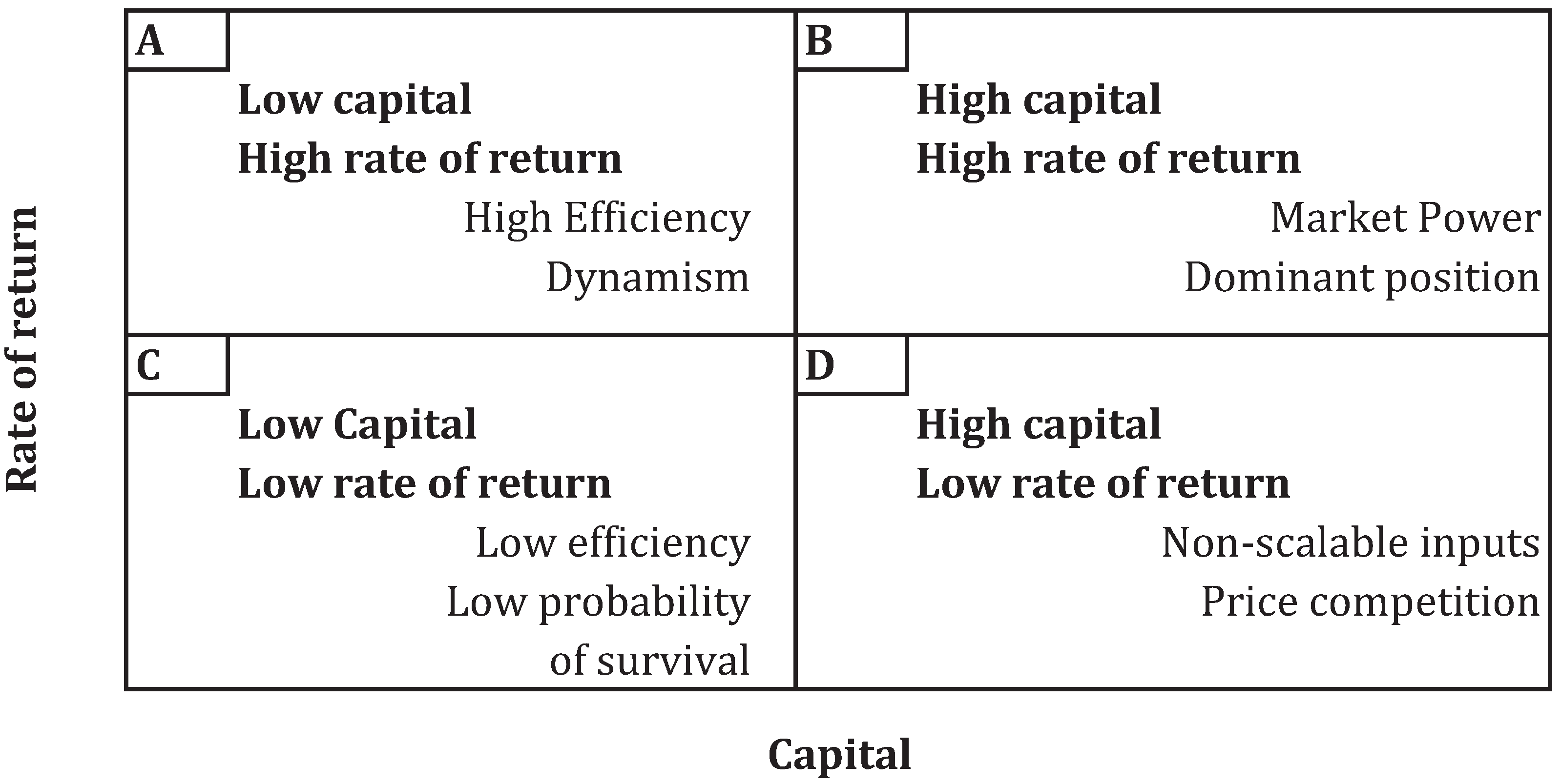
Among business persons and economists alike, there is, broadly speaking, an anticipation that the gross rate of return of capital tends to be negatively associated with the level of capital employed. Let X represent capital and W its returns, so $Y=W/X$ is the rate of return. We expect that W increases with X, but if it increases by less in proportional terms, then X and Y will be negatively correlated. Moreover, the relationship is expected to be asymmetric along the positive correlation axis, with higher frequency in the “high-high” (upper right) quadrant compared to the lower left quadrant. We summarize the situation in Figure 3.

The negative relation is expected to appear, first because as a firm expands its operations (high capital), it may encounter non-scalable or semi-scalable inputs which will bring about decreasing returns to scale, but also it will trigger antagonistic competition forces that may force the firm to offer lower prices than before, and hence lower returns although not lower capital (this is quadrant D of Figure 3). At the same time, the “low capital-high returns” event (quadrant A) refers to smaller firms that are highly efficient and remain in the market due to their positive economic performance and dynamism. And these are indeed the most common situations we encounter in open markets. As regards the positive dependence diagonal axis, the event “high capital-high returns” (quadrant B) is also observed when we have strong market power and domination that allows the firms to extract economic rents and thus higher returns, while the case of “low capital-low returns” (quadrant C) is relatively less likely, since in a more or less well-functioning market such firms have low probability of survival, leading to them being the smallest subset of firms.

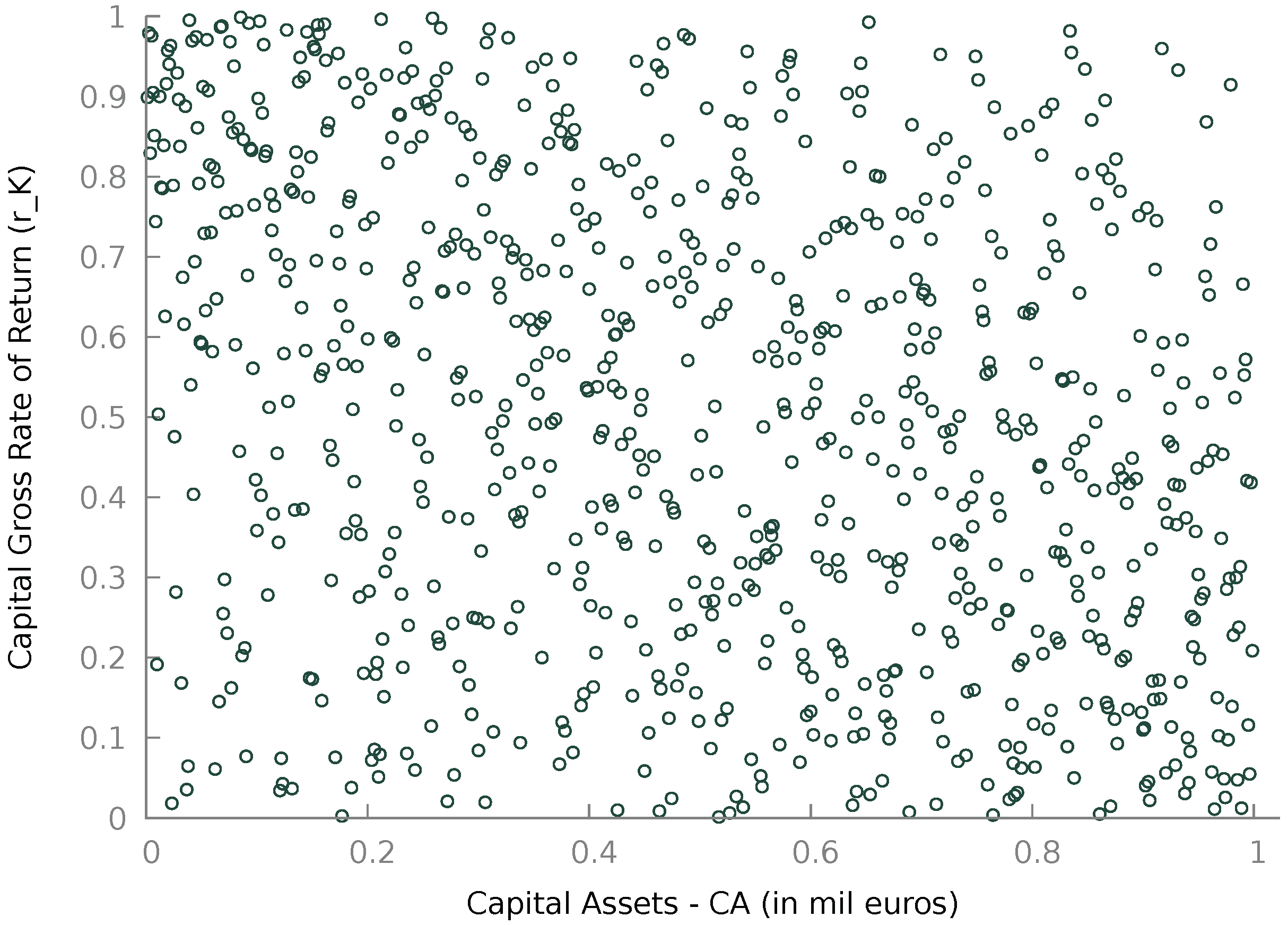
In this context, we examine a cross-sectional sample of $n=819$ Greek firms in the Buildings Construction sector (the 3-digit NACE rev2 classification is “412-Construction of residential and non-residential buildings”). The sample uses 2019 balance sheet data. We measure Capital Assets (CA) in the balance sheet as the sum of Fixed Assets and Inventory. As a measure of capital returns, we take the EBITDA (Earnings Before Interest, Taxes, Depreciation, and Amortization), which is standard international practice. Its ratio to the Capital Assets is the (gross) rate of capital returns ($r_K=\mathrm{EBITDA}/\mathrm{CA}$). We then compute the empirical distribution function of these two variables, CA and $r_K$, using for each

$${\widehat{F}}_Z\left(t\right)={\displaystyle \frac{1}{n+1}}\sum _{i=1}^{n}I(z_i\le t),Z=\mathrm{CA},r_K.$$

In Figure 4, we present the scatter plot of the empirical distribution functions of CA and $r_K$.

A cursory look may create the impression that there is no statistical dependence worthy of discussion in Figure 4. But Pearson’s correlation coefficient (among the original variables) was estimated as $\widehat{\rho }=-0.230$, Spearman’s rho as ${\widehat{\rho }}_S=-0.312$, and Kendall’s tau as $\widehat{\tau }=-0.213$. Not strong, but not negligible, and statistically non-zero. A calmer look at the scatter plot reveals the mild concentration of points along the negative diagonal, while enough points are found in the upper-right and lower-left regions. This is exactly the territory of the Stingray copula, where the real world ranges over the entire unit square but exhibits some negative association without being too vocal about it.

We now implement the specification test presented in the previous section. Namely, we will test, through Spearman’s rho, the null of independence between $\left(u,C(v\mid u)\right)$ and separately between $\left(v,C(u\mid v)\right)$, where the conditional copulas are Stingray. If independence is rejected, the Stingray should be rejected as an appropriate model for these data. If independence is not rejected, the Stingray copula can be considered an adequate model for this data set.

We make the test more strict by testing in parallel for a zero Kendall’s tau (which also follows asymptotically a zero-mean Normal under the null hypothesis). This creates four possible outcomes: $\{{\rho }_S\ne 0,\tau \ne 0\}$, $\{{\rho }_S\ne 0,\tau =0\}$, $\{{\rho }_S=0,\tau \ne 0\}$, $\{{\rho }_S=\tau =0\}$. Of these four, the first three lead to rejection of the null hypothesis and the Stingray specification. This is because the third possible outcome, $\{{\rho }_S=0,\tau \ne 0\}$, even though it has ${\rho }_S=0$, it is accompanied by the contradictory result $\tau \ne 0$. It is contradictory because under quadrant dependence ${\rho }_S$ is a measure of dependence while $\tau$ is still only a measure of concordance. And we cannot have zero dependence and non-zero concordance, hence this result is a sign of general misspecification. Only $\{{\rho }_S=\tau =0\}$ permits us to defend the specification under examination.

We computed $C(v\mid u)$ and $C(u\mid v)$ using the Stingray copula with $\widehat{\delta }=2\widehat{\tau }=-0.4258$, we estimated non-parametrically their ${\rho }_S$ and $\tau$ with u and v, respectively, and we tested for zero Spearman’s rho and zero Kendall’s tau following Genest and Favre [32]. The results are presented in

Table 6. Goodness of a fit test for the Stingray copula, $n=819$.

Test	(u, C(v∣u))	(v, C(u∣v))
${\widehat{\rho }}_S$	−0.0207	−0.0071
std. error	0.0349	0.0349
p-value	0.553	0.839
$\widehat{\tau }$	−0.0149	−0.0086
std. error	0.0233	0.0233
p-value	0.523	0.712

.

From Table 6, we see that the estimated sample concordance/dependence measures are already very small, and even though the large sample size leads to a low standard error of each statistic, the p-value of the test is very high in all four cases. Therefore, we conclude that both measures are zero, so the necessary and sufficient condition for the Rosenblatt transform cannot be rejected, and the Stingray copula can be considered an adequate modeling device for the specific data set.

8. Conclusions and Further Research

We have presented a new single-parameter bivariate copula, baptized the Stingray copula, that specializes in representing negative dependence. It has stochastic and tail monotonicity (for negative dependence), is concordance-increasing, satisfies the Reverse Rule of order 2, and is negative quadrant dependent. It can accommodate stronger dependence than comparable existing copulas, as measured by concordance measures such as Kendall’s tau and Spearman’s rho, without losing any part of the ${\mathbf{I}}^2$ support. It performs competitively with benchmark flexible all-purpose copulas like the Gaussian and the Frank, and it reflects a negative dependence structure that is not similar to what these copulas can model, since it reflects asymmetry along the positive dependence axis. It also outperforms bivariate distributions in terms of Pearson’s $\rho$ for various non-negative and two-sided margins. These results make it a potentially useful tool for statistical empirical work.

On the theoretical front, there appear to be at least five possible avenues for future research: the first is to increase the number of its parameters to extend its reach, but this must be balanced against the unavoidable complexity it may create in handling and estimation. The second question is whether it can be extended to accommodate more than two variables. The third is the development of the survival function and the Stingray survival copula, but based on the logic of negative dependence, namely for events $\{X>x,Y<y\}$ and vice versa. In addition, developing the Stingray Copula for count/discrete data would be fruitful, since many real-world phenomena are measured in this way, and Copulas of discrete data present their own peculiarities and challenges. Finally, the Stingray copula generates dependence by making one variable operate as an exponent of the other, a construction that has only recently emerged as a copula construction method. We provided some probabilistic intuition for how this works, and it is a method that can certainly be explored further for constructing copulas.

References

1. Karlin, S.; Rinott, Y. Classes of orderings of measures and related correlation inequalities. I. Multivariate totally positive distributions. J. Multivar. Anal. 1980, 10, 467–498. [Google Scholar] [CrossRef] [Scilit]
2. Karlin, S.; Rinott, Y. Classes of orderings of measures and related correlation inequalities II. Multivariate reverse rule distributions. J. Multivar. Anal. 1980, 10, 499–516. [Google Scholar] [CrossRef] [Scilit]
3. Lehmann, E.L. Some concepts of dependence. Ann. Math. Stat. 1966, 37, 1137–1153. [Google Scholar] [CrossRef] [Scilit]
4. Jogdeo, K.; Patil, G. Probability inequalities for certain multivariate discrete distribution. Sankhyā Indian J. Stat. Ser. B 1975, 37, 158–164. [Google Scholar]
5. Ebrahimi, N.; Ghosh, M. Multivariate negative dependence. Commun. Stat.-Theory Methods 1981, 10, 307–337. [Google Scholar] [CrossRef] [Scilit]
6. Block, H.W.; Savits, T.H.; Shaked, M. Some concepts of negative dependence. Ann. Probab. 1982, 10, 765–772. [Google Scholar] [CrossRef] [Scilit]
7. Joag-Dev, K.; Proschan, F. Negative association of random variables with applications. Ann. Stat. 1983, 11, 286–295. [Google Scholar] [CrossRef] [Scilit]
8. Hu, T.; Yang, J. Further developments on sufficient conditions for negative dependence of random variables. Stat. Probab. Lett. 2004, 66, 369–381. [Google Scholar] [CrossRef] [Scilit]
9. Amini, M.; Nili Sani, H.; Bozorgnia, A. Aspects of negative dependence structures. Commun. Stat.-Theory Methods 2013, 42, 907–917. [Google Scholar] [CrossRef] [Scilit]
10. Drouet Mari, D.; Kotz, S. Correlation and Dependence; Imperial College Press: London, UK, 2001. [Google Scholar]
11. Joe, H. Dependence Modelling with Copulas; CRC Press: Boca Raton, FL, USA, 2015. [Google Scholar]
12. Ghosh, S.; Bhuyan, P.; Finkelstein, M. On a bivariate copula for modeling negative dependence: Application to New York air quality data. Stat. Methods Appl. 2022, 31, 1329–1353. [Google Scholar] [CrossRef] [Scilit]
13. Chesneau, C. Theoretical validation of new two-dimensional one-variable-power copulas. Axioms 2023, 12, 392. [Google Scholar] [CrossRef] [Scilit]
14. Chesneau, C. Some new developments on variable-power copulas. Appl. Math. 2023, 50, 35–54. [Google Scholar] [CrossRef] [Scilit]
15. Chesneau, C. Investigation of a variable-power FGM-type copula. Stoch. Model. Probab. Stat. 2024, 1, 17–36. [Google Scholar]
16. Chesneau, C. Solutions to two open problems on bivariate variable-power copulas. Bull. Comput. Appl. Math. 2024, 12, 93–118. [Google Scholar]
17. Joe, H. Multivariate Models and Multivariate Dependence Concepts; CRC Press: Boca Raton, FL, USA, 1997. [Google Scholar]
18. Nelsen, R. An Introduction to Copulas, 2nd ed.; Springer Science & Business Media: New York, NY, USA, 2006. [Google Scholar]
19. Karlin, S. Total Positivity; Standford University Press: Stanford, CA, USA, 1968; Volume 1. [Google Scholar]
20. Nelsen, R.B. On measures of association as measures of positive dependence. Stat. Probab. Lett. 1992, 14, 269–274. [Google Scholar] [CrossRef] [Scilit]
21. Balakrishnan, N.; Lai, C.D. Continuous Bivariate Distributions, 2nd ed.; Springer: Berlin/Heidelberg, Germany, 2009. [Google Scholar]
22. Moran, P.A.P. Testing for correlation between non-negative variates. Biometrika 1967, 54, 385–394. [Google Scholar] [CrossRef] [Scilit]
23. Papadopoulos, A.; Parmeter, C.F.; Kumbhakar, S.C. Modeling dependence in two-tier stochastic frontier models. J. Product. Anal. 2021, 56, 85–101. [Google Scholar] [CrossRef] [Scilit]
24. Gumbel, E.J. Bivariate Exponential distributions. J. Am. Stat. Assoc. 1960, 55, 698–707. [Google Scholar] [CrossRef]
25. Freund, J.E. A bivariate extension of the Exponential distribution. J. Am. Stat. Assoc. 1961, 56, 971–977. [Google Scholar] [CrossRef]
26. Papadopoulos, A. Stochastic frontier models using the Generalized Exponential distribution. J. Product. Anal. 2021, 55, 15–29. [Google Scholar] [CrossRef] [Scilit]
27. Genest, C.; MacKay, R.J. Copules archimédiennes et familles de lois bidimensionnelles dont les marges sont données. Can. J. Stat. 1986, 14, 145–159. [Google Scholar] [CrossRef] [Scilit]
28. Chesneau, C. Proposal of a Modified Clayton Copula: Theory, Properties and Examples. hal-04325664v2. 2024. Available online: https://hal.science/hal-04325664/ (accessed on 10 October 2025).
29. Vuong, Q.H. Likelihood ratio tests for model selection and non-nested hypotheses. Econometrica 1989, 57, 307–333. [Google Scholar] [CrossRef] [Scilit]
30. Genest, C.; Rémillard, B.; Beaudoin, D. Goodness-of-fit tests for copulas: A review and a power study. Insur. Math. Econ. 2009, 44, 199–213. [Google Scholar] [CrossRef] [Scilit]
31. Rosenblatt, M. Remarks on a multivariate transformation. Ann. Math. Stat. 1952, 23, 470–472. [Google Scholar] [CrossRef] [Scilit]
32. Genest, C.; Favre, A.C. Everything you always wanted to know about copula modeling but were afraid to ask. J. Hydrol. Eng. 2007, 12, 347–368. [Google Scholar] [CrossRef] [Scilit]
Figure 1. The Stingray copula density for δ = 0.8 . The pectoral fins in the negative diagonal go much higher and are truncated here for visual convenience.
Stats 09 00013 g001
Figure 2. Scatter plots of the Stingray copula for δ = 0.2 , 0.5 , 0.8 .
Stats 09 00013 g002aStats 09 00013 g002b
Figure 3. Magnitude of the capital base and its rate of return.
Stats 09 00013 g003
Figure 4. Sample scattergram of empirical distribution functions.
Stats 09 00013 g004