The Unit-Modified Weibull Distribution: Theory, Estimation, and Real-World Applications

Abstract

This paper introduces the Unit-Modified Weibull (UMW) distribution, a novel probability model defined on the unit interval $(0, 1)$. We derive its key statistical properties and estimate its parameters using the maximum likelihood method. The performance of the estimators is assessed via a simulation study based on mean squared error, coverage probability, and average confidence interval length. To evaluate the practical utility of the model, we analyze three real-world data sets. Both parametric and nonparametric goodness-of-fit techniques are employed to compare the UMW distribution with several well-established competing models. In addition, nonparametric diagnostic tools such as total time on test transform plots and violin plots are used to explore the data’s behavior and assess the adequacy of the proposed model. Results indicate that the UMW distribution offers a competitive and flexible alternative for modeling bounded data.

1. Introduction

In many disciplines, statisticians regularly search for new, or at least relatively recent, statistical models to better model data sets because statistical models play an essential role in data analysis. Modeling new phenomena is particularly important in the era of big data and data science because new trends and data sets require more sophisticated analytical tools. Statistical modeling is at the heart of real-world data sciences as scientists continue to develop new distributions to match rapidly changing applications and real-world events.

Since some fundamental probability distributions still exist, however, they rarely capture the full range of complex and diverse phenomena that we observe in more modern data sets. As a result, researchers have developed many different strategies (generalization, modification, compounding, transformation) to address existing models and their limitations. However, many such adjustments provide only partial solutions. The more effective means, however, will be to design new distribution models that do not inherit any of the constraints that are present in existing models.

Among these developments, a particularly promising approach is the development and application of unit distributions, which refers to specialized models designed for data confined to the interval $(0, 1)$, offering enhanced flexibility and accuracy in modeling proportions, probabilities, percentages, and other bounded outcomes across diverse fields such as biological studies, mortality and recovery rates, health risks, economics, measurement sciences, and machine learning. Unlike traditional models, which often fail to naturally accommodate bounded data, unit distributions provide enhanced flexibility and precision in capturing their behavior. By adapting these distributions to modern data sets’ unique features, including asymmetry, heavy tails, and multimodality, researchers can improve both the accuracy and interpretability of statistical inference. As a result, unit distributions represent a critical and evolving frontier in probability modeling, expanding the toolkit for contemporary data science. Over the past few years, several researchers have proposed novel probability distributions designed for data on the unit interval. Among these are unit-Gamma distribution [1], log–Lindley distribution [2], Topp–Leone distribution [3], unit-Weibull distribution [4], log-xgamma distribution [5], unit-Gompertz distribution [6], unit log-logistic distribution [7], unit Burr-XII distribution [8], unit-modified Burr-III distribution [9], two-parameter Mirra distribution [10], unit-Chen distribution [11], and unit-exponentiated Weibull distribution [12].

Sarhan and Zaindin [13] proposed a new generalization to the Weibull distribution named Modified Weibull distribution with three parameters $\alpha ,\beta ,\gamma$ (MW $(\alpha ,\beta ,\gamma )$ or MW for short). This model exhibits either a decreasing or unimodal probability density function (PDF). Additionally, its hazard function can take multiple forms, including increasing (with an initial value of $\alpha$), decreasing, or constant, making it adaptable to various lifetime data scenarios. The cumulative distribution function (CDF) and PDF of the random variable $X\sim MW(\alpha ,\beta ,\gamma )$ are given by

$$F_X(x;\alpha ,\beta ,\gamma )=1-e^{-\alpha x-\beta x^{\gamma }}$$

(1)

and

$$f_X(x;\alpha ,\beta ,\gamma )=(\alpha +\beta \gamma x^{\gamma -1})e^{-\alpha x-\beta x^{\gamma }},$$

(2)

respectively, where $\alpha ,\beta \ge 0$, such that $\alpha +\beta >0$, and $\gamma >0$.

In this paper, we present a novel three-parameter probability distribution defined on the unit interval, derived through transformation of MW distribution. The proposed UMW distribution offers exceptional flexibility in modeling bounded data, making it a valuable addition to the family of unit-interval-based probability distributions. By leveraging the structural properties of the MW distribution, the UMW distribution not only inherits its strengths but also extends its applicability to scenarios where data is constrained within the $(0, 1)$ range, such as proportions, rates, and percentages.

While many unit distributions exist, a significant gap remains for a model that offers both flexibility in hazard shapes and tractability in estimation. Specifically, existing models often struggle to capture complex, non-monotonic hazard rates like bathtub or unimodal shapes, which are common in reliability and survival data, without becoming overly parameterized and computationally complex.

Our proposed Unit-Modified Weibull (UMW) distribution directly addresses this gap. It is derived from the Modified Weibull distribution, which is renowned for its versatile hazard rate shapes. By transforming it to the unit interval, the UMW distribution inherits this flexibility, capable of producing increasing, decreasing, bathtub, and unimodal hazard functions, while remaining a parsimonious three-parameter model. This combination of a rich class of hazard shapes with a relatively simple structure provides a more effective tool for modeling proportional data where failure patterns are complex, thus filling a distinct niche that many existing unit distributions do not.

This capability to generate a diverse array of hazard rate functions is one of the most compelling features of the UMW distribution. This versatility makes it particularly suitable for modeling complex real-world phenomena where traditional bounded distributions may fall short. Furthermore, the inclusion of three parameters allows for greater adaptability in capturing various data behaviors, enhancing its utility in statistical modeling and applied research.

The remainder of this paper is structured as follows. Section 2 introduces the CDF, PDF, survival function, hazard rate function, and reversed hazard rate function of the proposed UMW distribution. Section 3 presents key statistical properties of the UMW distribution. In Section 4, we discuss parameter estimation using the maximum likelihood method. Section 5 provides a simulation study to assess the performance of the estimators. Section 6 demonstrates the applicability of the UMW model by analyzing three real-world data sets and comparing its fit with that of several established distributions. Finally, Section 7 concludes the paper and outlines potential directions for future research.

2. Unit-Modified Weibull Distribution

Let $X\sim$ MW $(\alpha ,\beta ,\gamma )$ distribution, and $Y=e^{-X}$, which implies $X=-logY$, mapping the support of X from $(0, \infty )$ to the unit interval $(0,1)$ for Y. The transformed variable Y will follow the UMW distribution with parameters $(\alpha ,\beta ,\gamma )$. The CDF of the UMW distribution is derived as follows:

$$\begin{array}{ccc}\hfill F_Y(y;\alpha ,\beta ,\gamma )& =& P(Y\le y)=P(e^{-X}\le y)=P(X\ge -logy)\hfill \\ & =& 1-F_X(-logy;\alpha ,\beta ,\gamma )=exp\left\{-\alpha (-logy)-\beta {(-logy)}^{\gamma }\right\}\hfill \\ & =& exp\left\{log{y}^{\alpha }-\beta {(-logy)}^{\gamma }\right\}\hfill \\ & =& y^{\alpha }·e^{-\beta {(-logy)}^{\gamma }},\hfill \end{array}$$

(3)

where $0<y<1$; $\alpha ,\beta \ge 0$, such that $\alpha +\beta >0$, and $\gamma >0$. Moreover, using the transformation method, the PDF of UMW distribution can be derived as follows:

$$\begin{array}{ccc}\hfill f_Y(y;\alpha ,\beta ,\gamma )& =& f_X(-logy;\alpha ,\beta ,\gamma )·\left|{\displaystyle \frac{d}{dy}}(-logy)\right|={\displaystyle \frac{1}{y}}{f}_X(-logy;\alpha ,\beta ,\gamma )\hfill \\ & =& \left(\alpha +\beta \gamma {(-logy)}^{\gamma -1}\right)·y^{\alpha -1}·e^{-\beta {(-logy)}^{\gamma }}.\hfill \end{array}$$

(4)

Moreover, the hazard rate function (HRF) of the UMW distribution can be written as

$$h_Y(y;\alpha ,\beta ,\gamma )={\displaystyle \frac{\left(\alpha +\beta \gamma {(-logy)}^{\gamma -1}\right)·y^{\alpha -1}·e^{-\beta {(-logy)}^{\gamma }}}{1-y^{\alpha }·e^{-\beta {(-logy)}^{\gamma }}}}$$

(5)

and the reversed hazard rate function (RHRF) is given by

$$r_Y(y;\alpha ,\beta ,\gamma )={\displaystyle \frac{1}{y}}\left(\alpha +\beta \gamma {(-logy)}^{\gamma -1}\right).$$

(6)

This distribution encompasses several well-established models commonly employed in survival analysis as special cases. A comprehensive overview of these sub-models, which highlights the flexibility and broad applicability of the UMW distribution, is presented in

Table 1. The sub-models of the UMW distribution.

Model	$\mathit{\alpha }$	$\mathit{\beta }$	$\mathit{\gamma }$	Reference
Unit exponential (UE)	-	0	-	[14]
Unit exponential (UE)	-	-	1	[14]
Unit Rayleigh (UR)	0	-	2	[15]
Unit Weibull (UW)	0	-	-	[4]
Unit linear failure rate (ULFR)	-	-	2	New model
Uniform	1	0	-	-

.

Limit Behavior of the PDF and HRF

The limit behavior of $f_Y(y;\alpha ,\beta ,\gamma )$ at $y\to 0$ can be studied as follows. As $y\to 0$, we have $logy\to -\infty$, which implies $-logy\to \infty$. Moreover, we have ${(-logy)}^{\gamma -1}\to \infty$ if $\gamma >1$ and $y^{\alpha -1}\to \infty$ if $\alpha <1$, and $\to 0$ if $\alpha >1$. Thus, the behavior of $f_Y(y;\alpha ,\beta ,\gamma )$ as $y\to 0^{+}$ depends on the interplay between the term $y^{\alpha -1}$, the exponential decay $e^{-\beta {(-logy)}^{\gamma }}$, and the polynomial growth ${(-logy)}^{\gamma -1}$. Consequently, we have

$$\underset{y\to 0^{+}}{lim}{f}_Y(y;\alpha ,\beta ,\gamma )=\left\{\begin{array}{c}0,(\alpha <1\mathrm{and}\gamma >1)\mathrm{or}(\alpha +\beta >1and\gamma =1)\mathrm{or}(\alpha \ge 1and\gamma <1);\hfill \\ \\ \mathrm{constant},\alpha +\beta =1and\gamma =1;\hfill \\ \\ \infty ,(\alpha +\beta \le 1and\gamma =1)\mathrm{or}(\alpha <1and\gamma <1).\hfill \end{array}\right.$$

We now investigate the limiting behavior of the PDF as $y\to 1^{-}$. Observing that $-logy\to 0$, it follows that ${(-logy)}^{\gamma -1}\to 0$ for $\gamma >1$ and ${(-logy)}^{\gamma -1}\to \infty \mathrm{for}\gamma <1$, while $e^{-\beta {(-logy)}^{\gamma }}\to 1$. Now, we have

$$\underset{y\to 1^{-}}{lim}{f}_Y(y;\alpha ,\beta ,\gamma )=\left\{\begin{array}{c}\alpha ,\gamma >1;\hfill \\ \\ \alpha +\beta ,\gamma =1;\hfill \\ \\ \infty ,\gamma <1.\hfill \end{array}\right.$$

Similarly, we can derive the limiting behavior of the HRF as $y\to 0^{+}$ in the form

$$\underset{y\to 0^{+}}{lim}{h}_Y(y;\alpha ,\beta ,\gamma )=\left\{\begin{array}{c}0,\gamma >1\mathrm{or}(\alpha +\beta >1and\gamma =1)\mathrm{or}(\alpha \ge 1and\gamma <1);\hfill \\ \\ \infty ,(\alpha +\beta \le 1and\gamma =1)\mathrm{or}(\alpha <1and\gamma <1).\hfill \end{array}\right.$$

Moreover, as $F(y;\alpha ,\beta ,\gamma )=y^{\alpha }{e}^{-\beta {(-logy)}^{\gamma }}\to 1$ when $y\to 1^{-}$, it follows that $1-F(y;\alpha ,\beta ,\gamma )\to 0$, causing the denominator of the hazard rate to vanish while the numerator stays finite, thereby leading to the remarkable conclusion that ${lim}_{y\to 1^{-}}{h}_Y(y;\alpha ,\beta ,\gamma )=\infty ,$ where $\alpha ,\beta \ge 0$ such that $\alpha +\beta >0$, $\gamma >0$.

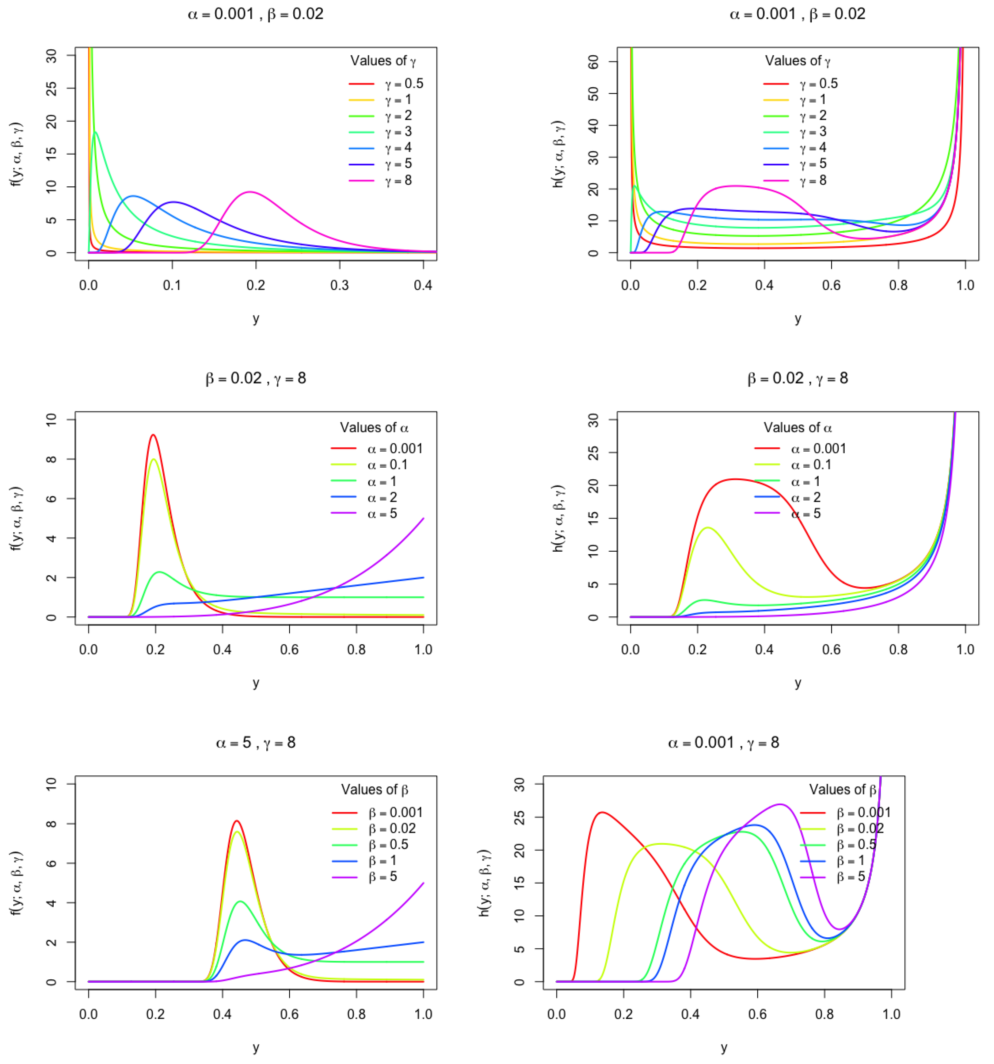
Figure 1 illustrates the behavior and shape of the PDF and HRF by assuming specific numerical values for the model parameters. The graphical representations highlight the flexibility and adaptability of the proposed model in capturing diverse data patterns. Based on the results presented in Figure 1, several key observations can be made:

• The proposed PDF exhibits a wide range of shapes, including decreasing, unimodal, and increasing forms. This versatility is particularly advantageous because it allows the model to accommodate various types of real-world data. For instance, the decreasing form may be suitable for modeling phenomena with high initial probabilities that taper off over time, while the unimodal shape can represent processes with a peak probability at a certain point. The increasing form, on the other hand, is useful for scenarios where the likelihood of an event grows over time. Such flexibility ensures that the model can be applied to different statistical and practical contexts.
• The corresponding HRF demonstrates even more diverse behaviors, including bathtub-shaped, increasing, increasing–decreasing–increasing, and upside-down bathtub followed by bathtub patterns. These variations are significant because they reflect different failure or risk trends commonly observed in reliability engineering, survival analysis, and other fields. For example, the bathtub-shaped HRF is characteristic of systems with high initial failure rates (early failures), a stable period (useful life), and an eventual increase due to wear-out (aging). Meanwhile, the increasing–decreasing–increasing pattern captures more complex scenarios where risk fluctuates non-monotonically. Such adaptability makes the model highly effective in fitting a broad spectrum of real-world data sets, enhancing its practical utility.

Overall, the proposed model’s ability to generate these varied PDF and HRF shapes underscores its robustness and wide applicability. By encompassing multiple forms, the model can more effectively represent empirical data, making it a valuable tool for statistical modeling and data analysis across various disciplines.

3. Mathematical Properties

This section delivers a rigorous and insightful exploration of pivotal theoretical advancements pertaining to the UMW distribution, elucidating its intrinsic structural and probabilistic characteristics through a meticulous analysis of quantiles, moments, the moment-generating function, skewness, and kurtosis, thereby enriching the foundational understanding of its behavior and broadening its theoretical applicability.

3.1. Quantiles

Given the CDF $F_Y(y;\alpha ,\beta ,\gamma )$ defined by Equation (3), the quantile function of the UMW distribution can be derived as $Q_Y\left(q\right)=F^{-1}\left(q\right),q\in (0, 1)$. Due to the analytical intractability of inverting the distribution function in closed form, the quantile values can be efficiently and accurately obtained numerically by solving the following non-linear equation.

$$\alpha log\left(y\right)-\beta {(-logy)}^{\gamma }-log\left(q\right)=0,$$

where $0<y<1$; $\alpha ,\beta \ge 0$ such that $\alpha +\beta >0$, $\gamma >0$, and $q\in (0, 1)$. This equation can be solved easily using the bisection method.

3.2. Moments

The $rth$ moment, around zero, for a random variable $Y\sim UMW$$(\alpha ,\beta ,\gamma )$ distribution is given by

$${\mu }_r^{\prime }=\sum _{k=0}^{\infty }{\displaystyle \frac{{(-1)}^k{\beta }^k}{k!{(r+\alpha )}^{\gamma k+1}}}\left\{\alpha \Gamma (\gamma k+1)+\beta \gamma {(r+\alpha )}^{1-\alpha }\Gamma (\gamma k+\gamma )\right\},$$

(7)

where $r=0,1,2\dots$, and $\Gamma (.)$ is the gamma function. Moreover, the moment-generating function can be reported as

$$M_Y\left(t\right)=\sum _{s=0}^{\infty }\sum _{k=0}^{\infty }{\displaystyle \frac{{(-1)}^k{t}^s{\beta }^k}{s!k!{(s+\alpha )}^{\gamma k+1}}}\left\{\alpha \Gamma (\gamma k+1)+\beta \gamma {(s+\alpha )}^{1-\alpha }\Gamma (\gamma k+\gamma )\right\}.$$

(8)

Using Equation (7), the mean, variance, skewness ($\mathcal{S}k\left(Y\right)$), and kurtosis ($\mathcal{K}u\left(Y\right)$) can be given by the respective equations listed below:

$${\mu }_1^{\prime }=\sum _{k=0}^{\infty }{\displaystyle \frac{{(-1)}^k{\beta }^k}{k!{(1+\alpha )}^{\gamma k+1}}}\left\{\alpha \Gamma (\gamma k+1)+\beta \gamma {(1+\alpha )}^{1-\alpha }\Gamma (\gamma k+\gamma )\right\},$$

(9)

$$V\left(Y\right)=\sum _{k=0}^{\infty }{\displaystyle \frac{{(-1)}^k{\beta }^k}{k!{(2+\alpha )}^{\gamma k+1}}}\left\{\alpha \Gamma (\gamma k+1)+\beta \gamma {(2+\alpha )}^{1-\alpha }\Gamma (\gamma k+\gamma )\right\}-{{\mu }_1^{\prime }}^2,$$

(10)

$$\mathcal{S}k\left(Y\right)={\displaystyle \frac{{\mu }_3^{\prime }-3{\mu }_1^{\prime }{\mu }_2^{\prime }+3{{\mu }_1^{\prime }}^3}{{\left(V\left(Y\right)\right)}^{3/2}}}$$

(11)

and

$$\mathcal{K}u\left(Y\right)={\displaystyle \frac{{\mu }_4^{\prime }-4{\mu }_1^{\prime }{\mu }_3^{\prime }+6{{\mu }_1^{\prime }}^2{\mu }_2^{\prime }-3{{\mu }_1^{\prime }}^4}{{\left(V\left(Y\right)\right)}^2}}.$$

(12)

Deriving closed-form solutions for many statistical measures, such as moments, skewness, and kurtosis, is often analytically intractable, particularly for complex or newly proposed probability distributions. When exact mathematical expressions are either too cumbersome or impossible to obtain, researchers frequently turn to numerical methods to explore the behavior of these quantities. Computational techniques provide a practical and efficient means to assess the convergence of associated series, validate theoretical results, and ensure the robustness of statistical models.

Given the challenges in obtaining explicit formulas, numerical approximation becomes indispensable. By evaluating key statistical measures across different parameter configurations, researchers can gain deeper insights into the distribution’s properties, including its central tendency, dispersion, asymmetry, and tail behavior. This approach not only supports theoretical derivations but also enhances the interpretability and applicability of the model in real-world scenarios.

Table 2. Descriptive statistics of the UMW distribution at $\beta =0.1$.

Measure	$\mathit{\gamma }\downarrow \mathit{\alpha }\to$	0.1	0.5	1.0	2.0	3.0	4.0	7.0
$E\left(Y\right)$	0.5	0.1638	0.3794	0.5301	0.6832	0.7608	0.8077	0.8789
	1.0	0.1667	0.3750	0.5238	0.6774	0.7561	0.8039	0.8765
	3.0	0.2358	0.3951	0.5254	0.6729	0.7522	0.8009	0.8752
	5.0	0.2875	0.4189	0.5344	0.6739	0.7519	0.8006	0.8750
	7.0	0.3151	0.4337	0.5411	0.6752	0.7521	0.8006	0.8750
$\mathrm{Var}\left(Y\right)$	0.5	0.0768	0.0993	0.0853	0.0548	0.0367	0.0260	0.0119
	1.0	0.0631	0.0901	0.0805	0.0533	0.0362	0.0258	0.0119
	3.0	0.0353	0.0679	0.0699	0.0515	0.0361	0.0261	0.0121
	5.0	0.0229	0.0549	0.0622	0.0497	0.0358	0.0261	0.0121
	7.0	0.0179	0.0484	0.0576	0.0483	0.0355	0.0261	0.0121
$\mathcal{S}k\left(Y\right)$	0.5	1.9573	2.2114	5.8814	24.2264	61.7552	124.4307	524.0429
	1.0	1.9502	2.4110	6.2151	24.8499	61.9803	124.0099	517.9699
	3.0	3.6186	4.1253	7.9216	25.6074	61.2560	120.8403	503.4262
	5.0	8.9522	6.5869	10.0574	27.1649	61.8812	120.4489	500.8145
	7.0	15.7047	8.6906	11.7764	28.5983	62.8389	120.8426	500.2055
$\mathcal{K}u\left(Y\right)$	0.5	4.8107	1.8879	1.7978	2.4819	3.1959	3.8027	5.0836
	1.0	4.7143	1.9469	1.8316	2.4720	3.1600	3.7509	5.0119
	3.0	5.6845	2.3038	1.8365	2.2967	2.9755	3.5916	4.9244
	5.0	8.3234	2.6291	1.7954	2.1157	2.8256	3.4991	4.9221
	7.0	10.8684	2.8576	1.7838	2.0002	2.7164	3.4271	4.9197

,

Table 3. Descriptive statistics of the UMW distribution at $\beta =1$.

Measure	$\mathit{\gamma }\downarrow \mathit{\alpha }\to$	0.1	0.5	1.0	2.0	3.0	4.0	7.0
$E\left(Y\right)$	0.5	0.5732	0.6546	0.7191	0.7933	0.8353	0.8627	0.9074
	1.0	0.5238	0.6000	0.6667	0.7500	0.8000	0.8333	0.8889
	3.0	0.4532	0.5292	0.6025	0.7022	0.7649	0.8072	0.8763
	5.0	0.4312	0.5103	0.5873	0.6928	0.7592	0.8037	0.8754
	7.0	0.4208	0.5020	0.5811	0.6894	0.7574	0.8026	0.8752
$\mathrm{Var}\left(Y\right)$	0.5	0.1295	0.0959	0.0695	0.0414	0.0275	0.0197	0.0093
	1.0	0.0805	0.0686	0.0556	0.0375	0.0267	0.0198	0.0099
	3.0	0.0244	0.0369	0.0413	0.0369	0.0292	0.0227	0.0115
	5.0	0.0149	0.0326	0.0406	0.0385	0.0309	0.0239	0.0119
	7.0	0.0119	0.0318	0.0411	0.0395	0.0317	0.0245	0.0120
$\mathcal{S}k\left(Y\right)$	0.5	3.7079	8.8129	19.4349	58.1719	126.4021	231.2504	836.4035
	1.0	6.2151	11.6898	22.0617	57.2337	116.5257	205.8796	714.1188
	3.0	25.2258	21.4384	26.1952	48.5647	88.9606	152.5219	542.5166
	5.0	45.7170	23.5623	25.1583	43.7877	80.0642	139.0163	515.6736
	7.0	59.2981	23.5497	24.0966	41.5320	76.5179	134.1807	508.5252
$\mathcal{K}u\left(Y\right)$	0.5	1.5853	2.0753	2.6709	3.6737	4.4395	5.0365	6.2121
	1.0	1.8316	2.0505	2.4000	3.0953	3.6964	4.2000	5.2841
	3.0	3.4451	2.5111	2.0272	2.1180	2.5955	3.1440	4.5663
	5.0	6.8218	3.1108	1.9922	1.8738	2.3729	2.9992	4.6226
	7.0	10.4935	3.4000	1.9690	1.7878	2.3159	2.9831	4.6866

and

Table 4. Descriptive statistics of the UMW distribution at $\beta =5$.

Measure	$\mathit{\gamma }\downarrow \mathit{\alpha }\to$	0.1	0.5	1.0	2.0	3.0	4.0	7.0
$E\left(Y\right)$	0.5	0.9352	0.9389	0.9428	0.9490	0.9537	0.9575	0.9654
	1.0	0.8361	0.8462	0.8571	0.8750	0.8889	0.9000	0.9231
	3.0	0.6139	0.6503	0.6888	0.7479	0.7907	0.8223	0.8803
	5.0	0.5344	0.5857	0.6386	0.7171	0.7712	0.8098	0.8764
	7.0	0.4961	0.5559	0.6168	0.7053	0.7646	0.8060	0.8756
$\mathrm{Var}\left(Y\right)$	0.5	0.0126	0.0108	0.0091	0.0068	0.0054	0.0044	0.0027
	1.0	0.0193	0.0174	0.0153	0.0122	0.0099	0.0082	0.0051
	3.0	0.0145	0.0189	0.0216	0.0218	0.0195	0.0167	0.0099
	5.0	0.0102	0.0203	0.0265	0.0281	0.0248	0.0206	0.0113
	7.0	0.0087	0.0222	0.0301	0.0318	0.0274	0.0223	0.0117
$\mathcal{S}k\left(Y\right)$	0.5	577.0437	735.1459	960.9091	1511.5906	2203.5079	3047.1535	6589.5472
	1.0	216.6983	263.6965	331.2708	498.6863	714.1188	983.5635	2175.9447
	3.0	133.6461	106.0717	103.3127	129.5327	180.9329	257.3317	683.0323
	5.0	149.8434	70.3439	60.9923	78.1086	117.3836	179.4241	557.9673
	7.0	152.7117	53.1348	45.5499	61.7377	98.1447	156.8770	528.2465
$\mathcal{K}u\left(Y\right)$	0.5	15.2734	15.2309	15.1549	14.9684	14.7714	14.5799	14.0764
	1.0	4.2456	4.4202	4.6222	4.9792	5.2841	5.5470	6.1542
	3.0	2.8909	2.6179	2.2552	2.1037	2.3108	2.6577	3.8681
	5.0	5.8425	3.4788	2.2556	1.8056	2.0606	2.5273	4.0928
	7.0	9.9957	3.8622	2.1983	1.7097	2.0397	2.5907	4.3129

provide comprehensive numerical evaluations of key statistical measures, including the mean ($E\left(Y\right)$), variance ($V\left(Y\right)$), $\mathcal{S}k\left(Y\right)$, and $\mathcal{K}u\left(Y\right)$ for the UMW distribution across varying values of the parameters, $\alpha ,$ $\beta$, and $\gamma$. The numerical results demonstrate that the UMW distribution exhibits remarkable shape flexibility, controlled by the parameters $\alpha$, $\beta$, and $\gamma$ as follows:

(i)

Increasing the $\alpha$ parameter consistently elevates the mean while reducing variance, accompanied by a pronounced increase in both skewness and kurtosis indicating a shift toward extreme right-skewed, leptokurtic distributions;

(ii)

An increase in the $\beta$ parameter produces a nuanced effect: it elevates the mean and skewness while paradoxically reducing both variance and kurtosis, highlighting a complex interplay between central tendency and tail behavior;

(iii)

The $\gamma$ parameter serves as a moderating factor: as $\gamma$ increases, both the mean and skewness systematically reduce across all configurations. Meanwhile, its effects on variance and kurtosis exhibit $\beta$-dependent behavior, sometimes counteracting and sometimes amplifying the influence of the remaining parameters.

This sophisticated interplay of parameters endows the UMW distribution with exceptional adaptability, making it particularly suitable for modeling diverse real-world phenomena that exhibit varying degrees of central tendency, dispersion, and tail heaviness. The observed patterns not only validate the distribution’s theoretical properties but also provide practical guidance for parameter selection in applied statistical modeling scenarios.

4. Parameter Estimation

Parameter estimation serves as a cornerstone of statistical inference, enabling researchers to deduce unknown model parameters from observed data. This process is fundamental to predictive modeling, hypothesis testing, and uncertainty quantification, with applications spanning scientific research, machine learning, and econometrics. Consider a simple random sample $Y_1,Y_2,\dots ,Y_n$ drawn from the UMW $\left(\theta \right)$ distribution with PDF given in Equation (4), where $\theta =(\alpha ,\beta ,\gamma )$ denotes the vector of unknown parameters. In this section, we derive estimates for $\theta$ using a maximum likelihood estimation (MLE) framework. Additionally, we derive asymptotic confidence intervals for these parameters, offering a robust measure of estimation uncertainty under large-sample conditions.

4.1. Maximum Likelihood Method

The maximum likelihood estimates (MLEs) of the parameters are obtained by maximizing the likelihood function. Let $y_1,y_2,\dots ,y_n$ denote the observed value of random sample of size n from the UMW distribution for the vector of parameters $\theta =(\alpha ,\beta ,\gamma )$. The likelihood function is given as

$$l\left(\theta \right)=\prod _{i=1}^{n}f(y_i;\theta ),$$

and the MLEs of the components of $\theta$ are the values of $\theta$, say $\widehat{\theta }$, which maximize the likelihood function. That is, $\widehat{\theta }$ satisfies

$${\widehat{\theta }}_{\mathrm{MLE}}=arg\underset{\theta }{max}l\left(\theta \right).$$

Equivalently, the MLEs of the parameters are obtained by maximizing the log-likelihood function, which can be written as

$$L\left(\theta \right)=(\gamma -1)\sum _{i=1}^{n}log{y}_i-\beta \sum _{i=1}^n{(-log{y}_i)}^{\gamma }+\sum _{i=1}^{n}log(\alpha +\beta \gamma {(-log{y}_i)}^{\gamma -1}).$$

(13)

To maximize the log-likelihood function, we solve the system of non-linear likelihood equations obtained by differentiating Equation (13). The required score vector components for these equations are given below:

$$S_1(\alpha ,\beta ,\gamma )={\displaystyle \frac{\partial L}{\partial \alpha }}=\sum _{i=1}^n{\displaystyle \frac{1}{\alpha +\beta \gamma K(y_i;\gamma )}};$$

(14)

$$S_2(\alpha ,\beta ,\gamma )={\displaystyle \frac{\partial L}{\partial \beta }}=\sum _{i=1}^n{\displaystyle \frac{\gamma K(y_i;\gamma )}{\alpha +\beta \gamma K(y_i;\gamma )}}-\sum _{i=1}^n{(-log{y}_i)}^{\gamma };$$

(15)

$$S_3(\alpha ,\beta ,\gamma )={\displaystyle \frac{\partial L}{\partial \gamma }}=\beta \sum _{i=1}^n{\displaystyle \frac{K(y_i;\gamma )+\gamma K(y_i;\gamma )M\left(y_i\right)}{\alpha +\beta \gamma K(y_i;\gamma )}}+\sum _{i=1}^{n}log{y}_i-\beta \sum _{i=1}^n{(-log{y}_i)}^{\gamma }M\left(y_i\right).$$

(16)

where $K(y_i;\gamma )={(-log{y}_i)}^{\gamma -1}$ and $M\left(y_i\right)=log(-log{y}_i)$. The information matrix is a three-by-three symmetric matrix given by

$$I(\alpha ,\beta ,\gamma )=\left[\begin{array}{ccc}{I}_{11}(\alpha ,\beta ,\gamma )& I_{12}(\alpha ,\beta ,\gamma )& I_{13}(\alpha ,\beta ,\gamma )\\ I_{12}(\alpha ,\beta ,\gamma )& I_{22}(\alpha ,\beta ,\gamma )& I_{23}(\alpha ,\beta ,\gamma )\\ I_{13}(\alpha ,\beta ,\gamma )& I_{23}(\alpha ,\beta ,\gamma )& I_{33}(\alpha ,\beta ,\gamma )\end{array}\right]$$

where

$$\begin{array}{ccc}\hfill I_{11}& =& -{\displaystyle \frac{\partial S_1}{\partial \alpha }}=\sum _{i=1}^n{\displaystyle \frac{1}{{\left(\alpha +\beta \gamma K(y_i;\gamma )\right)}^2}};\hfill \\ \hfill I_{12}& =& -{\displaystyle \frac{\partial S_1}{\partial \beta }}=\sum _{i=1}^n{\displaystyle \frac{\gamma K(y_i;\gamma )}{{\left(\alpha +\beta \gamma K(y_i;\gamma )\right)}^2}};\hfill \\ \hfill I_{13}& =& -{\displaystyle \frac{\partial S_1}{\partial \gamma }}=\sum _{i=1}^n{\displaystyle \frac{\beta K(y_i;\gamma )+\beta \gamma K(y_i;\gamma )M\left(y_i\right)}{{\left(\alpha +\beta \gamma K(y_i;\gamma )\right)}^2}};\hfill \\ \hfill I_{22}& =& -{\displaystyle \frac{\partial S_2}{\partial \beta }}=\sum _{i=1}^n{\displaystyle \frac{{\gamma }^2{K}^2(y_i;\gamma )}{{\left(\alpha +\beta \gamma K(y_i;\gamma )\right)}^2}};\hfill \end{array}$$

$$\begin{array}{c}{I}_{23}=-{\displaystyle \frac{\partial S_2}{\partial \gamma }}=\sum _{i=1}^n\{-{\displaystyle \frac{\left(K(y_i;\gamma )+\gamma K(y_i;\gamma )M\left(y_i\right)\right)}{\alpha +\beta \gamma K(y_i;\gamma )}}\hfill \\ \hspace{1em}\hspace{1em}\hspace{1em}\hspace{1em}\hspace{1em}\hspace{1em}\hspace{1em}-{\displaystyle \frac{\beta \gamma \left(K(y_i;\gamma )+\gamma K(y_i;\gamma )M\left(y_i\right)\right)K(y_i;\gamma )}{{\left(\alpha +\beta \gamma K(y_i;\gamma )\right)}^2}}\}+\sum _{i=1}^n{(-log{y}_i)}^{\gamma }M\left(y_i\right);\hfill \end{array}$$

$$\begin{array}{c}\hfill I_{33}=-{\displaystyle \frac{\partial S_3}{\partial \gamma }}=\sum _{i=1}^n\left\{-{\displaystyle \frac{\beta \gamma M^2\left(y_i\right)K(y_i;\gamma )+2\beta M\left(y_i\right)}{\alpha +\beta \gamma K(y_i;\gamma )}}\right.+\left(\beta K(y_i;\gamma )+\beta \gamma M\left(y_i\right)K(y_i;\gamma )\right)\hfill \\ \hfill \left.\times \left({\displaystyle \frac{\beta K(y_i;\gamma )}{{\left(\alpha +\beta \gamma K(y_i;\gamma )\right)}^2}}+{\displaystyle \frac{\beta \gamma M\left(y_i\right)K(y_i;\gamma )}{{\left(\alpha +\beta \gamma K(y_i;\gamma )\right)}^2}}\right)\right\}+\beta \sum _{i=1}^n{M}^2\left(y_i\right){(-log\left(y\left(i\right)\right))}^{\gamma }.\end{array}$$

To derive the MLEs of the model parameters $\alpha$, $\beta$, and $\gamma$, we solve the following system of equations:

$$S_1(\alpha ,\beta ,\gamma )=0,S_2(\alpha ,\beta ,\gamma )=0\mathrm{and}{S}_3(\alpha ,\beta ,\gamma )=0.$$

The MLEs of the model parameters are the solution of the likelihood equations such that the information matrix is positive definite. Using advanced numerical methods in R, we can efficiently solve these equations to high precision, uncovering their roots with computational rigor.

4.2. Asymptotic Confidence Intervals

When MLEs of model parameters lack closed-form solutions, their exact sampling distributions become analytically intractable, making precise confidence intervals unavailable. In such cases, we must resort to the asymptotic properties of MLEs to construct approximate confidence intervals.

The MLE $\widehat{\mathit{\theta }}=(\widehat{\alpha },\widehat{\beta },\widehat{\gamma })$ of the parameter vector $\mathit{\theta }=(\alpha ,\beta ,\gamma )$ follows an asymptotic normal distribution:

$$\widehat{\mathit{\theta }}\stackrel{\mathrm{approx}}{\sim }\mathcal{N}\left(\mathit{\theta },I^{-1}\left(\mathit{\theta }\right)\right),$$

where $I\left(\mathit{\theta }\right)$ is the Fisher information matrix. The $(1-\vartheta )100\%$ confidence interval for each parameter ${\theta }_j$ is given by

$${\widehat{\theta }}_j\pm z_{\vartheta /2}·\mathrm{SE}\left({\widehat{\theta }}_j\right),j=1,2,3,$$

where

• $\mathrm{SE}\left({\widehat{\theta }}_j\right)=\sqrt{\mathrm{Var}\left({\widehat{\theta }}_j\right)}$ is the standard error of ${\widehat{\theta }}_j$, ;
• $\mathrm{Var}\left({\widehat{\theta }}_j\right)$ is the j-th diagonal element of the inverse Fisher information matrix $I^{-1}\left(\widehat{\mathit{\theta }}\right)$;
• $z_{\vartheta /2}$ is the critical value from the standard normal distribution such that $P(Z>z_{\vartheta /2})=\vartheta /2$.

5. Simulation Studies

A comprehensive simulation study is conducted using R statistical software to evaluate the performance of the MLEs for the parameters of the UMW distribution. The study is designed to assess the consistency, efficiency, and asymptotic properties of the estimators under varying sample sizes and parameter configurations. The simulation framework employed a systematic approach to ensure robustness, incorporating 10,000 iterations per sample size to mitigate stochastic variability and provide reliable estimates of the statistical properties of the estimators.

The investigation spanned nine sample sizes (ranging from small to large), namely $n=20,50,80,100,150,200,300,400,500$, enabling a thorough examination of the estimators’ behavior across different data availability scenarios. Four distinct parameter configurations are selected to test the estimators under diverse distributional shapes and scales:

• $\alpha =0.5,\beta =0.5,\gamma =0.8$
• $\alpha =0.8,\beta =1,\gamma =1.5$
• $\alpha =1.2,\beta =1.5,\gamma =3$
• $\alpha =1.2,\beta =0.5,\gamma =0.2$

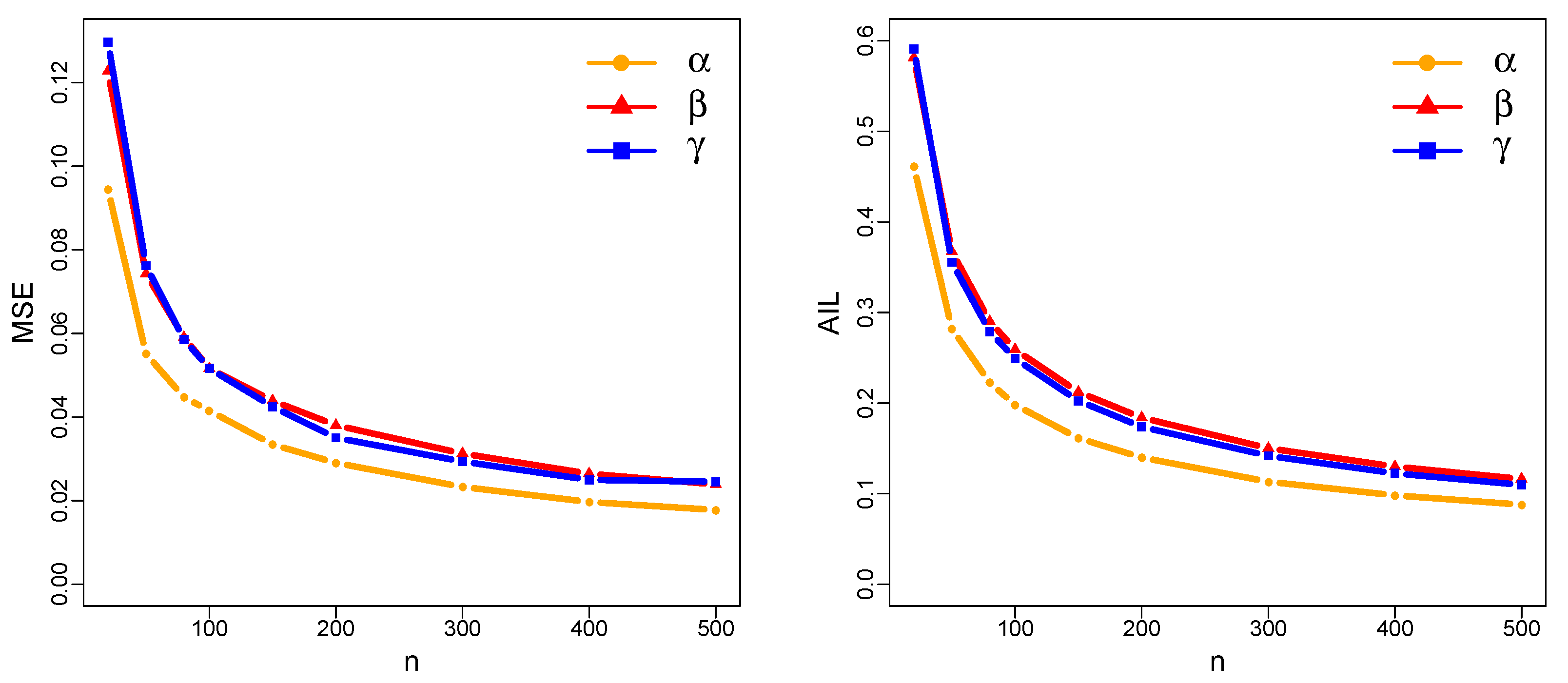
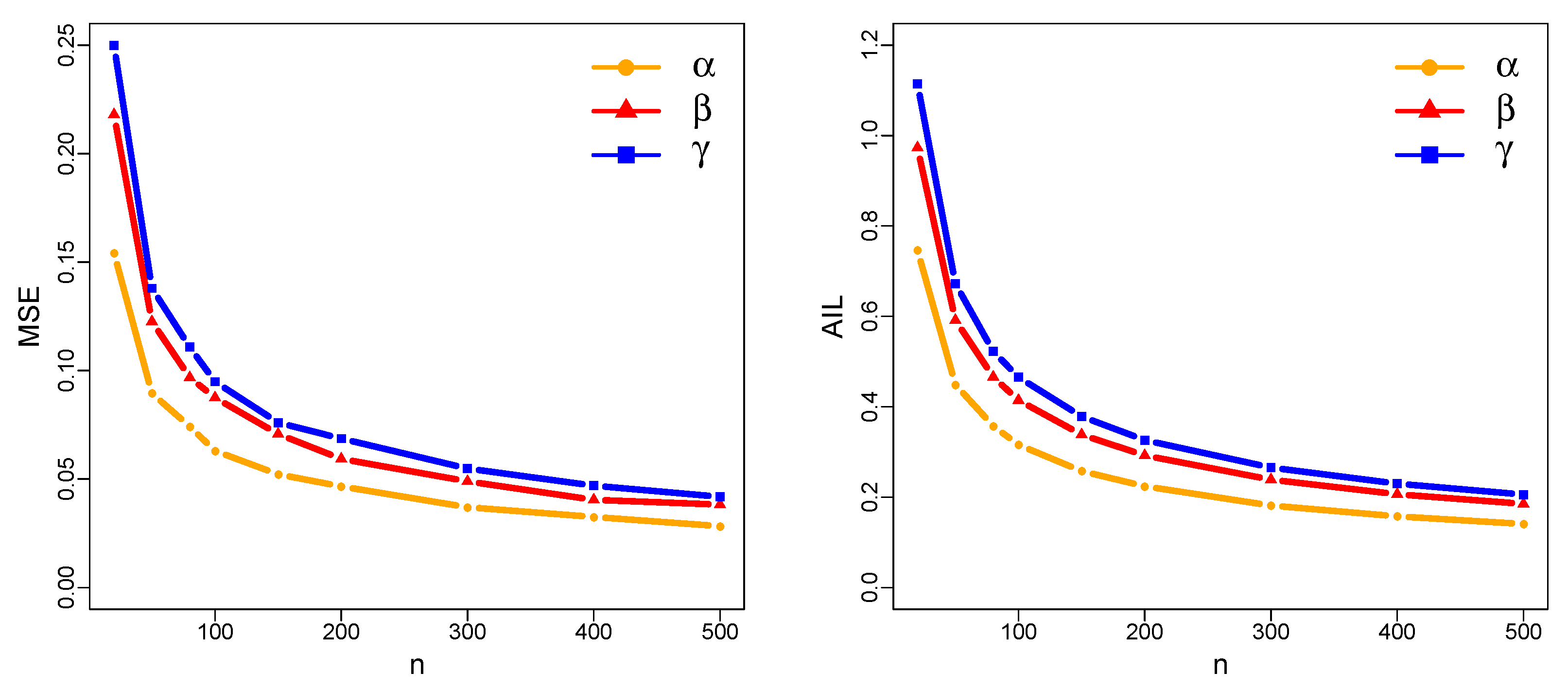
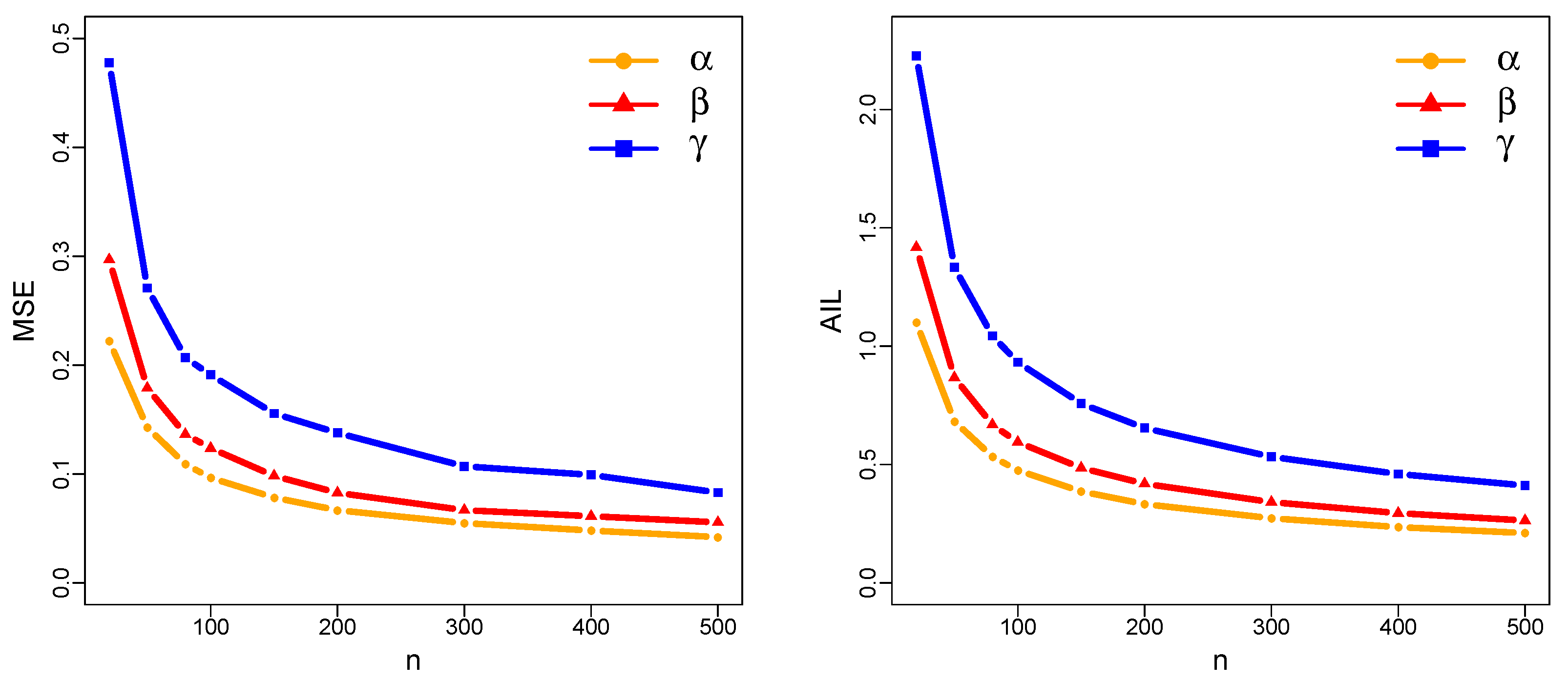
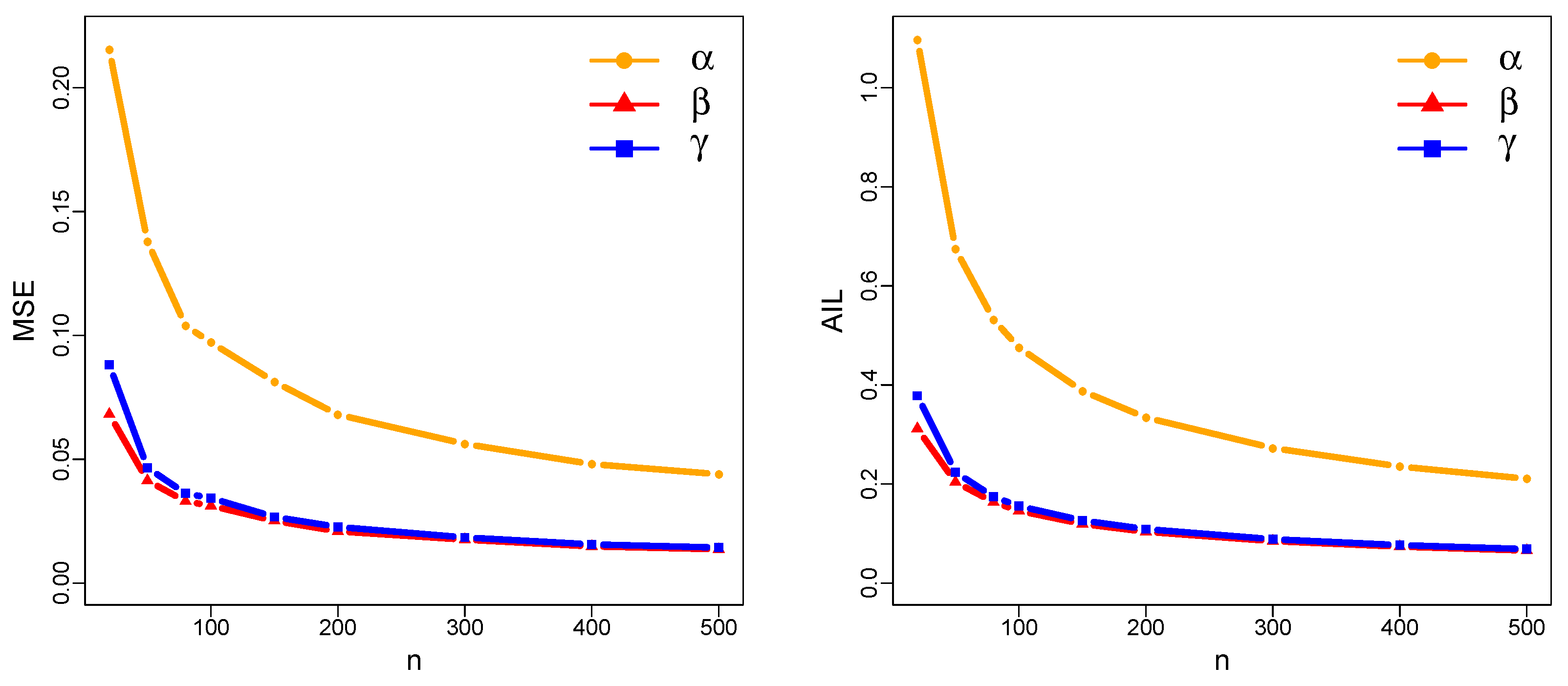
These configurations are chosen to represent a spectrum of plausible real-world scenarios, ensuring that the evaluation is not limited to a single parametric regime. To ensure the robustness and reliability of the numerical optimization, a sensitivity analysis was performed. For each configuration and sample size, the estimation algorithm was initiated from multiple starting points within a reasonable neighborhood of the true parameters. The results demonstrated a high degree of convergence to the same solution, indicating that the MLE for the UMW distribution is robust to the choice of initial values across the tested scenarios. The iterative algorithms consistently converged without computational issues, confirming the numerical stability of the estimation procedure. This robustness provides confidence in the reliability of the presented average of MLE (AMLE), mean square error (MSE), average interval length (AIL), and coverage probability (CP) results. The simulation’s performance is rigorously scrutinized through a selection of pivotal metrics, AMLE, MSE, AIL, and CP, each illuminating a distinct facet of estimator quality. The MSE stands as the bedrock of predictive accuracy, quantifying average squared deviation between the estimated and true parameter values, serving as a composite indicator of bias and variance. A declining MSE with increasing sample size signals consistency and efficiency of the MLE. Complementing this, the AIL reflects the precision of the confidence intervals for the model parameters. Narrower intervals indicate higher precision while maintaining valid coverage. Yet, precision alone is insufficient without validity; this is where CP ascends as the definitive arbiter of interval trustworthiness. By assessing the empirical frequency with which these intervals encompass the true parameter, a CP aligning with the nominal level underscores the methodological rigor and reliability of the inferential framework. Together, these metrics forge a comprehensive evaluation paradigm, balancing accuracy, precision, and statistical fidelity. The simulation outcomes are meticulously documented in

Table 5. Simulation results for the UMW parameters.

n	Parameter	$\mathit{\alpha }=0.5,\mathit{\beta }=0.5,\mathit{\gamma }=0.8$				$\mathit{\alpha }=0.8,\mathit{\beta }=1,\mathit{\gamma }=1.5$
		AMLE	MSE	AIL	CP	AMLE	MSE	AIL	CP
	$\alpha$	0.5265	0.0945	0.4615	95.1%	0.8515	0.1542	0.7464	95.4%
20	$\beta$	0.5053	0.1227	0.5812	92.5%	1.0555	0.2180	0.9732	93.9%
	$\gamma$	0.8573	0.1297	0.5911	94.8%	1.6116	0.2499	1.1144	94.2%
	$\alpha$	0.5093	0.0551	0.2823	95.7%	0.8098	0.0895	0.4489	95.5%
50	$\beta$	0.5016	0.0743	0.3674	94.2 %	1.0128	0.1226	0.5914	94.4%
	$\gamma$	0.8182	0.0762	0.3555	94.3%	1.5464	0.1379	0.6723	95.8%
	$\alpha$	0.5079	0.0446	0.2226	96.4%	1.5464	0.1379	0.6723	95.8%
80	$\beta$	0.4999	0.0591	0.2900	94.7%	1.0098	0.0968	0.4659	94.4%
	$\gamma$	0.8135	0.0585	0.2789	95.1%	1.5239	0.1108	0.5224	94.1%
	$\alpha$	0.5053	0.0415	0.1981	94.8%	0.8056	0.0629	0.3158	95.7%
100	$\beta$	0.4986	0.0516	0.2591	95.2%	1.0029	0.0875	0.4144	93.9%
	$\gamma$	0.8135	0.0516	0.2492	95.7%	1.5195	0.0949	0.4654	96.4%
	$\alpha$	0.5039	0.0334	0.1613	94.9%	0.8045	0.0522	0.2575	94.7%
150	$\beta$	0.5008	0.0439	0.2122	95.5%	1.0034	0.0708	0.3382	95.1%
	$\gamma$	0.8104	0.0425	0.2025	95.1%	1.5131	0.0760	0.3784	95.4 %
	$\alpha$	0.5048	0.0290	0.1399	95.2%	0.8082	0.0466	0.2240	94.3%
200	$\beta$	0.5014	0.0380	0.1839	94.3%	1.0005	0.0593	0.2922	94.9%
	$\gamma$	0.8036	0.0351	0.1738	95.4%	1.5069	0.0686	0.3261	95.0%
	$\alpha$	0.5004	0.0233	0.1132	94.5%	0.8016	0.0370	0.1814	95.1%
300	$\beta$	0.5014	0.0313	0.1502	95.1%	1.0012	0.0489	0.2386	94.9%
	$\gamma$	0.8034	0.0294	0.1418	96.1%	1.5024	0.0548	0.2654	94.3%
	$\alpha$	0.5010	0.0197	0.0982	94.4%	0.8034	0.0325	0.1575	95.1%
400	$\beta$	0.5008	0.0265	0.1299	94.2%	0.9996	0.0404	0.2064	95.2%
	$\gamma$	0.8014	0.0249	0.1225	95.6%	1.5031	0.0469	0.2298	93.8%
	$\alpha$	0.5014	0.0178	0.0879	94.6%	0.8019	0.0283	0.1406	95.2%
500	$\beta$	0.5002	0.0239	0.1162	94.7%	1.0030	0.0382	0.1851	94.9%
	$\gamma$	0.8026	0.0245	0.1098	94.4%	1.5042	0.0418	0.2057	94.8%

and

Table 6. Simulation results for the UMW parameters.

n	Parameter	$\mathit{\alpha }=1.2,\mathit{\beta }=1.5,\mathit{\gamma }=3$				$\mathit{\alpha }=1.2,\mathit{\beta }=0.5,\mathit{\gamma }=0.2$
		AMLE	MSE	AIL	CP	AMLE	MSE	AIL	CP
	$\alpha$	1.2554	0.2222	1.1004	95.2%	1.2515	0.2154	1.0969	95.8%
20	$\beta$	1.5841	0.2969	1.4175	94.7%	0.1915	0.06817	0.3119	88.2%
	$\gamma$	3.2173	0.4777	2.2265	94.6%	0.5468	0.0882	0.3783	94.7%
	$\alpha$	1.2314	0.1428	0.6826	94.3%	1.2166	0.1379	0.6744	94.7%
50	$\beta$	1.5538	0.1789	0.8672	95.8%	0.1969	0.0414	0.2039	92.9%
	$\gamma$	3.0721	0.2708	1.3327	94.4%	0.5156	0.0466	0.2238	95.0%
	$\alpha$	1.2174	0.1091	0.5335	95.8%	1.2140	0.1039	0.5321	95.7%
80	$\beta$	1.5188	0.1365	0.6683	95.2%	0.1997	0.0330	0.1633	94.2%
	$\gamma$	3.0466	0.2069	1.0438	95.3%	0.5083	0.0362	0.1743	94.5%
	$\alpha$	1.2127	0.0965	0.4754	96.3%	1.2129	0.0972	0.4754	95.3%
100	$\beta$	1.5122	0.1237	0.5947	94.4%	0.1991	0.0312	0.1458	93.5%
	$\gamma$	3.0425	0.1911	0.9322	95.4%	0.5074	0.0343	0.1554	94.0%
	$\alpha$	1.2076	0.0784	0.3865	94.7%	1.2117	0.0813	0.3878	94.8%
150	$\beta$	1.5144	0.0983	0.4857	96.3%	0.1994	0.0251	0.1194	93.2%
	$\gamma$	3.0277	0.1556	0.7575	96.2%	0.5054	0.0267	0.1264	94.5%
	$\alpha$	1.2009	0.0668	0.3329	95.0%	1.2055	0.0680	0.3341	95.6%
200	$\beta$	1.5093	0.0828	0.4189	95.8%	0.1998	0.0209	0.1036	93.9%
	$\gamma$	3.0239	0.1378	0.6541	95.4%	0.5038	0.0227	0.1089	93.9%
	$\alpha$	1.2069	0.0549	0.2731	94.8%	1.2045	0.0562	0.2726	95.3%
300	$\beta$	1.5067	0.0668	0.3414	96.4%	0.2000	0.0175	0.0847	94.3%
	$\gamma$	3.0159	0.1071	0.5327	94.7 %	0.5011	0.0184	0.0885	94.3%
	$\alpha$	1.2028	0.0481	0.2357	95.4%	1.2008	0.0481	0.2353	94.7%
400	$\beta$	1.5026	0.0613	0.2948	93.4 %	0.2008	0.0148	0.0736	94.2%
	$\gamma$	3.0099	0.0992	0.4601	95.0 %	0.5009	0.0156	0.0766	94.1%
	$\alpha$	1.2018	0.0421	0.2107	95.2%	1.2013	0.0439	0.2106	94.3%
500	$\beta$	1.5026	0.0556	0.2636	95.4%	0.2002	0.0137	0.0657	94.7%
	$\gamma$	3.0095	0.0829	0.4115	95.2%	0.5011	0.0143	0.0685	94.9%

, with the corresponding MSE and AIL trends visually synthesized in Figure 2, Figure 3, Figure 4 and Figure 5. A rigorous analysis of these tabulated results and graphical representations yields the following key insights:

• The MSE exhibited a monotonic decrease as the sample size increased across all parameter configurations. This trend robustly supports the asymptotic unbiasedness and consistency of the MLE method, as estimators converge toward their true values with larger data sets.
• The AIL contracted systematically with larger sample sizes, indicating sharper and more informative confidence intervals.
• The CP consistently approached the nominal $95\%$ level across all sample sizes, particularly for $n>100$. This alignment confirms that the MLE-based confidence intervals are statistically valid, even for smaller samples in most cases. The coverage probability for the parameter $\beta$ is notably low (88.2%) when $n=20$ in the fourth configuration ($\alpha =1.2,\beta =0.5,\gamma =0.2$). This occurs because a small shape parameter ($\gamma =0.2$) causes more extreme distributional behavior, making estimation difficult with very limited data. The standard normal approximation used for confidence intervals becomes less reliable here, leading to under-coverage. Fortunately, this is only a small-sample issue, the coverage quickly improves to 92.9% at $n=50$ and reaches acceptable levels (≥93.2%) for $n\ge 150$. This suggests that although MLE is generally reliable, users should be cautious when interpreting results from very small samples, especially in skewed models. Future studies might improve small-sample inference using bias-corrected or profile likelihood methods.

The simulation outcomes underscore the theoretical robustness of MLE for the UMW distribution, with empirical results aligning closely with asymptotic expectations. The observed MSE decay and AIL reduction validate the efficiency of the estimators, while the CP adherence reinforces their reliability for practical inference.

6. Real Data Analysis

This section evaluates the flexibility and performance of the UMW model using three real-world data sets, comparing it against seven established models: UW, ULFR, UR, UE, Beta, Kumaraswamy (Kum), and Topp–Leone (TL).

The assessment employs multiple goodness-of-fit criteria: the negative log-likelihood (-L), Akaike information criterion (AIC), consistent AIC (CAIC), Hannan–Quinn information criterion (HQIC), Anderson–Darling ($A^{*}$), and Cramér–von Mises ($W^{*}$). The Kolmogorov–Smirnov (K–S) test and its p-value further evaluate the fit between empirical and theoretical distributions. The results confirm the UMW model’s strong performance, supporting its suitability for modeling unit interval data.

The first data set, from [16], records kidney dialysis patients’ infection times (in months). The second, from [17], captures the failure times of an airplane’s air conditioning system (in hours). The third, from [18], comprises 22 observations of P3 algorithm computing times.

Table 7. Descriptive statistics of the three real data sets.

Data	Min.	Mean	Q1	Median	Q3	Var	Skewness	Kurtosis	Max.
Kidney dialysis data	0.0833	0.3774	0.2083	0.3000	0.4833	0.0611	0.7651	2.4219	0.9167
Air conditioning data	0.0038	0.2249	0.0472	0.0830	0.3132	0.0736	1.6936	4.9667	0.9849
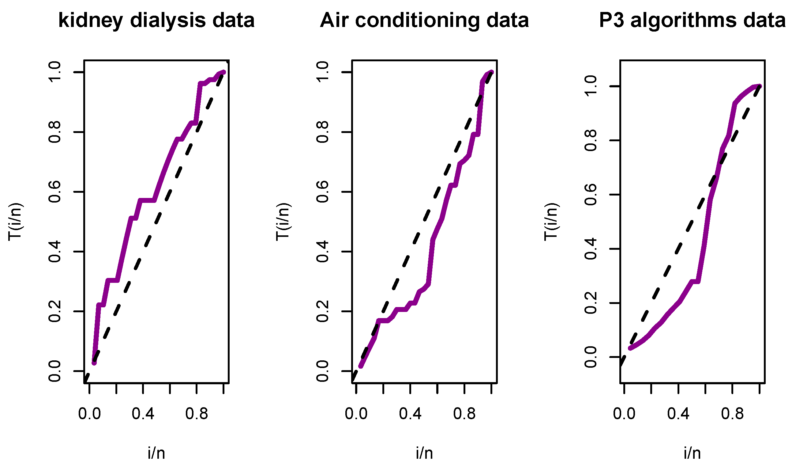
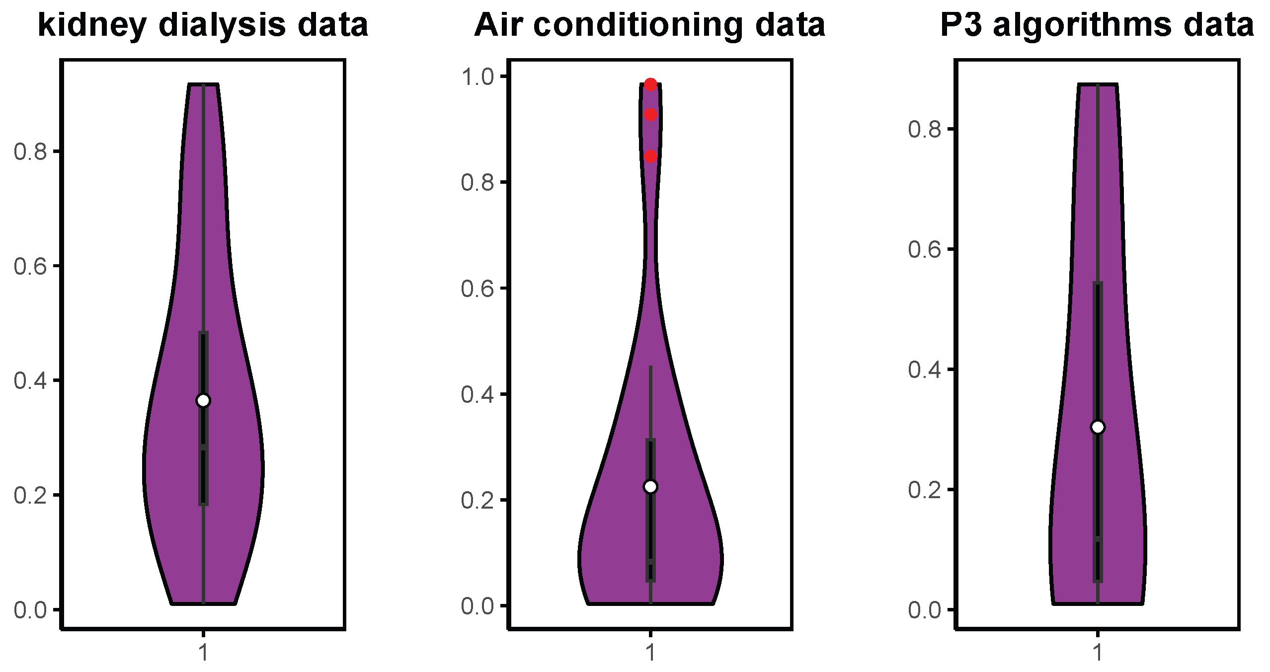
P3 algorithm data	0.0100	0.3039	0.0470	0.1180	0.5435	0.1010	0.7114	1.8838	0.8740

summarizes the data sets’ descriptive statistics. Kidney dialysis times show the lowest skewness and variability, while air conditioning data exhibits extreme right-skewness and outliers. The P3 algorithm times display high variance but moderate skewness, reflecting distinct analytical requirements. Nonparametric visualizations including total time on test (TTT) plot and violin plot are presented in Figure 6 and Figure 7 to illustrate the data distributions.

The TTT plots in Figure 6 provide insights into the hazard rate behavior of the three data sets:

• Kidney Dialysis Data: The TTT plot initially displays a concave shape, gradually transitioning to a linear trend. This suggests a decreasing hazard rate in the early phase, followed by a roughly constant hazard rate.
• Air Conditioning Data: The plot is approximately linear throughout, indicating a constant hazard rate, which is typical of an exponential distribution.
• P3 Algorithm Data: This plot shows a convex shape initially, followed by a concave trend. Such a pattern is characteristic of a bathtub-shaped hazard rate, implying an increasing failure rate at the beginning and a decreasing rate thereafter. This indicates that the UMW with $\gamma >1$ may be appropriate.

The violin plots in Figure 7 provide insight into the distributional characteristics of three real-world data sets:

• Kidney Dialysis Data: The distribution is approximately symmetric with a moderate spread, centered around the median. The density appears fairly uniform, indicating that the data is evenly distributed without notable skewness or extreme outliers.
• Air Conditioning Data: This data set exhibits strong right-skewness. The density is concentrated near lower values, with a long tail stretching toward higher values. A few visible outliers highlight the presence of extreme observations.
• P3 Algorithm Data: The data is also right-skewed, with most values clustered at the lower end. Unlike the air conditioning data, it lacks prominent outliers and displays a smoother decline in density toward the upper range.

Table 8. The MLE estimates and corresponding SE for the kidney dialysis data.

Model	$\widehat{\mathit{\alpha }}$	$\widehat{\mathit{\beta }}$	$\widehat{\mathit{\gamma }}$	$\mathit{SE}\left(\widehat{\mathit{\alpha }}\right)$	$\mathit{SE}\left(\widehat{\mathit{\beta }}\right)$	$\mathit{SE}\left(\widehat{\mathit{\gamma }}\right)$
UMW	0.4371	0.0897	3.6139	0.1960	0.1243	1.4790
UW	0.6125	1.6991	-	0.1424	0.2669	-
ULFR	0.2064	0.3931	-	0.1815	0.1334	-
UR	0.5222	-	-	0.0987	-	-
UE	0.7623	-	-	0.1441	-	-
Beta	1.3568	2.1058	-	0.3332	0.5497	-
kum	1.2651	2.0797	-	0.2544	0.5714	-
TL	1.3779	-	-	0.2604	-	-

,

Table 9. The MLE estimates and corresponding SE for the air conditioning data.

Model	$\widehat{\mathit{\alpha }}$	$\widehat{\mathit{\beta }}$	$\widehat{\mathit{\gamma }}$	$\mathit{SE}\left(\widehat{\mathit{\alpha }}\right)$	$\mathit{SE}\left(\widehat{\mathit{\beta }}\right)$	$\mathit{SE}\left(\widehat{\mathit{\gamma }}\right)$
UMW	0.2071	0.0250	2.9426	0.0999	0.0348	0.8629
UW	0.2787	1.4561	-	0.0858	0.2262	-
ULFR	0.1485	0.1004	-	0.0886	0.0335	-
UR	0.1498	-	-	0.0274	-	-
UE	0.3351	-	-	0.0612	-	-
Beta	0.5142	1.3430	-	0.1118	0.3643	-
kum	0.5451	1.3837	-	0.1148	0.3362	-
TL	0.6017	-	-	0.1099	-	-

,

Table 10. The MLE estimates and corresponding SE for the P3 algorithm data.

Model	$\widehat{\mathit{\alpha }}$	$\widehat{\mathit{\beta }}$	$\widehat{\mathit{\gamma }}$	$\mathit{SE}\left(\widehat{\mathit{\alpha }}\right)$	$\mathit{SE}\left(\widehat{\mathit{\beta }}\right)$	$\mathit{SE}\left(\widehat{\mathit{\gamma }}\right)$
UMW	0.3571	0.0054	3.8185	0.1134	0.0089	1.1726
UW	0.4003	1.2259	-	0.1263	0.2213	-
ULFR	0.3042	0.0662	-	0.1390	0.0432	-
UR	0.1672	-	-	0.0356	-	-
UE	0.8194	-	-	0.1747	-	-
Beta	0.5539	1.2198	-	0.1423	0.3758	-
kum	0.5718	1.2306	-	0.1478	0.3483	-
TL	0.6778	-	-	0.1445	-	-

,

Table 11. The $-L$, AIC, BIC, CAIC, HQIC, $W^{*}$, $A^{*}$, $K-S$, and corresponding p-values derived from using eight competitive models for the kidney dialysis data.

Model	$-\mathit{L}$	AIC	BIC	CAIC	HQIC	${\mathit{W}}^{*}$	${\mathit{A}}^{*}$	$\mathit{K}-\mathit{S}$	p-Value
UMW	−6.3169	−6.6339	−2.6373	−5.6339	−5.4121	0.0381	0.2819	0.0879	0.9820
UW	−5.0611	−6.1223	−3.4579	−5.6423	−5.3077	0.0659	0.4415	0.1240	0.7824
ULFR	−5.4608	−6.9215	−4.2571	−6.4415	−6.1069	0.0483	0.3489	0.1114	0.8779
UR	−4.4825	−6.9650	−5.6328	−6.8112	−6.5577	0.0557	0.3833	0.1579	0.4869
UE	1.8933	5.7866	7.1188	5.9404	6.1938	0.2606	1.4695	0.2758	0.0283
Beta	−3.7776	−3.5552	−0.8908	−3.0752	−2.7407	0.1101	0.6859	0.1412	0.6321
kum	−3.6625	−3.3249	−0.6606	−2.8449	−2.5104	0.1136	0.7049	0.1377	0.6629
TL	−3.8524	−5.7049	−4.3727	−5.5510	−5.2976	0.1067	0.6679	0.1442	0.6056

,

Table 12. The $-L$, AIC, BIC, CAIC, HQIC, $W^{*}$, $A^{*}$, $K-S$, and corresponding p-values derived from using eight competitive models for the air conditioning system data.

Model	$-\mathit{L}$	AIC	BIC	CAIC	HQIC	${\mathit{W}}^{*}$	${\mathit{A}}^{*}$	$\mathit{K}-\mathit{S}$	p-Value
UMW	−18.3687	−30.7375	−26.5339	−29.8144	−29.3927	0.0754	0.4625	0.1102	0.8596
UW	−15.1924	−26.3847	−23.5823	−25.9403	−25.4882	0.1593	1.0192	0.1741	0.3228
ULFR	−17.4207	−30.8414	−28.0390	−30.3969	−29.9448	0.1055	0.6546	0.1515	0.4969
UR	−12.7731	−23.5462	−22.1449	−23.4033	−23.0979	0.1254	0.7933	0.1262	0.7260
UE	35.9335	73.8671	75.2683	74.0099	74.3153	0.6164	3.4108	0.6626	<0.0001
Beta	−13.2463	−22.4926	−19.6902	−22.0482	−21.5961	0.2173	1.3859	0.1958	0.2003
kum	−13.5389	−23.0778	−20.2754	−22.6334	−22.1813	0.2109	1.3470	0.1879	0.2403
TL	−11.9802	−21.9604	−20.5592	−21.8175	−21.5121	0.2379	1.5103	0.1939	0.2095

and

Table 13. The $-L$, AIC, BIC, CAIC, HQIC, $W^{*}$, $A^{*}$, $K-S$, and corresponding p-values derived from using eight competitive models for the computing time of P3 algorithm data.

Model	$-\mathit{L}$	AIC	BIC	CAIC	HQIC	${\mathit{W}}^{*}$	${\mathit{A}}^{*}$	$\mathit{K}-\mathit{S}$	p-Value
UMW	−9.5357	−13.0714	−9.7982	−11.7380	−11.7380	0.0425	0.2879	0.1228	0.8944
UW	−7.1755	−10.3509	−8.1689	−9.7194	−9.8369	0.1048	0.6406	0.1833	0.4508
ULFR	−7.9048	−11.8096	−9.6275	−11.1779	−11.2955	0.0827	0.5146	0.1597	0.6286
UR	−2.7357	−3.4713	−2.3803	−3.2713	−3.2143	0.0795	0.4966	0.2423	0.1511
UE	3.0758	8.1516	9.2427	8.3516	8.4086	0.1621	0.9582	0.4416	0.0004
Beta	−6.7819	−9.5639	−7.3818	−8.9323	−9.0498	0.1173	0.7123	0.2002	0.3413
kum	−6.8436	−9.6872	−7.5052	−9.0557	−9.1732	0.1158	0.7037	0.1963	0.3650
TL	−5.4982	−8.9965	−7.9055	−8.7965	−8.7395	0.1249	0.7557	0.1848	0.4401

present the MLEs with their corresponding standard errors (SEs) along with the goodness-of-fit criteria for the competing models applied to the three data sets. The results demonstrate that the UMW distribution consistently outperforms its counterparts across key statistical measures, including the log-likelihood, AIC, BIC, CAIC, HQIC, and other nonparametric criteria. These comparative assessments highlight the UMW distribution’s superior flexibility and accuracy in modeling all three real data sets. Notably, its ability to provide a tighter fit compared to other distributions suggests that it is a more suitable choice for capturing the underlying patterns in the data sets. Consequently, the UMW model emerges as the most robust candidate among the evaluated models, reinforcing its practical utility in statistical applications.

Moreover, graphical analyses provide comprehensive validation of our results, as summarized below:

(1)

Parameter Estimation Analysis: Figure 8, Figure 9 and Figure 10 present

• Profile likelihood function for each individual of the model parameters, $\alpha$, $\beta$, and $\gamma$.
• Well-defined peaks in the likelihood curves, confirming the uniqueness of the MLEs.

(2)

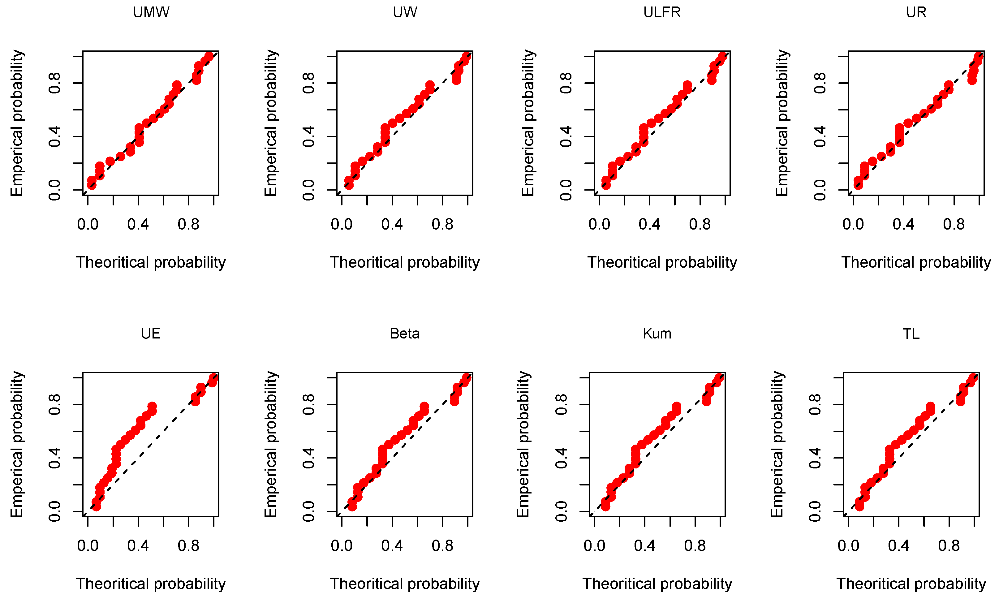
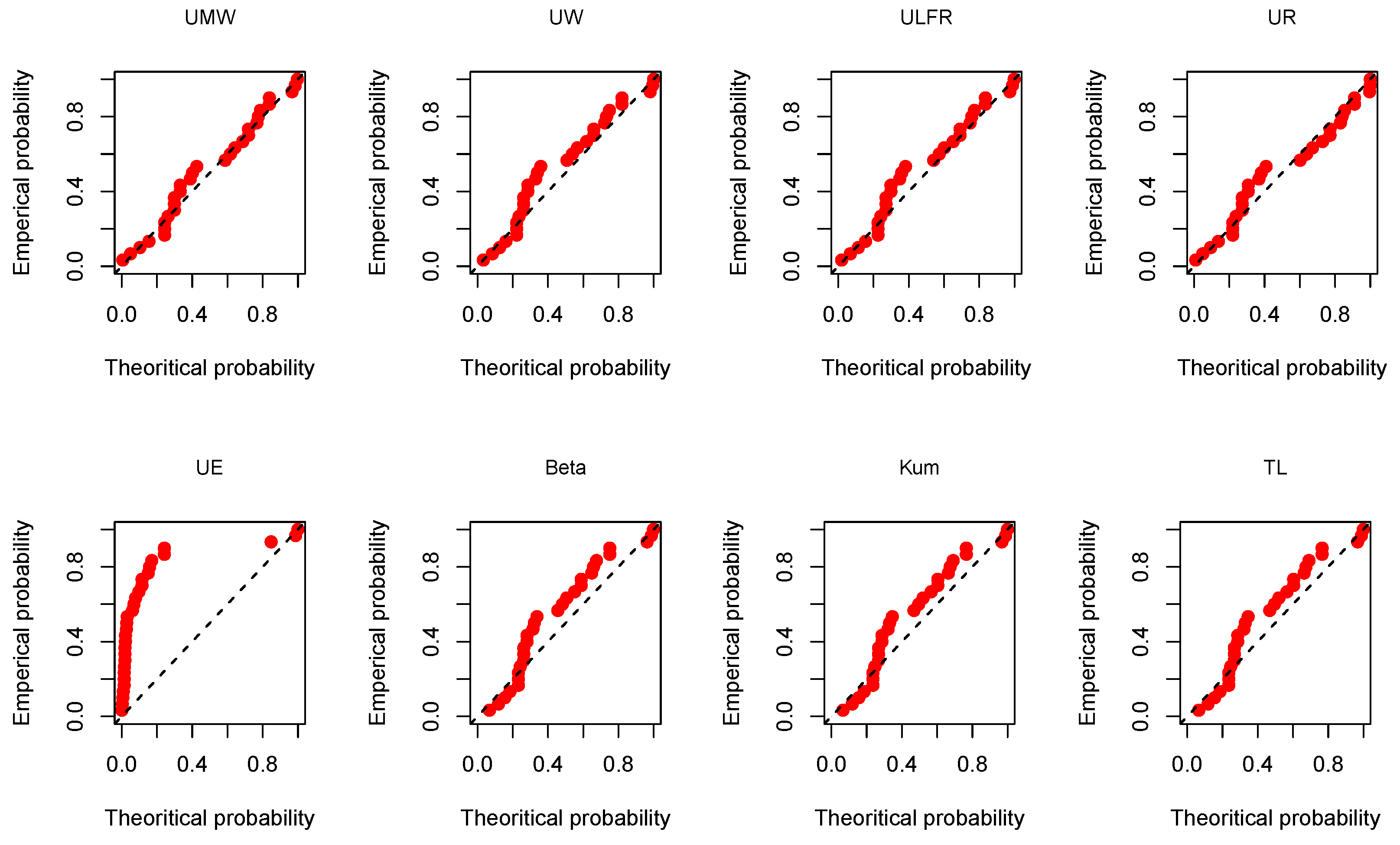
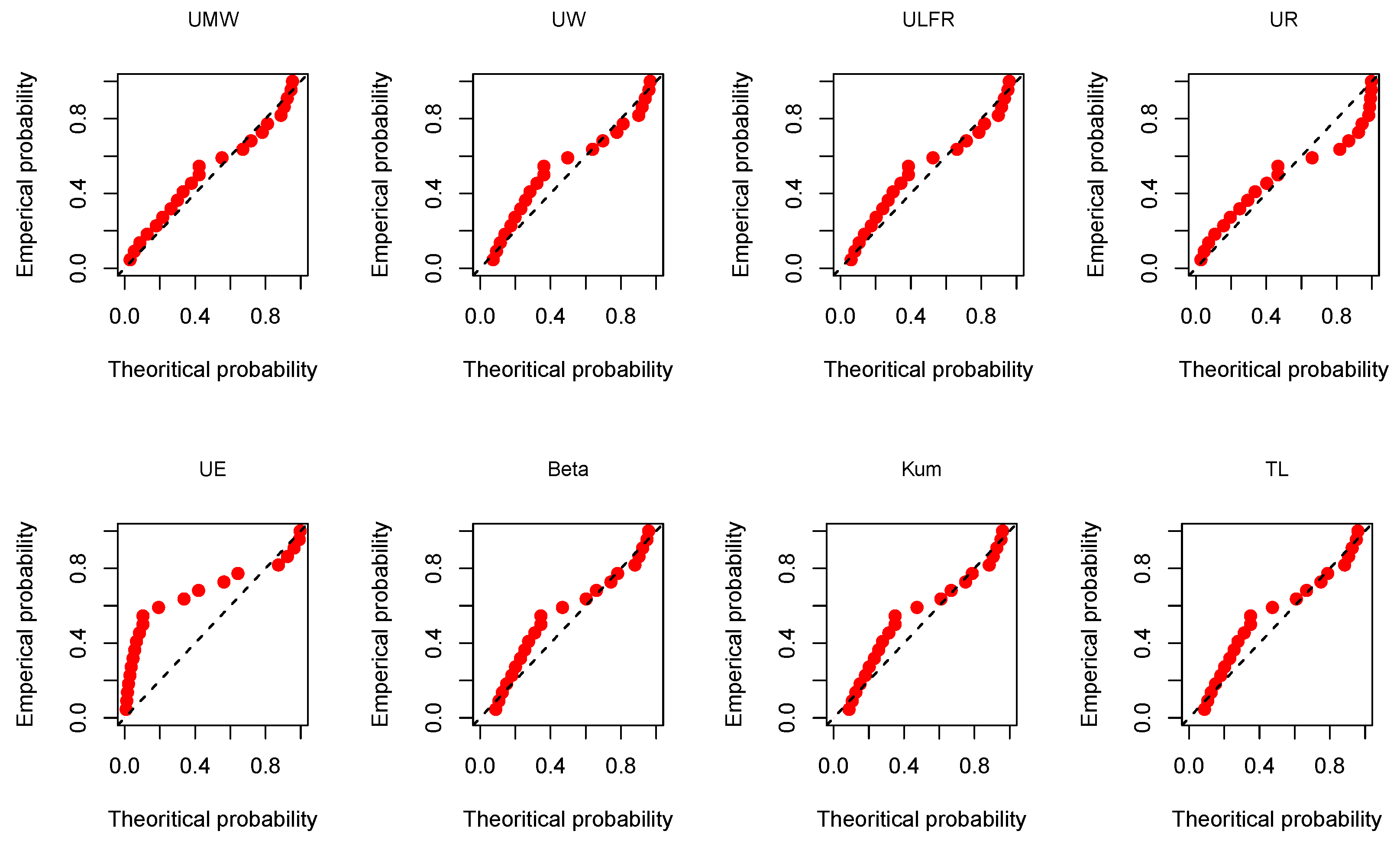
P-P Plots for Model Fit Assessment: Figure 11, Figure 12 and Figure 13 illustrate

• P-P plots for the UMW distribution and the competing distributions.
• Close adherence of the P-P plots, for UMW, to the 45-degree line, indicating excellent agreement between empirical and theoretical probabilities. This further supports the UMW distribution’s superior fit over competing models.

(3)

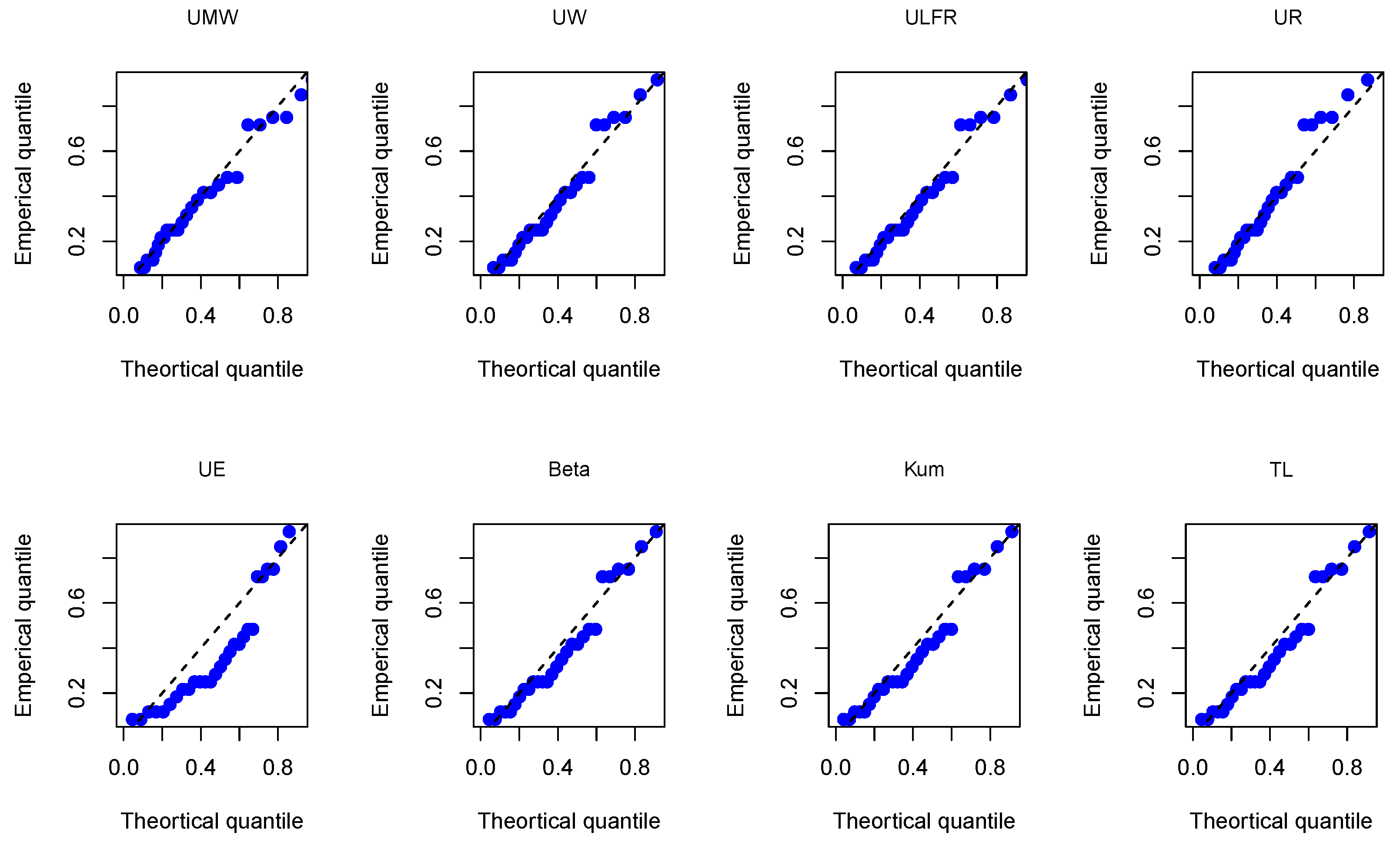
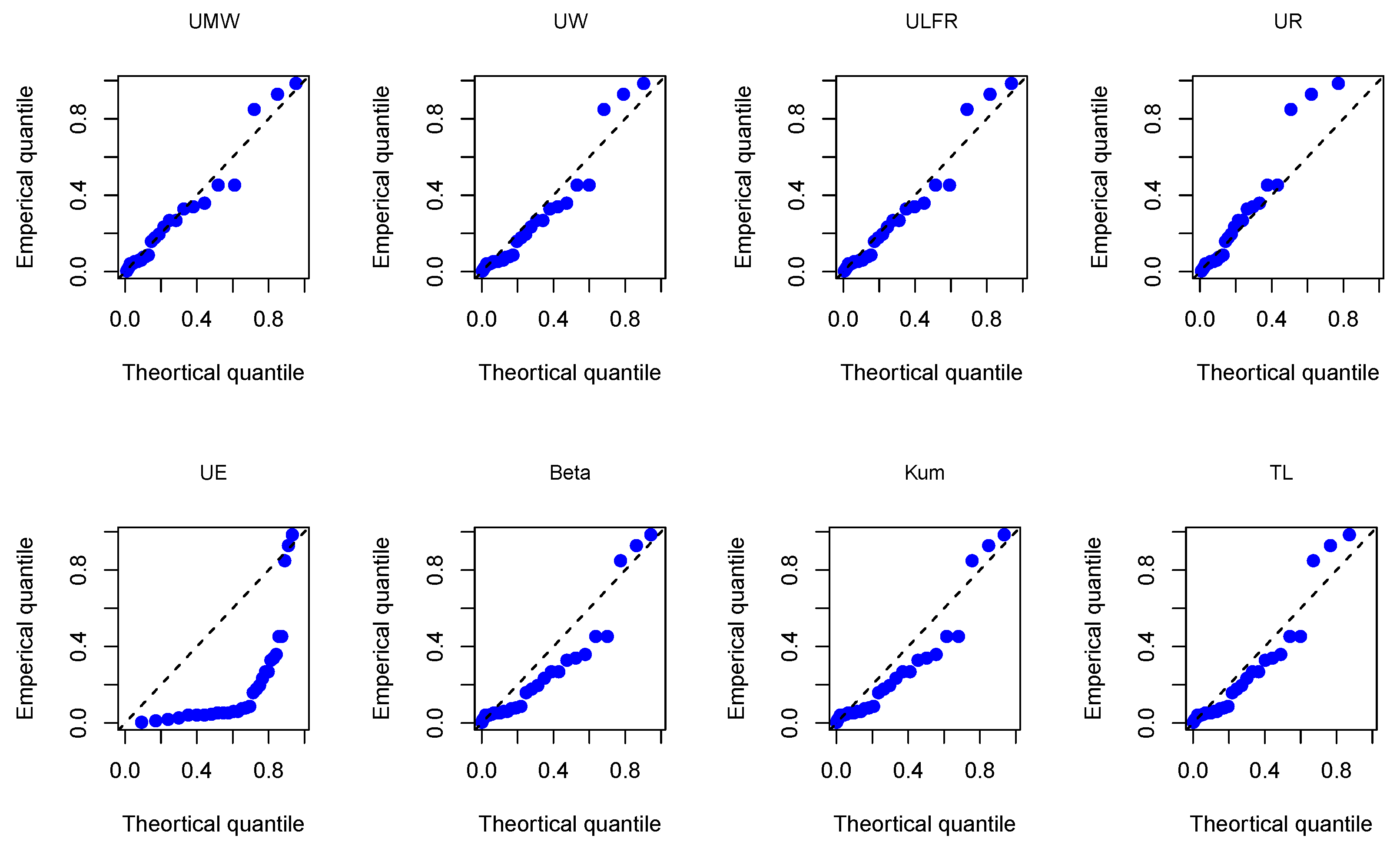
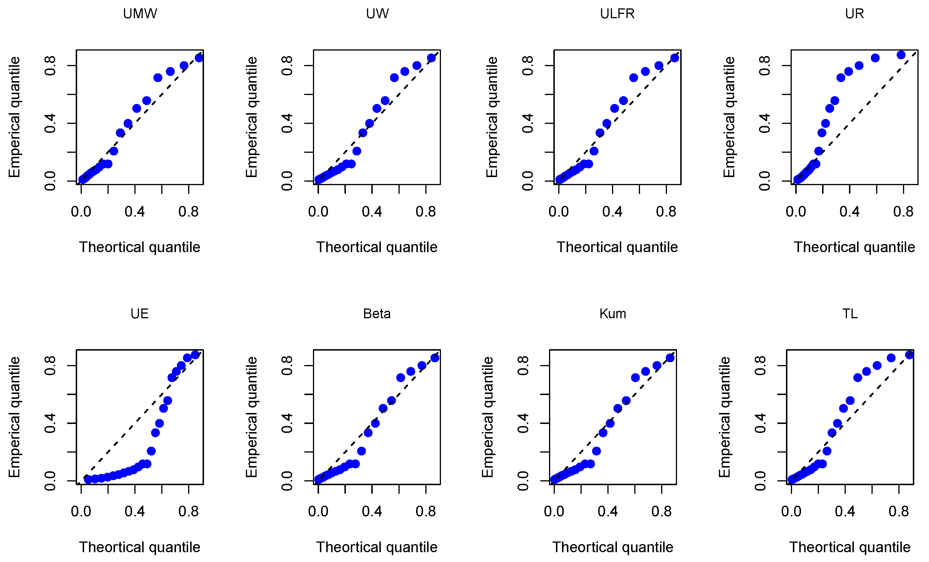
Q-Q Diagnostic Plots: Figure 14, Figure 15 and Figure 16 validate the fit through

• Q-Q plots comparing empirical and theoretical quantiles.
• Near-perfect alignment of data points with the reference line, reinforcing the UMW distribution’s robustness in capturing the empirical data structure.

(4)

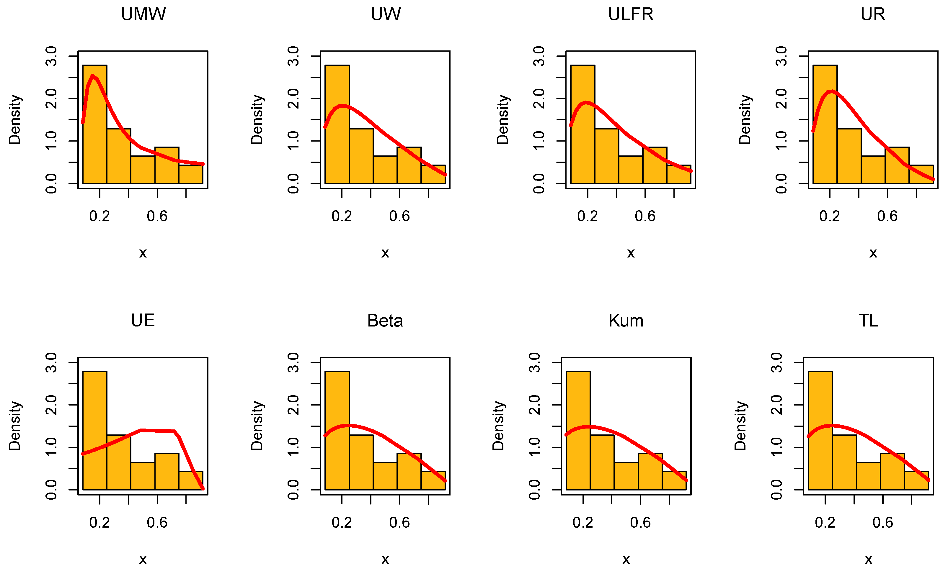
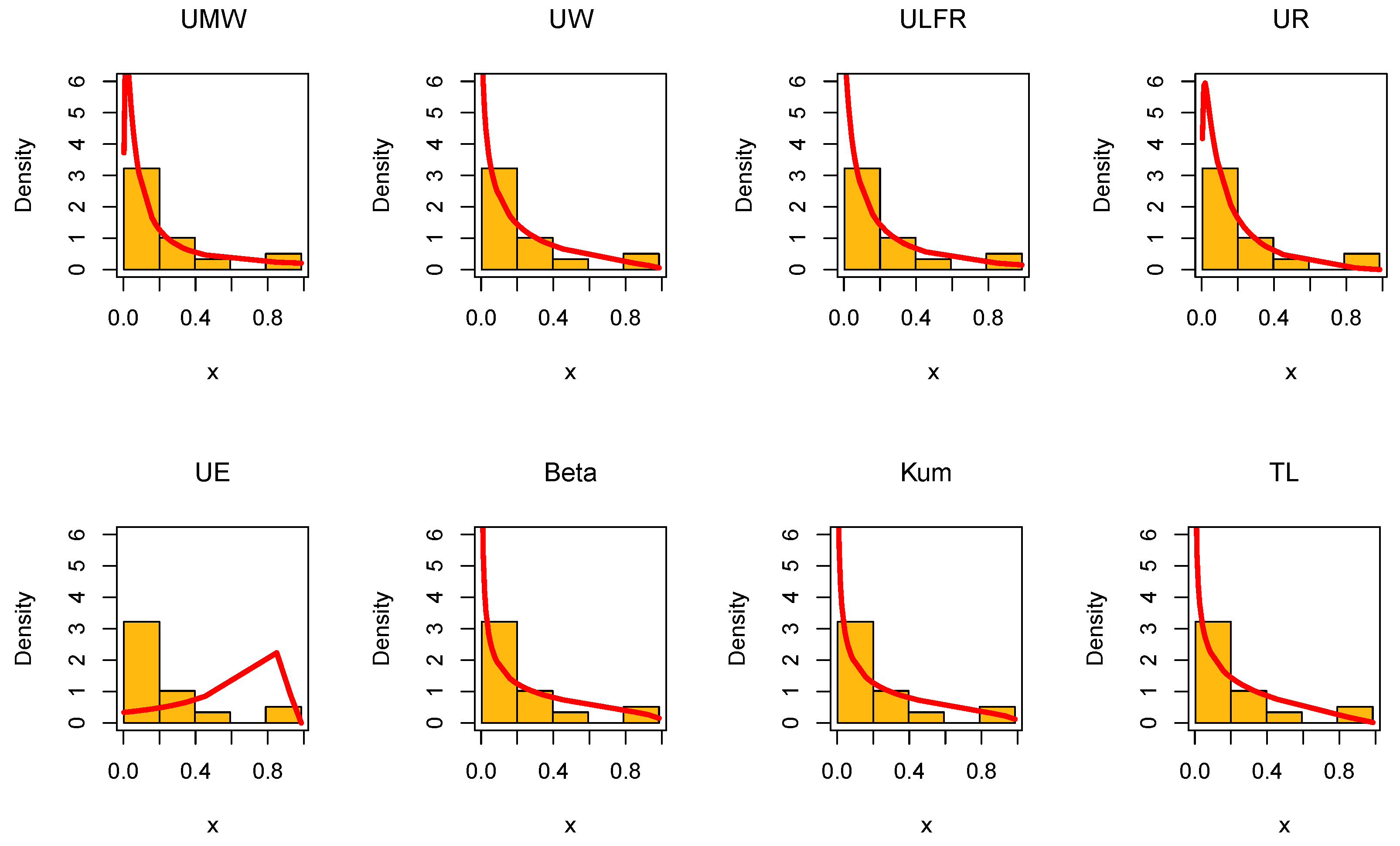
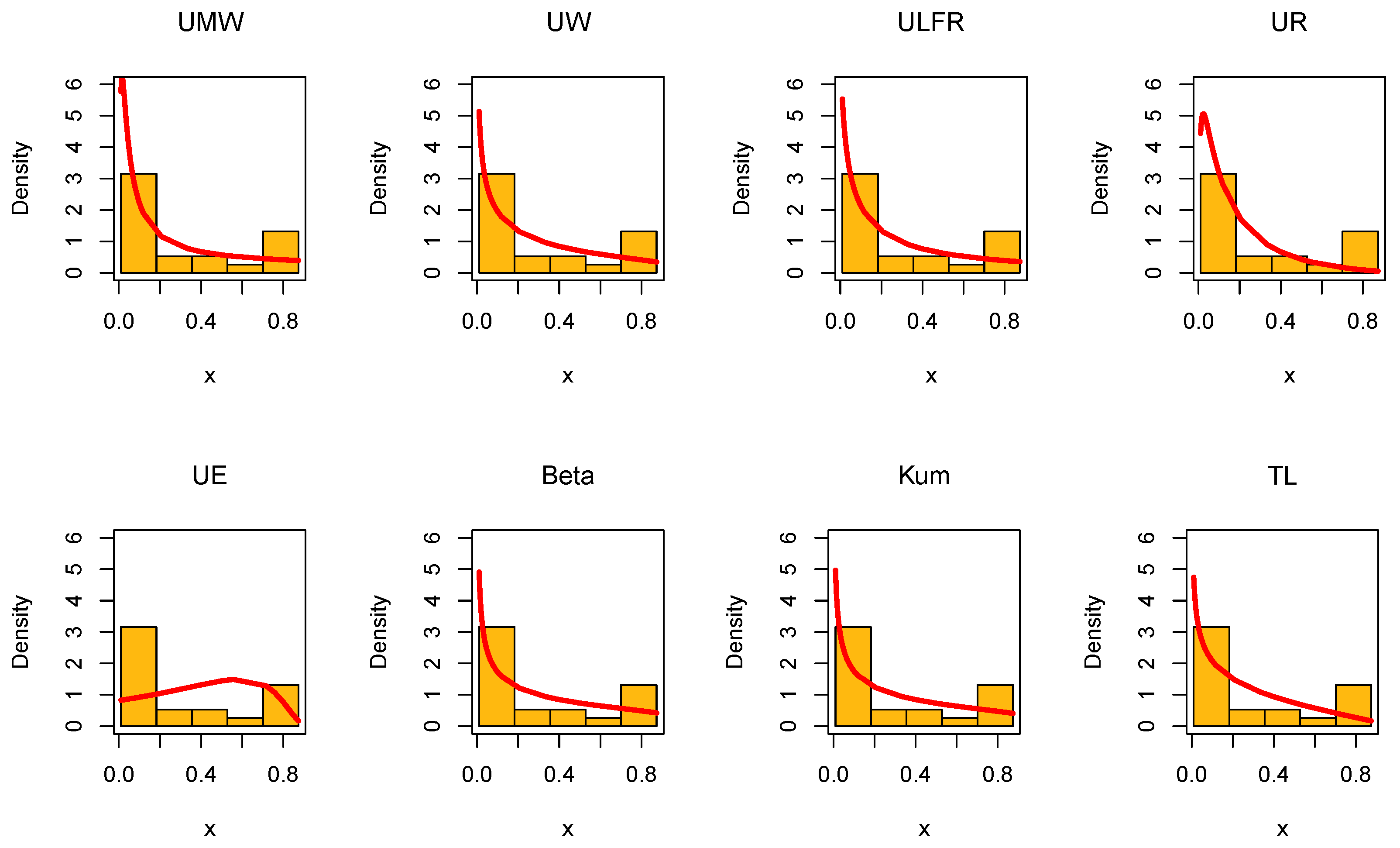
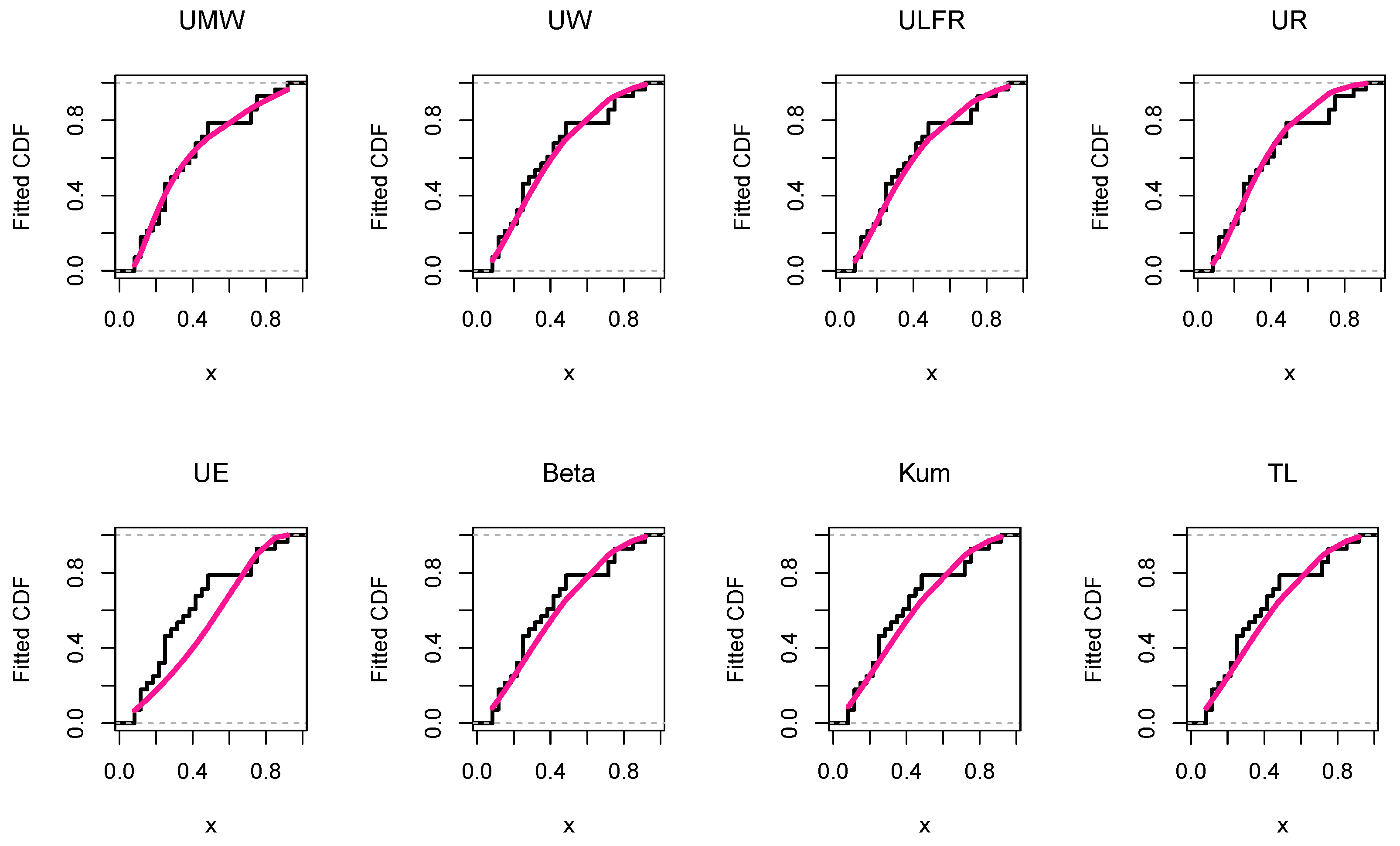
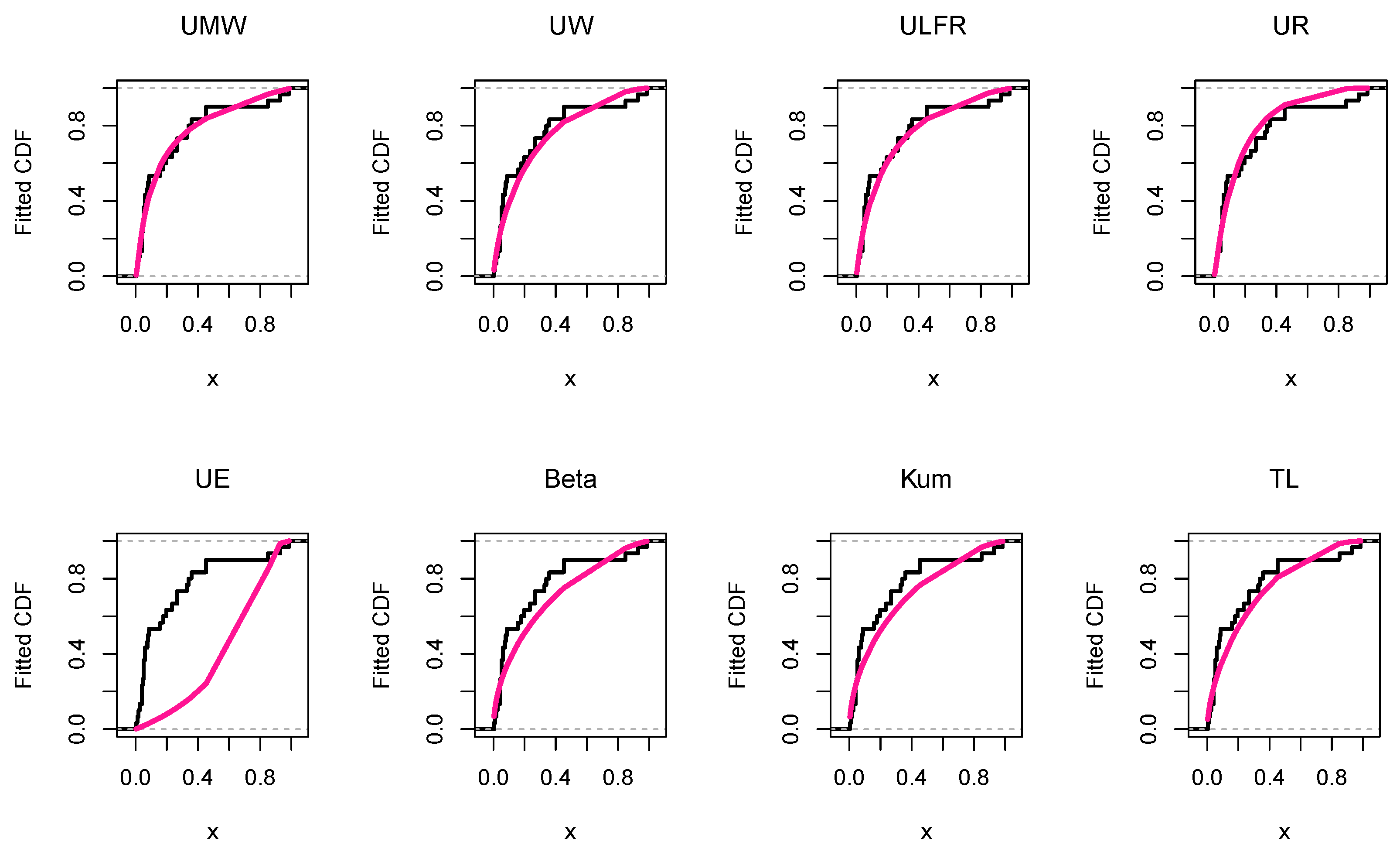
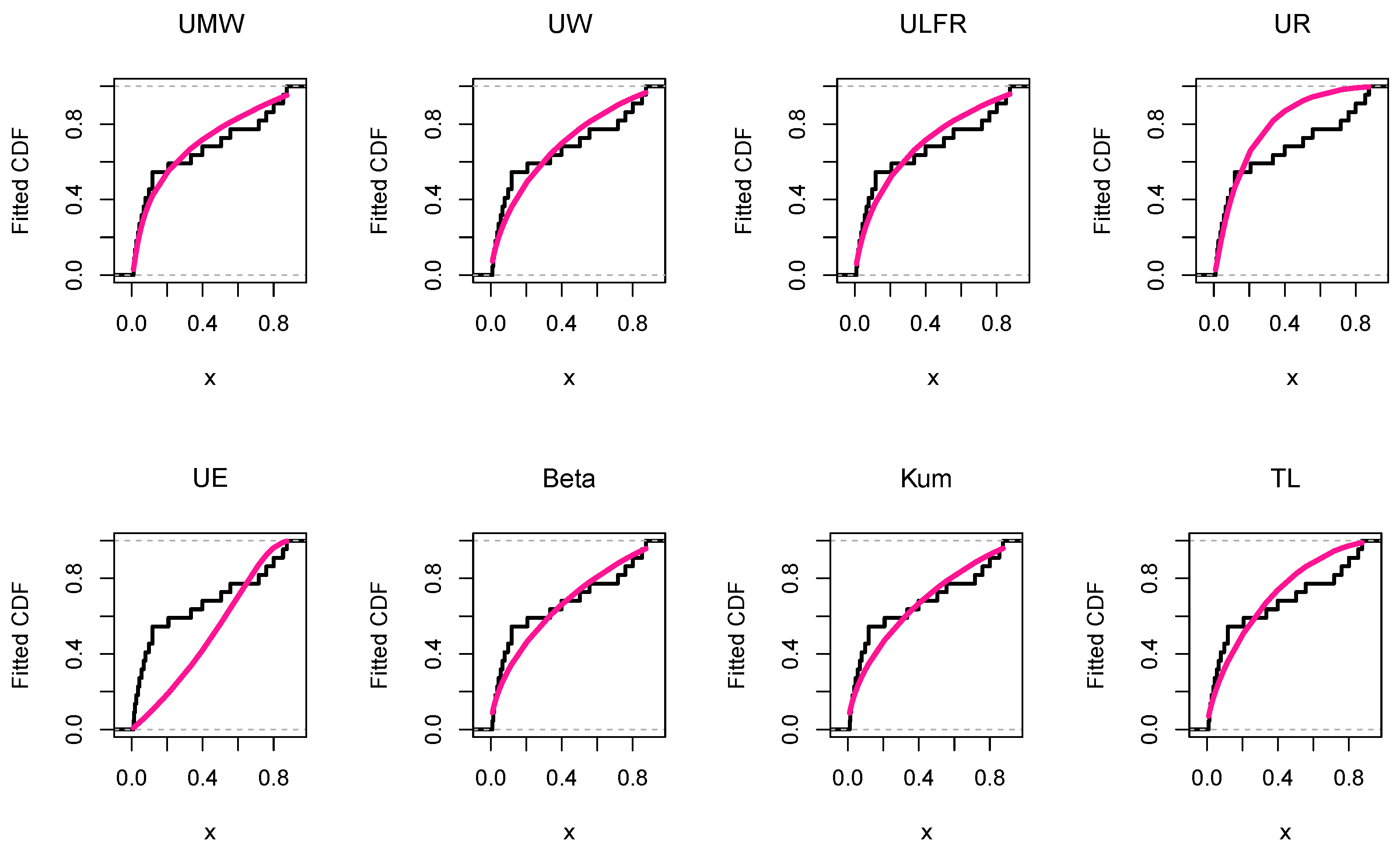
Goodness-of-Fit Visualizations: Figure 17, Figure 18 and Figure 19 and Figure 20, Figure 21 and Figure 22 depict

• Histograms of the data sets overlaid with the fitted UMW density function.
• Empirical versus estimated CDFs, highlighting the UMW model’s accuracy in replicating the observed data trends.

Collectively, the graphical diagnostics, including parameter estimation plots, P–P and Q–Q plots, and distributional visualizations, consistently support the suitability of the UMW distribution for modeling all three real data sets.

For further comparisons between the UMW model and its sub-models, as well as the ULFR model and its sub-models, we utilize the likelihood ratio test statistic, defined as

$$\Lambda =2\left({\mathcal{L}}_{\mathrm{Full}}-{\mathcal{L}}_{\mathrm{Sub}}\right)\sim {\chi }_{df}^2$$

where ${\mathcal{L}}_{\mathrm{Full}}$ and ${\mathcal{L}}_{\mathrm{Sub}}$ are the log-likelihood functions evaluated at the maximum likelihood estimates (MLEs) of the parameters for the full and sub-model, respectively, and df is the difference in the number of parameters between the two models.

Table 14. Testing of hypothesis results.

Full	Sub	df	Data I		Data II		Data III
Model	Model		$\mathbf{\Lambda }$	p-Value	$\mathbf{\Lambda }$	p-Value	$\mathbf{\Lambda }$	p-Value
UMW	UW	1	2.5116	0.11301	6.3526	0.0117	4.7204	0.0298
	ULFR	1	1.7122	0.1907	1.896	0.1685	3.2618	0.0709
	UR	2	3.6688	0.15971	11.1912	0.0037	13.6	0.0011
	UE	2	16.4204	0.00027	108.6044	0.0000	25.223	0.0000
ULFR	UR	1	1.9566	0.16188	9.2952	0.0023	10.3382	0.0013
	UE	1	14.7082	0.00013	106.7084	0.00000	21.9612	0.0000

presents the values of the likelihood ratio test statistic and corresponding p-values across all tested hypotheses, based on the three data sets. From the results, we observe the following:

• Data I: Although the UMW model provides a better fit compared to the UW, ULFR, and UR sub-models, none of these sub-models can be rejected at conventional significance levels. Notably, the UE model is significantly rejected in favor of both UMW and ULFR.
• Data II: All sub-models are significantly rejected compared to UMW, except for ULFR and UR, which do not show significant differences. Additionally, UE is significantly rejected in favor of ULFR.
• Data III: All sub-models are significantly rejected in favor of UMW at significance levels corresponding to p-values less than 0.07, and UR and UE are also significantly rejected in favor of ULFR.

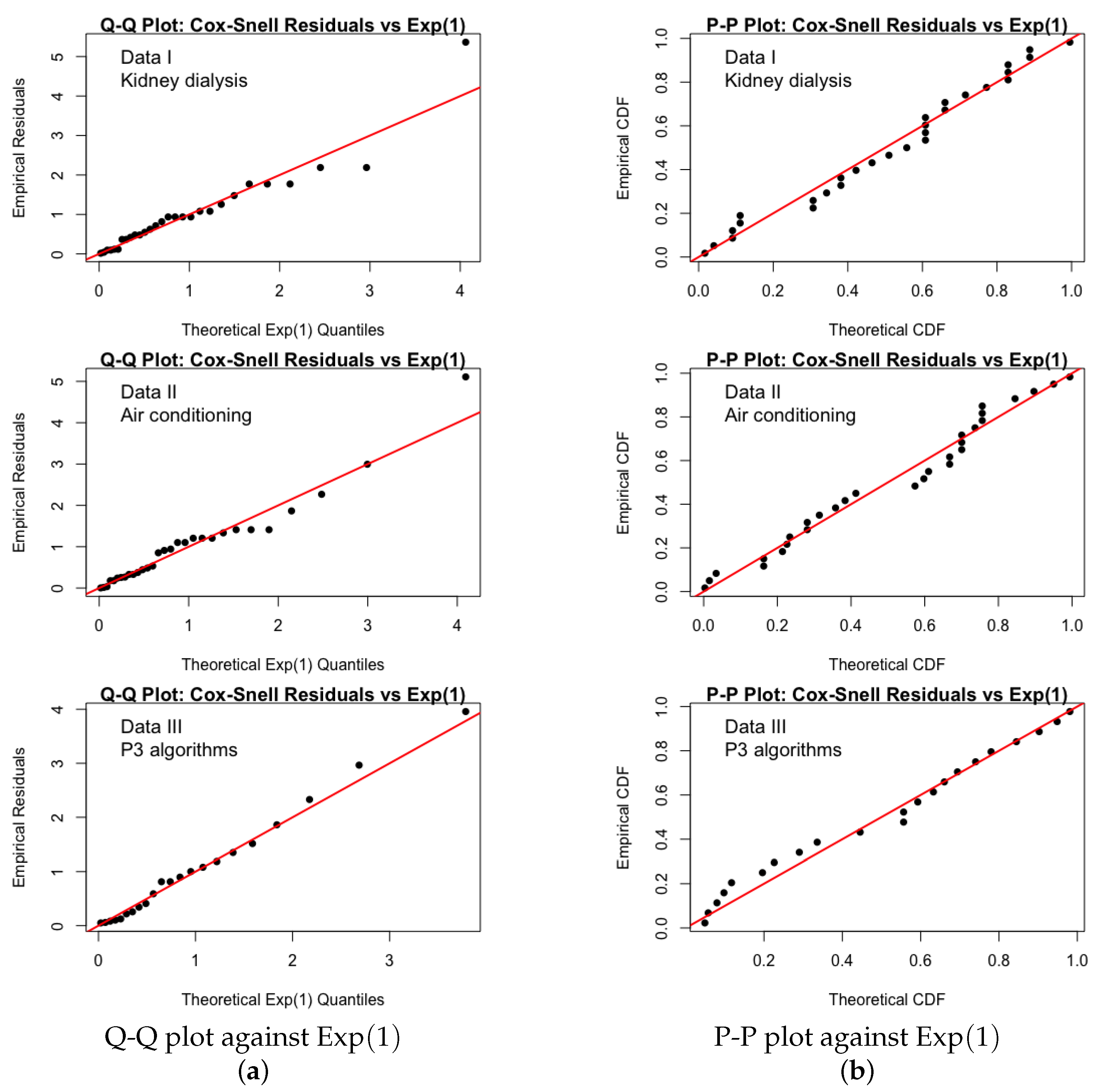
Finally, to assess the adequacy of the proposed UMW distribution in modeling the three lifetime data sets, we employ Cox–Snell residuals [19], a standard diagnostic tool in lifetime analysis. For a correctly specified model, these residuals are expected to follow a standard exponential distribution, i.e., $\mathrm{Exp}\left(1\right)$. The Cox–Snell residual for the i-th observation is defined as

$$r_i=-log\widehat{S}(y_i;\widehat{\mathit{\theta }}),$$

(17)

where $\widehat{S}(y_i;\widehat{\mathit{\theta }})$ is the fitted survival function evaluated at the observed data point $y_i$ using the MLE $\widehat{\mathit{\theta }}$ of the parameter vector.

The validation is performed graphically using Q-Q and P-P plots of the residuals against the theoretical $\mathrm{Exp}\left(1\right)$ distribution. We provide those plots for the three real data sets, as shown in Figure 23.

The collective evidence from both diagnostic plots indicates that the Cox–Snell residuals for the UMW model conform well to the $\mathrm{Exp}\left(1\right)$ distribution for the three data sets. While no model is perfect, the minor deviations in the extreme upper tail of the Q-Q plot, for data I, are not substantial enough to invalidate the model. Therefore, we conclude that the UMW distribution provides an adequate and reasonable fit to the three data sets.

7. Concluding Remarks

This paper presents the Unit-Modified Weibull (UMW) distribution, a new three-parameter model defined on the unit interval $(0, 1)$ for analyzing proportional and fractional data. Developed by transforming the Modified Weibull distribution, the UMW effectively captures diverse hazard rate shapes, including increasing, decreasing, bathtub, and unimodal forms, making it especially useful for modeling bounded data in fields like engineering, medicine, and economics.

We derived the key statistical properties of the distribution and estimated its parameters using the maximum likelihood method. Simulation studies confirmed that the estimators are consistent and reliable across various sample sizes. The model’s practical utility was illustrated through three real-data applications, where it demonstrated better fit than many established unit distributions.

The UMW distribution opens up several avenues for future work, including Bayesian approaches, regression modeling, and more complex reliability applications. Its flexibility and performance suggest it will be a valuable tool for researchers and practitioners working with unit-interval data.

References

1. Consul, P.C.; Jain, G.C. On the log-gamma distribution and its properties. Stat. Hefte 1971, 12, 100–106. [Google Scholar] [CrossRef]
2. Gómez-Déniz, E.; Sordo, M.A.; Calderín-Ojeda, E. The Log–Lindley distribution as an alternative to the beta regression model with applications in insurance. Insur. Math. Econ. 2014, 54, 49–57. [Google Scholar] [CrossRef]
3. Condino, F.; Domma, F. A new distribution function with bounded support: The reflected generalized Topp-Leone power series distribution. Metron 2017, 75, 51–68. [Google Scholar] [CrossRef]
4. Mazucheli, J.; Menezes, A.F.B.; Ghitany, M.E. The unit-Weibull distribution and associated inference. J. Appl. Probab. Stat. 2018, 13, 1–22. [Google Scholar]
5. Altun, E.; Hamedani, G.G. The log-xgamma distribution with inference and application. J. Société Française Stat. 2018, 159, 40–55. [Google Scholar]
6. Mazucheli, J.; Menezes, A.F.; Dey, S. Unit-Gompertz distribution with applications. Statistica 2019, 79, 25–43. [Google Scholar]
7. Ribeiro-Reis, L.D. Unit log-logistic distribution and unit log-logistic regression model. J. Indian Soc. Probab. Stat. 2021, 22, 375–388. [Google Scholar] [CrossRef]
8. Korkmaz, M.Ç.; Chesneau, C. On the unit Burr-XII distribution with the quantile regression modeling and applications. Comput. Appl. Math. 2021, 40, 29. [Google Scholar] [CrossRef]
9. Haq, M.A.U.; Hashmi, S.; Aidi, K.; Ramos, P.L.; Louzada, F. Unit modified Burr-III distribution: Estimation, characterizations and validation test. Ann. Data Sci. 2023, 10, 415–440. [Google Scholar] [CrossRef]
10. Al-Omari, A.I.; Alanzi, A.R.; Alshqaq, S.S. The unit two parameters Mirra distribution: Reliability analysis, properties, estimation and applications. Alex. Eng. J. 2024, 92, 238–253. [Google Scholar] [CrossRef]
11. Sarhan, A.M. Unit-Chen distribution and its quantile regression model with applications. Sci. Afr. 2025, 27, e02555. [Google Scholar] [CrossRef]
12. Sarhan, A.M.; Sobh, M.E. Unit exponentiated weibull model with applications. Sci. Afr. 2025, 27, e02606. [Google Scholar] [CrossRef]
13. Sarhan, A.M.; Zaindin, M. Modified Weibull distribution. Appl. Sci. 2009, 11, 123–136. [Google Scholar]
14. Bakouch, H.S.; Hussain, T.; Tošić, M.; Stojanović, V.S.; Qarmalah, N. Unit exponential probability distribution: Characterization and applications in environmental and engineering data modeling. Mathematics 2023, 11, 4207. [Google Scholar] [CrossRef]
15. Bantan, R.A.; Chesneau, C.; Jamal, F.; Elgarhy, M.; Tahir, M.H.; Ali, A.; Anam, S. Some new facts about the unit-Rayleigh distribution with applications. Mathematics 2020, 8, 1954. [Google Scholar] [CrossRef]
16. Alotaibi, N.; Hashem, A.F.; Elbatal, I.; Alyami, S.A.; Al-Moisheer, A.S.; Elgarhy, M. Inference for a Kavya–Manoharan inverse length biased exponential distribution under progressive-stress model based on progressive type-II censoring. Entropy 2022, 24, 1033. [Google Scholar] [CrossRef] [PubMed]
17. Linhart, H.; Zucchini, W. Model Selection; Wiley: New York, NY, USA, 1986. [Google Scholar]
18. Caramanis, M.; Stremel, J.; Fleck, W.; Daniel, S. Probabilistic production costing: An investigation of alternative algorithms. Int. J. Electr. Power Energy Syst. 1983, 5, 75–86. [Google Scholar] [CrossRef]
19. Cox, D.R.; Snell, E.J. A general definition of residuals. J. R. Stat. Soc. Ser. (Methodol.) 1968, 30, 248–275. [Google Scholar] [CrossRef]
Figure 1. The PDF and HRF of UMW distribution for different values of α , β , γ .
Stats 08 00081 g001
Figure 2. The MSE of the MLE obtained via simulation, with true parameter values α = 0.5 , β = 0.5 , and γ = 0.8 .
Stats 08 00081 g002
Figure 3. The MSE of the MLE obtained via simulation, with true parameter values α = 0.8 , β = 1 , and γ = 1.5 .
Stats 08 00081 g003
Figure 4. The MSE of the MLE obtained via simulation, with true parameter values α = 1.2 , β = 1.5 , and γ = 3 .
Stats 08 00081 g004
Figure 5. The MSE of the MLE obtained via simulation, with true parameter values α = 1.2 , β = 0.5 , and γ = 0.2 .
Stats 08 00081 g005
Figure 6. TTT plot for the three data sets.
Stats 08 00081 g006
Figure 7. The violin plots for the three data sets.
Stats 08 00081 g007
Figure 8. Profile likelihood functions vs. the UMW’s parameters for the kidney dialysis data.
Stats 08 00081 g008
Figure 9. Profile likelihood functions vs. the UMW’s parameters for air conditioning data.
Stats 08 00081 g009
Figure 10. Profile likelihood functions vs. the UMW’s parameters for P3 algorithm data.
Stats 08 00081 g010
Figure 11. The P-P plots for the kidney dialysis data using the eight competitive models.
Stats 08 00081 g011
Figure 12. The P-P plots for the air conditioning data using all used models.
Stats 08 00081 g012
Figure 13. The P-P plots for the P3 algorithm data using all models.
Stats 08 00081 g013
Figure 14. The Q-Q plots for the kidney dialysis data using all models.
Stats 08 00081 g014
Figure 15. The Q-Q plots for the air conditioning data using all models.
Stats 08 00081 g015
Figure 16. The Q-Q plots for the P3 algorithm data using all models.
Stats 08 00081 g016
Figure 17. Histogram of the kidney dialysis data with the fitted PDFs of all compared models.
Stats 08 00081 g017
Figure 18. Histogram of the air conditioning data with the fitted PDFs of all compared models.
Stats 08 00081 g018
Figure 19. Histogram of the P3 algorithm data with the fitted PDFs of all compared models.
Stats 08 00081 g019
Figure 20. The empirical and fitted CDF for the kidney dialysis data using the competitive models.
Stats 08 00081 g020
Figure 21. The empirical and fitted CDF for the air conditioning data using the competitive models.
Stats 08 00081 g021
Figure 22. The empirical and fitted CDF for the P3 algorithm data using the competitive models.
Stats 08 00081 g022
Figure 23. (a) Q-Q plots of Cox–Snell residuals against the theoretical Exp(1) distribution for the three data sets. (b) P-P plots of the empirical CDF of the residuals against the theoretical Exp(1) CDF.
Stats 08 00081 g023