Communication

On the Appropriateness of Fixed Correlation Assumptions in Repeated-Measures Meta-Analysis: A Monte Carlo Assessment

by
Vasileios Papadopoulos
Laboratory of Anatomy, Department of Medicine, Democritus University of Thrace, GR-68100 Alexandroupolis, Greece
Stats 2025, 8(3), 72; https://doi.org/10.3390/stats8030072
Submission received: 19 June 2025 / Revised: 8 August 2025 / Accepted: 10 August 2025 / Published: 13 August 2025

Abstract

In repeated-measures meta-analyses, raw data are often unavailable, preventing the calculation of the correlation coefficient r between pre- and post-intervention values. As a workaround, many researchers adopt a heuristic approximation of r = 0.7. However, this value lacks rigorous mathematical justification and may introduce bias into variance estimates of pre/post-differences. We employed Monte Carlo simulations (n = 500,000 per scenario) in Fisher z-space to examine the distribution of the standard deviation of pre-/post-differences (σD) under varying assumptions of r and its uncertainty (σr). Scenarios included r = 0.5, 0.6, 0.707, 0.75, and 0.8, each tested across three levels of variance (σr = 0.05, 0.1, and 0.15). The approximation of r = 0.75 resulted in a balanced estimate of σD, corresponding to a “midway” variance attenuation due to paired data. This value more accurately offsets the deficit caused by assuming a correlation, compared to the traditional value of 0.7. While the r = 0.7 heuristic remains widely used, our results support the use of r = 0.75 as a more mathematically neutral and empirically defensible alternative in repeated-measures meta-analyses lacking raw data.

1. Introduction

Many authors aiming to conduct a meta-analysis involving paired data on continuous numerical variables typically use the arithmetic difference between pre- and post-intervention measurements as the effect size. However, in doing so, they often lack raw data, which forces them to rely solely on aggregated statistics (i.e., pre- and post-means and their corresponding standard deviations). This reliance complicates the direct and accurate estimation of the mean of the pre/post-differences—and, more critically, its variability. The main reason is that in many individual studies, the correlation coefficient r between pre- and post-values either is not reported or cannot be computed, making it impossible to use this parameter in indirect variance estimation. Some statistical software, such as UNISTAT, assumes a correlation of 0.5 by default, in case this information is not readily available [1]. However, many authors—including the present author—commonly adopt an arbitrary value of r = 0.7 [2,3,4,5,6,7], an approach based on earlier work beginning with Rosenthal [8]. This communication article aims to examine whether this approach is empirically defensible, whether there is a mathematically valid rationale for it, and the consequences of its use. Finally, this article explores potentially sound alternatives to the already proposed fixed-r assumptions.

2. Materials and Methods

Let μpre and μpost be the mean of the values between two timepoints in a repeated-measures design study, i.e., before and after the intervention (pre- and post-values, respectively) and r be the Pearson’s correlation coefficient between pre- and post-values. Additionally, let σpre and σpost be the standard deviations corresponding to μpre and μpost, respectively.
The mean of the pre-/post-differences μD is given by the formula μD = μpostμpre. Of note, the standard deviation σD of μD is given by the formula σD = (σpre2 + σpost2 − 2preσpost)1/2.
To approximate the expected σD (℮|σD|), we used Monte Carlo simulations (500,000 per condition) in Fisher z-space, applying the formula z = tanh−1(r) = 1/2ln[(1 + r)/(1 − r)] and back-transforming to r ∈ (−1,1) using r = tanh(z). While the Central Limit Theorem (CLT) does not imply normality for r itself, it motivates the approximation of the Fisher z-transformation of r as approximately normal in large samples with variance 1/(n − 3) for sample size n. When standardized normal distribution is implemented, σD = [2σ2(1 − r)]1/2 becomes σD = (1 − r)1/2 [9].
All simulations were performed using R version 4.5.1 (R Core Team, 2024); the complete R code is provided as Appendix A.
ChatGPT 4 was implemented to partly construct the R code and generate Figures 2 and 4.

3. Results

3.1. What Are the Consequences of r Uncertainty?

Let us consider a hypothetical infinite-sample scenario and investigate what happens to the σD when μD is constant and r is a random variable that is distributed normally presenting a mean of 0.5, under the assumption of equal pre-/post-variances (σpre = σpost = σ).
By substituting σpre = σpost = σ into the formula σD = (σpre2 + σpost2 − 2preσpost)1/2, we receive σD = [2σ2(1 − r)]1/2. Thus, the expected σD, ℮|σD|, is given by the formula ℮|σD|= 21/2σ℮|(1 − r)1/2|, where ℮|(1 − r)1/2| is the expected (1 − r)1/2. Note that, despite r being hypothesized to be distributed normally, it must be clipped to [0,1] to be interpretable; therefore, (1 − r)1/2 is not normally distributed. Consequently, ℮|(1 − r)1/2| generally has no closed form but can be approximated numerically or via Taylor expansion, particularly if the distribution of r is tightly concentrated around its mean [10].
Applying second-order Taylor expansion for f(X) = X1/2 = (1 − r)1/2, ℮|f(X)| ≈ f(μX) + 1/2f″(μX)Var(Χ).
By substituting f(X) = (1 − r)1/2, μX = 0.5, Var(Χ) = σX2 = σr2, f(μX) = μX1/2, and f(μX) = −1/4μX−3/2, ℮|(1 − r)1/2| ≈ (0.5)1/2 − 1/8(0.5)−3/2σr2 = (0.5)1/2 − 1/2(0.5)1/2σr2.
Consequently, ℮|σD| = 21/2σ℮|(1 − r)1/2| => ℮|σD| = 21/2σ[(0.5)1/2 − 1/2(0.5)1/2σr2] => ℮|σD|= σ[1 − 1/2σr2].
For a reasonable value of σr, e.g., σr = 0.1, we receive ℮|σD| ≈ σ[1 − 1/2(0.1)2] = 0.995σ. This implies that even considerable uncertainty in r results in a slight inflation of the variability in the pre/post-difference.
In its general form (i.e., for any r), ℮|σD| = 21/2σ{(1 − r)1/2 − 1/[8(1 − r)3/2]σr2}. For ℮|σD|< 0, the Taylor approximation breaks down, yielding negative or undefined results. Solving for ℮|σD|= 0, the critical value for this breakdown is σr(crit) = 23/2(1 − r). A graphical representation of the validity of the Taylor approximation is provided in Figure 1.

3.2. Does the r = 0.7 Heuristic Satisfy the “Midway” Hypothesis for Equal Pre/Post-Variances?

Let us examine the case under the assumption of r = 1/21/2 ≈ 0.707 ≈ 0.7 and the presence of equal pre/post-variances (σpre = σpost = σ).
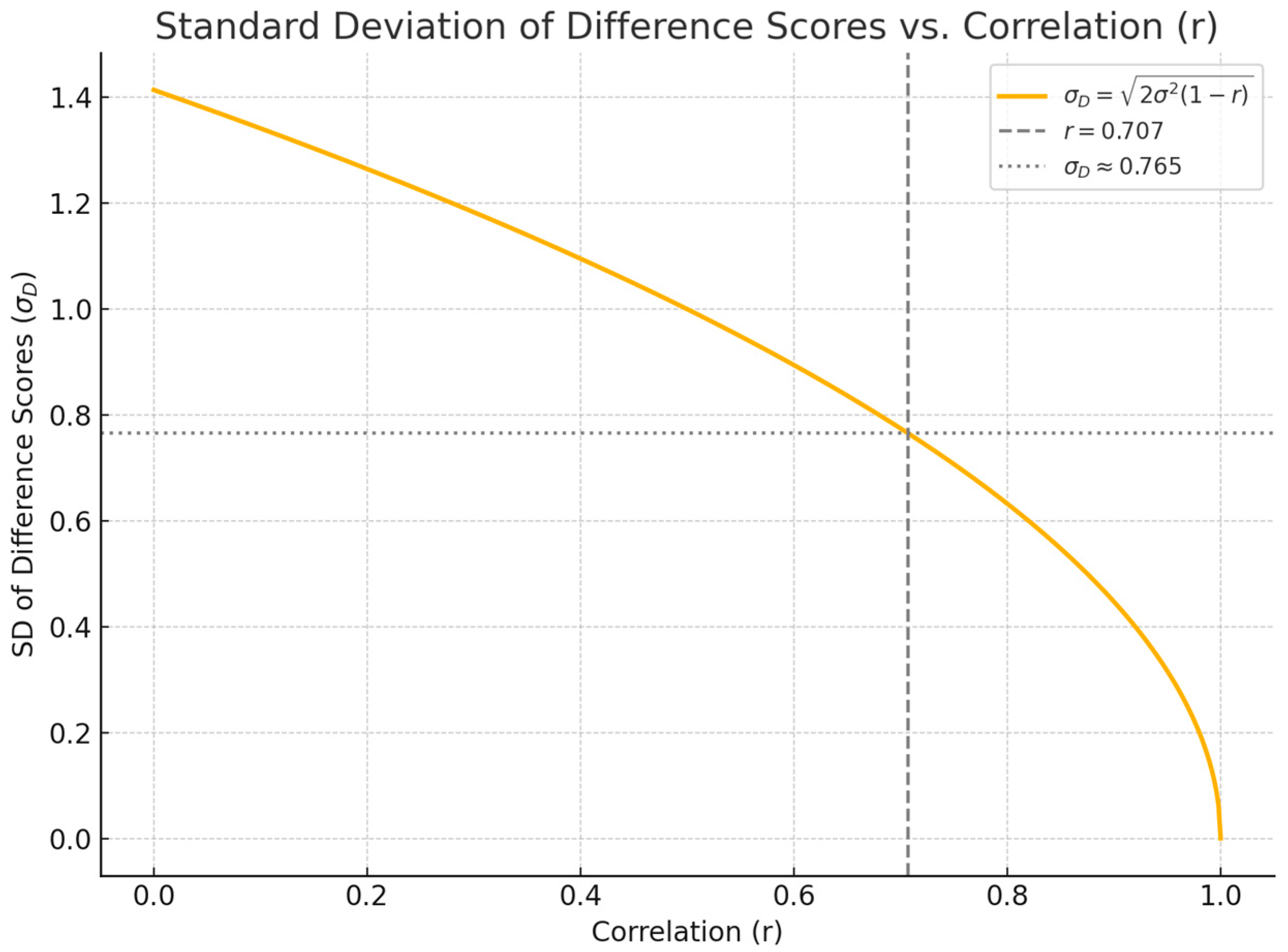
Under these circumstances, the formula σD = (σpre2 + σpost2 − 2preσpost)1/2 would become σD = (2σ2 − 22)1/2 = σ[2(1 − (1/21/2)] ≈ 0.765σ (Figure 2).
The standard deviation of the pre/post-difference is smaller than the standard deviation of the pre- and post-values due to their positive correlation. Of note, assuming r = 1/21/2 ≈ 0.707 helps to counterbalance the over- and underestimation of the true variability in repeated-measures designs; however, this is an arbitrary choice that has no further mathematical documentation.
In detail, in the case of the absence of any correlation (r = 0), the formula σD = (σpre2 + σpost2 − 2preσpost)1/2 gives σD = (21/2)σ ≈ 1.414 σ. Accordingly, when there is an absolute correlation (r = 1), the formula σD = (σpre2 + σpost2 − 2preσpost)1/2 gives σD = 0.
Under these circumstances, a “midway” assumption would have to result in σD ≈ 0.707 σ. Solving σD = (σpre2 + σpost2 − 2preσpost)1/2 for σD ≈ 0.707 σ, under the assumption of equal pre/post-variances (σpre = σpost= σ), we obtain r = 0.75.

3.3. Simulation of Uncertainty of σD to Examine the Feasibility of the Proposed r = 0.75 for Equal Pre/Post-Variances

The above-mentioned theoretical approach to estimate σD has the disadvantage of using a truncated normal distribution for r. This approximation is considered tolerable as σr decreases.
A more accurate approach to estimate σD is the use of 500,000 Monte Carlo simulations per condition in Fisher z-space using the formula z = tanh−1(r) = 1/2ln[(1 + r)/(1 − r)] and back-transforming to r ∈ (−1,1) using r = tanh(z). In this special case, σD = [2σ2(1 − r)]1/2 would become σD = (1 − r)1/2, as σ = 1 for the implemented standardized normal distribution.
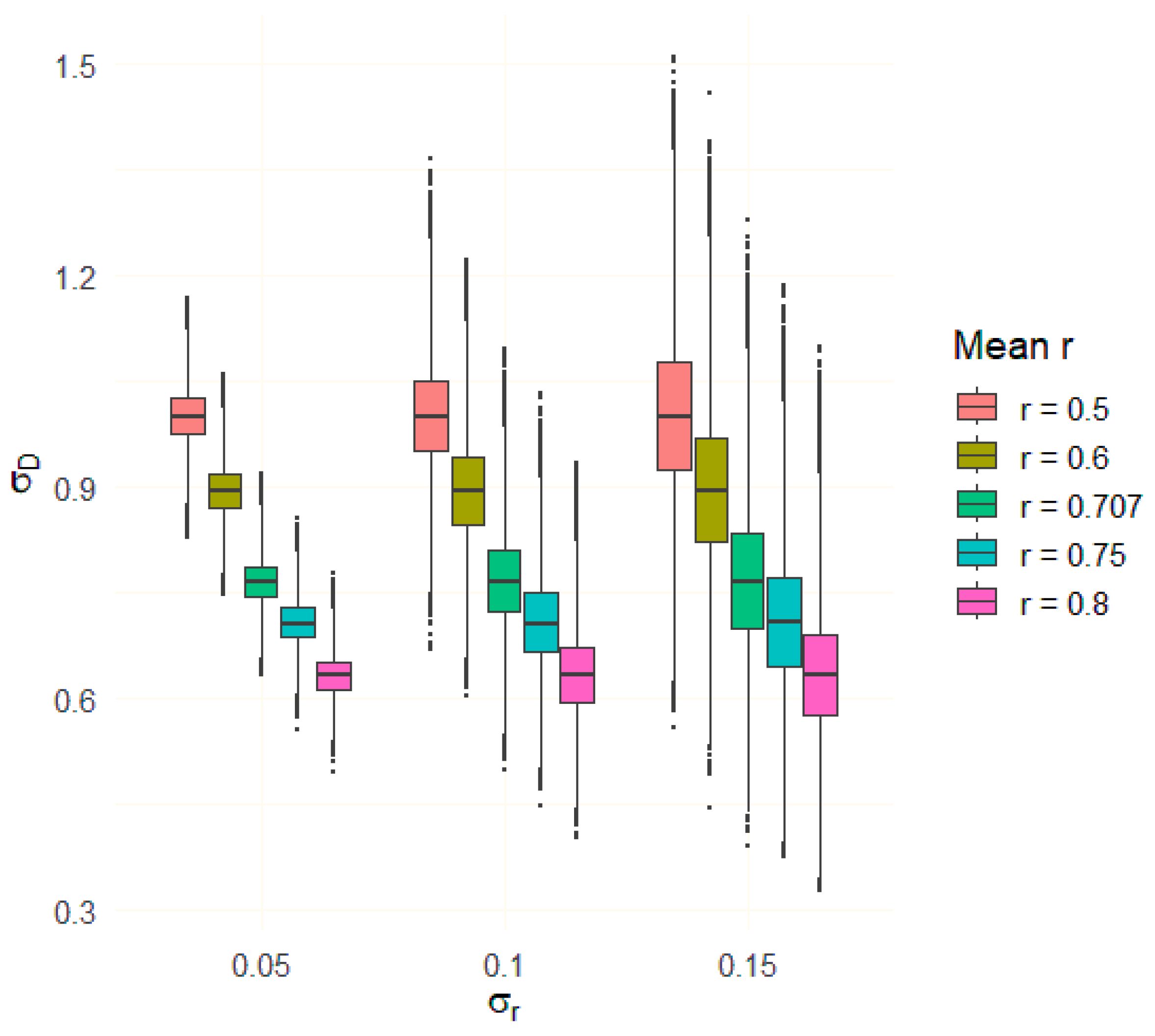
In detail, we used Monte Carlo simulations to analyze five sets of scenarios (targeting r = 0.5, r = 0.6, r = 0.707, r = 0.75, and r = 0.8) to investigate ℮|σD|. For each set of scenarios, we examined three levels of uncertainty of σ (σr): 0.05, 0.1, and 0.15. As expected, increasing the correlation reduces variability in the pre/post-differences. A box-and-whisker plot showing the distribution of σD for all considered levels of uncertainty of σr is depicted in Figure 3; note that for r = 0.75 and σr = 0.1, ℮|σD| is close to the theoretical approximation of 0.707σ.
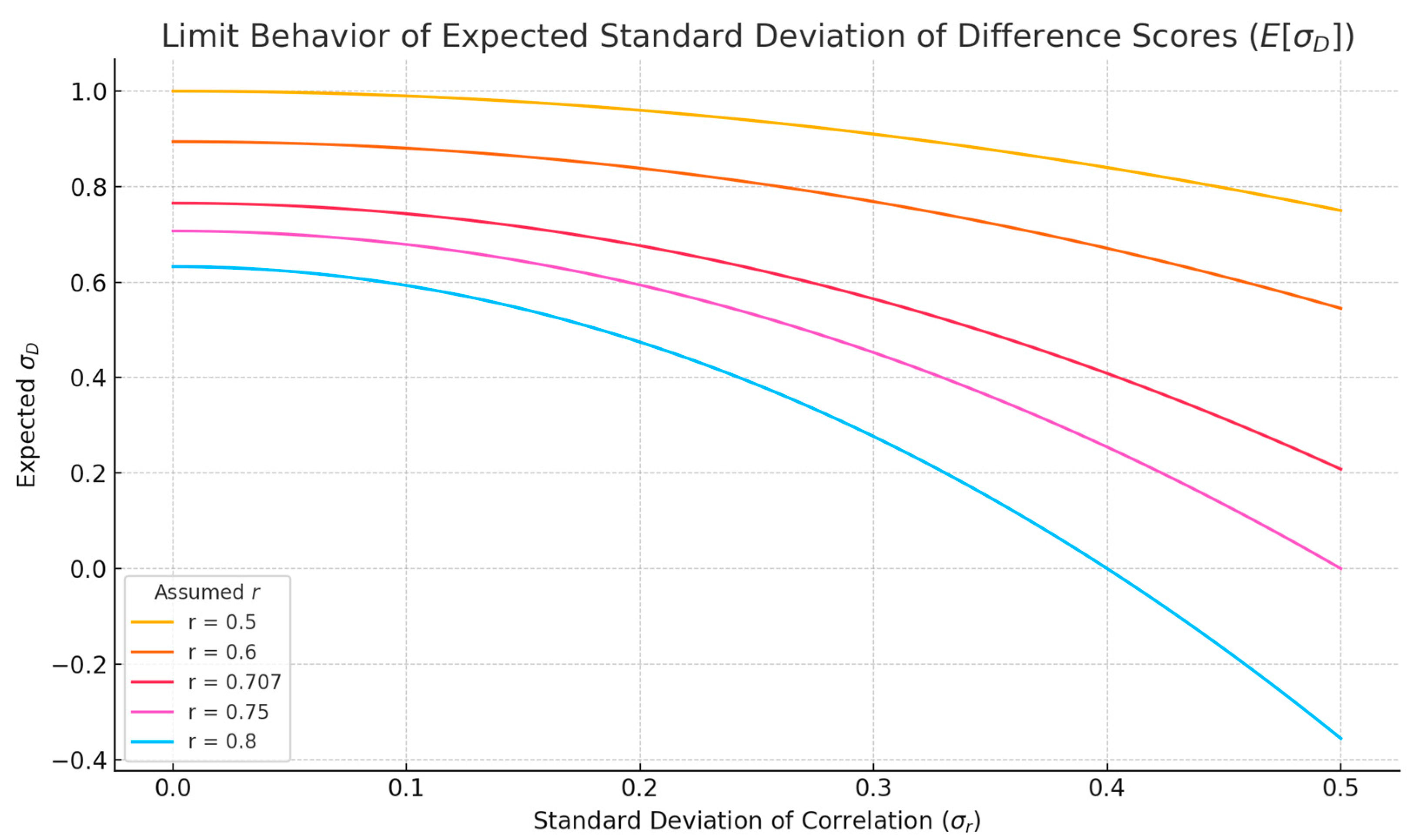
Furthermore, Figure 4 demonstrates the limit behavior of ℮|σD| versus σr2; for reasonable values of σr2 (i.e., ≤0.2), ℮|σD| is slightly affected. Of note, for σD2 < 0, the Taylor expansion breaks down, yielding negative or imaginary results that are no longer valid.

3.4. The “Midway” Hypothesis for Proposed r Under Unequal Pre/Post-Variances

Let us examine the case of unequal pre/post-variances (σpreσpost = σ), where σpre/σpost = b ≠ 1. In that case, σD = σpost (b2 + 1 − 2rb)1/2. Of note, σD is minimum for r = 1 (σD(min) = σpost |b − 1|) and maximum for r = 0 (σD(max) = σpost (b2 + 1)1/2). As such, the “midway” assumption would be satisfied for σpost = (σD(min) + σD(max))/2 = [|b − 1| + (b2 + 1)1/2]/2.
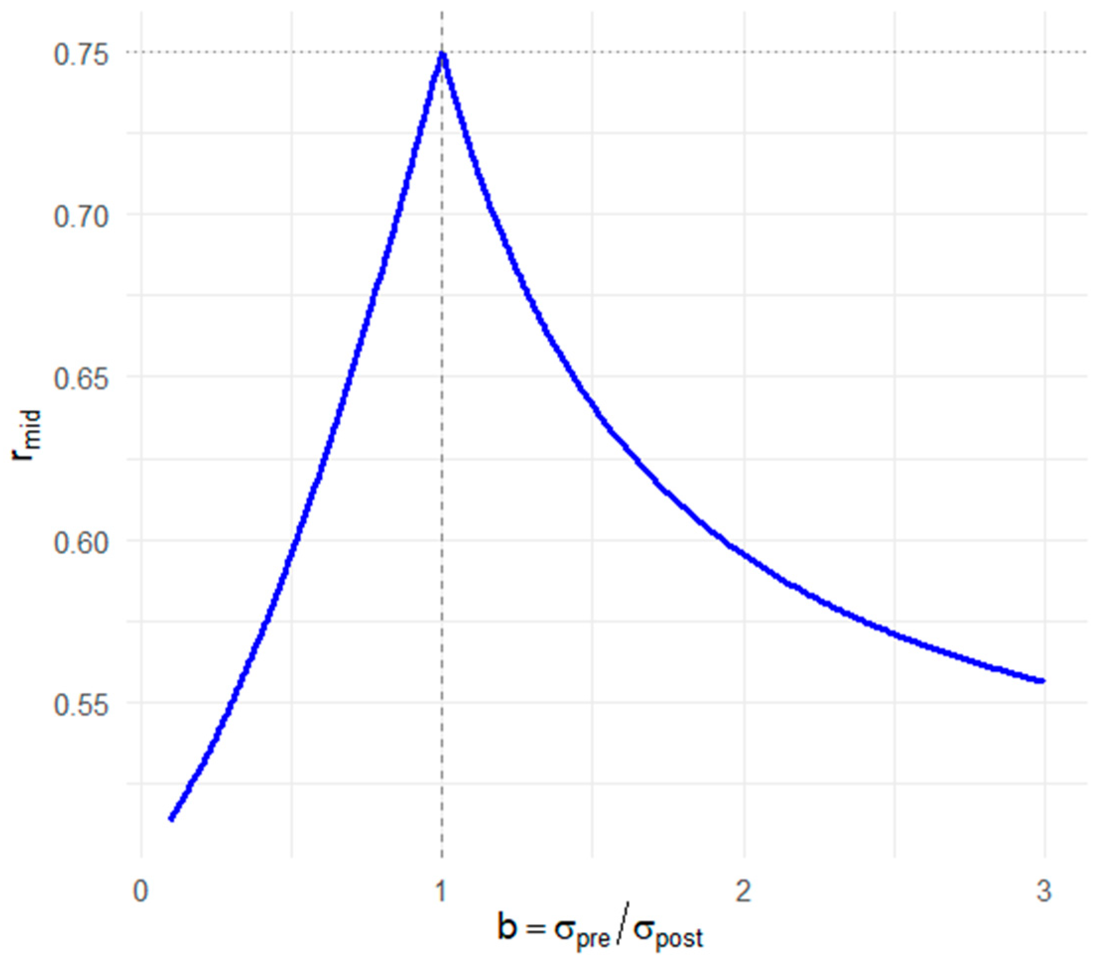
Solving for r, we get r = {b2 + 1 − {[|b − 1| + (b2 + 1)1/2]/2}2}/2b. The function r(b) is non-monotonic, with a peak at b = 1, where r = 0.75 (Figure 5).
Moreover, solving r = {b2 + 1 − {[|b − 1| + (b2 + 1)1/2]/2}2}/2b for b > 0, the empirically used r = 0.7 corresponds to b values of ~0.85 and ~1.17.

4. Discussion

This study provides a detailed and mathematically sound approach for the heuristic approximation of the correlation coefficient r between pre/post-values of continuous numerical variables in meta-analyses, particularly when r is absent or cannot be computed from the provided data. Moreover, our analysis shows how variation in assumed r influences derived metrics like σD, and we suggest that such assumptions be treated transparently and tested via sensitivity analysis when raw data are not available.
The proposed value of r = 0.75 is justified as it represents the midpoint between the minimum and the maximum variance of the pre/post-difference under the assumption of equal variances. The latter theoretical approach yields to symmetry in the Taylor approximation and could be reasonable in the absence of access to raw data. In this setting, any other arbitrarily chosen value, including the empirically used value of r = 0.7—though not strictly problematic—deviates from the described “mid-point” variance approach. Moreover, we have shown that the empirically used r = 0.7 corresponds to σpre/σpost = b values of ~0.85 and ~1.17 under the “midpoint hypothesis”. As such, r = 0.7 predisposes per se an asymmetry in pre/post-variances. Whether this might effectively buffer cluster-induced heterogeneity in variance structures remains to be investigated.
The initial assumption of r = 0.5 as the mean of the correlation distribution between pre/post-measurements in paired data is not derived from a formal mathematical theorem but rather reflects a long-standing empirical convention adopted across various applied disciplines. This assumption has been pragmatically used in statistical software (e.g., UNISTAT version 10), methodological guides (e.g., the Campbell Collaboration’s effect size calculator), and in the meta-analytic literature, where it often appears alongside sensitivity analyses exploring values such as 0.3, 0.5, and 0.7 [1,9].
Rosenthal proposed that, under the prerequisite of statistical significance, a value of 0.7 can be arbitrarily attributed to r, if it is unknown [8]. This approach has since been followed by various authors in the field of social research [4,5,7]. However, its use has rapidly extended to a wide range of fields, including biosciences [2,3,6,11,12,13]. As we have demonstrated, this approach does not equally counterbalance the under- and over-estimation of correlation-attributable variance when normality is met and equal pre/post-variance can be assumed. In contrast, implementing a value of r = 0.75 can accurately balance the variance deficit due to the correlation of paired data. Of note, we have demonstrated that all the above-mentioned values of r (either r = 0.5, r = 0.707, or r = 0.75) can tolerate a considerable amount of σr.
Whatever the assumption for r might be, the goal is to provide a reasonable estimate of the within-subject correlation, where a moderate effect is anticipated but not precisely known. Despite this assumption lacking a universal theoretical foundation, one may be tempted to justify it heuristically by noting that the correlation coefficient r takes values from the bounded interval [0, 1] (in pre/post-designs where positive correlation is expected) and that 0.5 might represent a midpoint or central tendency of plausible values in empirical settings. However, this is not a consequence of the CLT. While the CLT ensures that the sampling distribution of an estimated correlation becomes approximately normal with increasing sample size, it centers on the true population value of r—which remains unknown in many studies. Similarly, the Law of Large Numbers ensures that the mean of observed sample correlations across studies will converge on the true population mean, but again, this does not specify what that mean should be.
Beyond the need for approximation, an aspect that has been somewhat overlooked by many researchers is when μpre and μpost (pre- and post-means), σpre and σpost (pre- and post-standard deviations), n (sample size), and the p-value of the pre/post-difference are all known or can be directly computed by available data. In these cases, the true value of r can be computed, and therefore there is no need for an indirect approximation. In detail, (i) knowing the p-value, the t-value can be determined using inverse t-distribution; (ii) knowing the t-value, the Cohen’s d can be computed using the formula d = t/n1/2; (iii) the Cohen’s d can be converted to the correlation coefficient r via the formula r = d/(d2 + 4)1/2; and (iv) σD can be directly obtained as (σpre2 + σpost2 − 2preσpost)1/2. Solving for r from the latter, the well-established formula r = (σpre2 + σpost2σD2)/2σpreσpost, proposed by the Cochrane Collaboration, can be obtained [14].
While many prior approaches have relied on fixed assumptions of r, the present analysis introduces a probabilistic framework, modeling r as a normally distributed variable around the theoretical “true” mean. This strategy explicitly incorporates uncertainty and allows for plausible between-study variation in r, thereby improving the realism and robustness if the standard deviation estimates. However, this approach does not fully address potential cluster effects, which account for the systematic variation in correlation structure across studies due to shared methodological, contextual, or population-level factors [15,16]. The assumed normal distribution of r is independent across simulations and does not capture hierarchical relationships or structural dependencies due to, e.g., the same researchers. As such, the model may still underestimate total heterogeneity in the presence of latent clustering.
The primary limitation of this study is that the data used is simulated rather than real. Ideally, future research should explore how different assumptions about the correlation coefficient r—including both the empirically adopted value of r = 0.7 and the theoretically motivated r = 0.75—approximate results from real datasets, particularly under the assumption that pre- and post-intervention variances are equal. Additionally, this line of investigation should be extended to scenarios where pre- and post-variances are unequal. In such cases, it may be possible to identify a best-fitting value of r that depends on the ratio of pre- to post-variance b. The more extensive and diverse the datasets are, especially if they span a wide range of biomedical fields, the greater the potential validity and generalizability of the findings are anticipated to be.
Apart from r approximation, another valid approach is the implementation of a sensitivity analysis for different values of r. This method has been applied experimentally for r ∈ ℝ ∩ [0.5, 0.7] when pseudo-individual participant data is used to synthesize clinical study evidence [17]. A similar approach has been adopted in clinical meta-analyses by other researchers for a wide range of r values [18]. Additionally, the use of r derived from the raw data of even one study might further support the quality of the evidence [18]. In these cases, the correlation coefficient r can be further approximated as the mean of a distribution estimated via the maximum likelihood approach, assuming normality and a known variance. If the variance is unknown and cannot be approximated, at least three studies directly reporting r are required to estimate both the mean and the variance.

5. Conclusions

In conclusion, when r cannot be directly computed, it can be approximated; this study supports the use of r = 0.75, which represents half of the maximum variance that can be attributed to the correlation between paired data in the case of normality and equal variance. As such, we recommend using r = 0.75 as a default in the absence of raw data, paired with sensitivity analyses.

Funding

This research received no external funding.

Institutional Review Board Statement

Not applicable.

Informed Consent Statement

Not applicable.

Data Availability Statement

All data created are available upon reasonable request.

Acknowledgments

The author acknowledges that this article was partially generated by ChatGPT (powered by OpenAI’s language model, GPT-4; http://openai.com (accessed on 19 June 2025)). The editing was performed by the human author. In detail, ChatGPT was implemented to generate the R codes used for all Figures and to visualize them in the case of Figure 2 and Figure 4.

Conflicts of Interest

The author declares no conflicts of interest.

Appendix A

R code for Monte Carlo simulation of σD

# Load required libraries
library(ggplot2)
library(dplyr)

# Define parameters
mean_r_values <- c(0.5, 0.6, 0.707, 0.75, 0.8)
sigma_r_values <- c(0.05, 0.10, 0.15)
n <- 500000

# Fisher z-transform and inverse
fisher_z <- function(r) 0.5 * log((1 + r) / (1 − r))
inv_fisher_z <- function(z) tanh(z)

# Function to compute σD
compute_sigma_D <- function(r) sqrt(2 * (1 − r))

# Initialize empty data frame
results <- data.frame()

# Simulation loop
set.seed(123)
for (r_mean in mean_r_values) {
  z_mean <- fisher_z(r_mean)
  for (sigma_r in sigma_r_values) {
    z_samples <- rnorm(n, mean = z_mean, sd = sigma_r)
    r_samples <- inv_fisher_z(z_samples)
    sigma_D <- compute_sigma_D(r_samples)
    df <- data.frame(
      sigma_r = as.factor(sigma_r),
      sigma_D = sigma_D,
      Group = paste0(“r = ”, r_mean)
    )
    results <- bind_rows(results, df)
  }
}

# Boxplot visualization
ggplot(results, aes(x = sigma_r, y = sigma_D, fill = Group)) +
  geom_boxplot(outlier.size = 0.5, coef = 2) +
  labs(
    title = expression(“Monte Carlo Simulation of” ~ sigma[D]),
    subtitle = “500,000 samples per group”,
    x = expression(sigma[r]),
    y = expression(sigma[D]),
    fill = “Mean r”
  ) +
  theme_minimal(base_size = 14) +
  theme(legend.position = “right”)

References

  1. UNISTAT Statistics Software. 6.8.3. Summary of Effect Sizes. Available online: https://www.unistat.com/guide/meta-analysis-summary-of-effect-sizes/?utm_source=chatgpt.com (accessed on 17 June 2025).
  2. Socha, M.; Pietrzak, A.; Grywalska, E.; Pietrzak, D.; Matosiuk, D.; Kiciński, P.; Rolinski, J. The effect of statins on psoriasis severity: A meta-analysis of randomized clinical trials. Arch. Med. Sci. 2019, 16, 1–7. [Google Scholar] [CrossRef] [PubMed]
  3. Papadopoulos, V.P.; Apergis, N.; Filippou, D.K. Nocturia in CPAP-treated obstructive sleep apnea patients: A systematic review and meta-analysis. SN Comprehens. Clin. Med. 2020, 2, 2799–2807. [Google Scholar] [CrossRef]
  4. Manser, P.; Herold, F.; de Bruin, E.D. Components of effective exergame-based training to improve cognitive functioning in middle-aged to older adults—A systematic review and meta-analysis. Ageing Res. Rev. 2024, 99, 102385. [Google Scholar] [CrossRef] [PubMed]
  5. Chin, P.; Gorman, F.; Beck, F.; Russell, B.R.; Stephan, K.E.; Harrison, O.K. A systematic review of brief respiratory, embodiment, cognitive, and mindfulness interventions to reduce state anxiety. Front. Psychol. 2024, 15, 1412928. [Google Scholar] [CrossRef] [PubMed]
  6. Obomsawin, A.; Pejic, S.R.; Koziol, C. Effects of racial discrimination tasks on salivary cortisol reactivity among racially minoritized groups: A meta-analysis. Horm. Behav. 2025, 173, 105775. [Google Scholar] [CrossRef] [PubMed]
  7. McGirr, A.; Berlim, M.T.; Bond, D.J.; Neufeld, N.H.; Chan, P.Y.; Yatham, L.N.; Lam, R.W. A systematic review and meta-analysis of randomized controlled trials of adjunctive ketamine in electroconvulsive therapy: Efficacy and tolerability. J. Psychiatr. Res. 2015, 62, 23–30. [Google Scholar] [CrossRef] [PubMed]
  8. Rosenthal, R. Meta-Analytic Procedures for Social Research; Applied Social Research Methods Series 6; Sage Publications: Newbury Park, CA, USA, 1991. [Google Scholar]
  9. Campbell Collaboration and Effect-Size Calculators. Available online: https://www.campbellcollaboration.org/calculator/equations?utm_source=chatgpt.com (accessed on 17 June 2025).
  10. Van der Vaart, A.W. Asymptotic Statistics; Cambridge University Press: Cambridge, UK, 1998. [Google Scholar]
  11. Yagiz, G.; Akaras, E.; Kubis, H.-P.; Owen, J.A. The Effects of Resistance Training on Architecture and Volume of the Upper Extremity Muscles: A Systematic Review of Randomised Controlled Trials and Meta-Analyses. Appl. Sci. 2022, 12, 1593. [Google Scholar] [CrossRef]
  12. Meléndez-Oliva, E.; Martínez-Pozas, O.; Cuenca-Zaldívar, J.N.; Villafañe, J.H.; Jiménez-Ortega, L.; Sánchez-Romero, E.A. Efficacy of Pulmonary Rehabilitation in Post-COVID-19: A Systematic Review and Meta-Analysis. Biomedicines 2023, 11, 2213. [Google Scholar] [CrossRef] [PubMed]
  13. Herrero, P.; Val, P.; Lapuente-Hernández, D.; Cuenca-Zaldívar, J.N.; Calvo, S.; Gómez-Trullén, E.M. Effects of Lifestyle Interventions on the Improvement of Chronic Non-Specific Low Back Pain: A Systematic Review and Network Meta-Analysis. Healthcare 2024, 12, 505. [Google Scholar] [CrossRef] [PubMed]
  14. Higgins, J.P.T.; Thomas, J.; Chandler, J.; Cumpston, M.; Li, T.; Page, M.J.; Welch, V.A. (Eds.) Cochrane Handbook for Systematic Reviews of Interventions, version 6.5; updated August 2024; Cochrane: London, UK, 2024. Available online: www.cochrane.org/authors/handbooks-and-manuals/handbook/current/chapter-06#section-6-5-2-8 (accessed on 2 August 2025).
  15. Olkin, I.; Pratt, J.W. Unbiased estimation of certain correlation coefficients. Ann. Math. Stat. 1958, 29, 201–211. [Google Scholar] [CrossRef]
  16. Zimmerman, D.W.; Williams, R.H.; Zumbo, B.D. Effect of nonindependence of sample observations on some parametric and nonparamentric statistical tests. Commun. Stat.—Simul. Comput. 1993, 22, 779–789. [Google Scholar] [CrossRef]
  17. Papadimitropoulou, K.; Stijnen, T.; Riley, R.D.; Dekkers, O.M.; le Cessie, S. Meta-analysis of continuous outcomes: Using pseudo IPD created from aggregate data to adjust for baseline imbalance and assess treatment-by-baseline modification. Res. Synth. Methods 2020, 11, 780–794. [Google Scholar] [CrossRef] [PubMed]
  18. Papadopoulos, V.P.; Mimidis, K. Corrected QT interval in cirrhosis: A systematic review and meta-analysis. World J. Hepatol. 2023, 27, 1060–1083. [Google Scholar] [CrossRef] [PubMed]
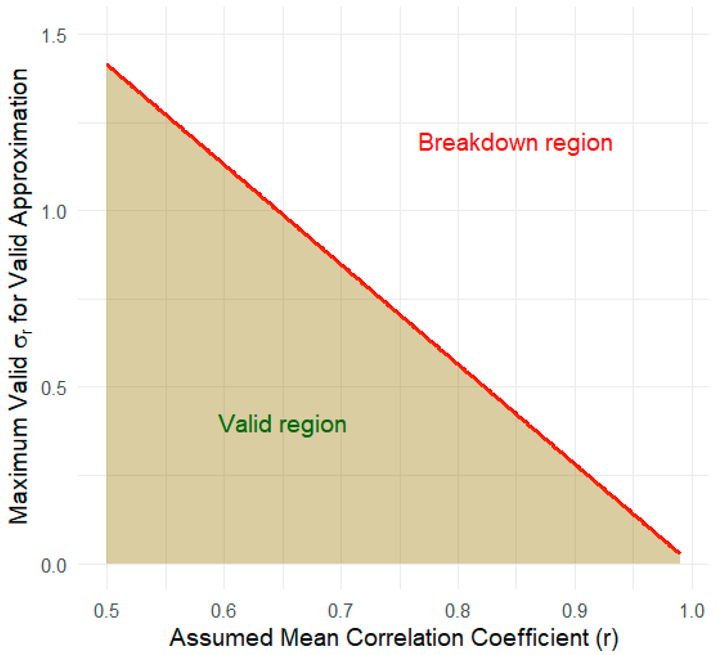
Figure 1. Graphic representation of σr(crit) depicting the validity of Taylor approximation for ℮|σD|; the green-shaded region indicates safe (valid) combinations of r and σr, where the Taylor expansion yields positive, interpretable results.
Stats 08 00072 g001
Figure 2. Graphic representation of the function σD = [2σ2(1 − r)]1/2 for r = 0.707.
Stats 08 00072 g002
Figure 3. A box-and-whisker plot depicting the results of the 500,000 simulations per case for the expected σD under five scenarios for r (r = 0.5, r = 0.6, r = 0.707, r = 0.75, and r = 0.8), each examined for three levels of σr (0.05, 0.1, and 0.15).
Stats 08 00072 g003
Figure 4. Limit behavior of ℮|σD| versus σr2 for the five scenarios (r = 0.5, r = 0.6, r = 0.707, r = 0.75, and r = 0.8) of σD.
Stats 08 00072 g004
Figure 5. Plot showing the proposed r under “midpoint” hypothesis.
Stats 08 00072 g005
Disclaimer/Publisher’s Note: The statements, opinions and data contained in all publications are solely those of the individual author(s) and contributor(s) and not of MDPI and/or the editor(s). MDPI and/or the editor(s) disclaim responsibility for any injury to people or property resulting from any ideas, methods, instructions or products referred to in the content.