Article

Unraveling Similarities and Differences Between Non-Negative Garrote and Adaptive Lasso: A Simulation Study in Low- and High-Dimensional Data

Institute of Medical Biometry and Statistics, Faculty of Medicine and Medical Center, University of Freiburg, Stefan-Meier-Street 26, 79104 Freiburg, Germany
*
Author to whom correspondence should be addressed.
Stats 2025, 8(3), 70; https://doi.org/10.3390/stats8030070
Submission received: 8 July 2025 / Revised: 31 July 2025 / Accepted: 3 August 2025 / Published: 6 August 2025
(This article belongs to the Section Statistical Methods)

Abstract

Penalized regression methods are widely used for variable selection. Non-negative garrote (NNG) was one of the earliest methods to combine variable selection with shrinkage of regression coefficients, followed by lasso. About a decade after the introduction of lasso, adaptive lasso (ALASSO) was proposed to address lasso’s limitations. ALASSO has two tuning parameters ( λ and γ ), and its penalty resembles that of NNG when γ = 1 , though NNG imposes additional constraints. Given ALASSO’s greater flexibility, which may increase instability, this study investigates whether NNG provides any practical benefit or can be replaced by ALASSO. We conducted simulations in both low- and high-dimensional settings to compare selected variables, coefficient estimates, and prediction accuracy. Ordinary least squares and ridge estimates were used as initial estimates. NNG and ALASSO ( γ = 1 ) showed similar performance in low-dimensional settings with low correlation, large samples, and moderate to high R 2 . However, under high correlation, small samples, and low R 2 , their selected variables and estimates differed, though prediction accuracy remained comparable. When γ 1 , the differences between NNG and ALASSO became more pronounced, with ALASSO generally performing better. Assuming linear relationships between predictors and the outcome, the results suggest that NNG may offer no practical advantage over ALASSO. The γ parameter in ALASSO allows for adaptability to model complexity, making ALASSO a more flexible and practical alternative to NNG.

1. Introduction

Penalized regression methods are widely used in statistical modeling, with applications in both low- and high-dimensional settings where many candidate predictors are available but only a small subset influences the outcome [1,2,3,4,5]. Accurately identifying these relevant predictors improves both the predictive performance and interpretability of fitted models [1,4,6], which are key goals in many fields, including economics, finance, engineering, and health sciences [3].
Non-negative garrote (NNG) [7] and adaptive lasso (ALASSO) [6] are examples of penalized regression methods that perform variable selection and shrinkage of regression coefficients simultaneously. A common view in the literature is that NNG is simply a special case of ALASSO. This is based on earlier theoretical work [6], which showed that the NNG can be expressed as the ALASSO ( γ = 1 ) with an additional sign constraint. However, this constraint is often overlooked, leading to the mistaken belief that the two methods are interchangeable. As ALASSO continues to gain popularity due to its theoretical properties, particularly its ability to yield sparser models [8], it is important to assess how it compares to NNG under varying conditions and determine whether it can serve as a practical substitute. Therefore, a systematic performance comparison is necessary in order to guide method selection in applied research.
The NNG combines the simplicity of subset selection with the predictive accuracy and computational efficiency of ridge regression, resulting in models that are simpler than those produced by ridge regression and more accurate than those selected based on subset [7]. Although originally proposed for normal-error regression models, it has since been extended to generalized linear models [9] and additive models [10]. Recently, it has been employed for variable selection in complex settings involving zero-inflated and highly correlated predictors [11].
The original NNG relies on both the sign and magnitude of the ordinary least squares (OLS) estimates from the full model as initial estimates in low-dimensional settings. This can be problematic when covariates are highly correlated or when the sample size is small, as it leads to high variance and unreliable OLS estimates. Moreover, OLS estimates are not available in high-dimensional settings, which explains why NNG has not been widely applied in such contexts [12]. To address these limitations, alternative initial estimates such as those derived from ridge and lasso regression models have been proposed, making it possible to use NNG to analyze both high-correlation and high-dimensional data [11,13,14,15]. These initial estimates allow NNG to shrink coefficients differentially by assigning larger and smaller penalties to coefficients with smaller and larger initial estimates, respectively. This helps to avoid overshrinkage of large effects that require minimal shrinkage [13].
Recognizing the limitations of the NNG’s reliance on initial estimates, Tibshirani [16,17] proposed the lasso method, which uses an 1 penalty term and can be applied to both low- and high-dimensional data. While lasso has been successful in many applications, it also has a number of weaknesses [18]. First, it is not consistent for variable selection [6], which means that even as the sample size increases, the probability of correctly selecting only the true set of relevant (signal) variables does not approach one. In order for consistency to hold, the design matrix X must satisfy a strong condition known as the irrepresentable condition [6,19,20]. This condition requires that the signal variables are not strongly correlated with each other and are only weakly correlated with the noise variables [19,21]. Otherwise, the lasso may not be able to distinguish between signal and noise variables regardless of the amount of data or regularization [19,22,23,24]. Verifying this condition in real data is challenging because the true underlying model is unknown [19]. Second, even when lasso achieves consistency in variable selection, it is not efficient in estimating the coefficients of nonzero components because the tuning parameter that ensures consistency tends to overshrink these coefficients, leading to excessive bias [8]. Third, lasso’s penalty uniformly shrinks both small and large nonzero coefficients, resulting in asymptotically biased estimates for large coefficients [6]. To address these weaknesses, ALASSO was proposed [6].
ALASSO relaxes the stringent conditions that lasso imposes on the design matrix to achieve consistency in variable selection by using a weighted 1 penalty with weights derived from initial estimates [6,20]. These adaptive weights are crucial for applying different levels of penalization to the regression coefficients, which improves variable selection accuracy and reduces the estimation bias commonly associated with lasso, particularly for large coefficients [6]. For a fixed number of covariates, ALASSO has been shown to possess the oracle property, whereas lasso does not [6,25]. The oracle property states that as the sample size increases, the probability of the selected model including exactly the true set of signal variables approaches one. In addition, the corresponding parameter estimates are asymptotically normal, with the same mean and covariance as those obtained under maximum likelihood estimation if the true submodel were known in advance [6,25]. In other words, the oracle property guarantees consistency of variable selection and ensures that the estimates for the selected model are asymptotically unbiased [21].
ALASSO and NNG share several similarities. Both rely on initial estimates, and as such face similar challenges associated with those estimates. They also exhibit similar shrinkage behavior, shrinking small and large coefficients differently depending on the magnitude of the initial estimates. However, they differ in three main aspects. First, the NNG has a single tuning parameter ( λ ), whereas ALASSO has two tuning parameters ( λ and γ ), making ALASSO more computationally intensive when both parameters are tuned simultaneously. Moreover, having more tuning parameters can increase instability, especially in small samples [1,26,27]. To mitigate this, some researchers fix γ at a certain positive value and focus on tuning λ [20]. Second, NNG depends on both the sign and magnitude of the initial estimates, whereas ALASSO relies only on their magnitude [6,16]. Specifically, NNG requires that the signs of its nonzero coefficients match those of the initial estimates, while ALASSO permits sign changes [6]. As a result, the signs of the initial estimates are critical for model selection in NNG, as an incorrect sign can lead to the exclusion of the corresponding variable.
In summary, ALASSO is more flexible than NNG due to its γ parameter, which can be advantageous in complex situations as it allows for heavy shrinkage when appropriate and reduces it when less necessary. However, the need to tune two parameters can be problematic, particularly in small samples, where the parameters may exhibit high variability and increase the variance of the prediction error [28].
As previously mentioned, NNG can theoretically be regarded as a special case of ALASSO with γ = 1 and additional sign constraints [6]. Despite this conceptual connection, few comparative studies have evaluated the practical similarities and differences between the two methods across a range of conditions. To the best of our knowledge, no simulation study has systematically compared NNG and ALASSO in both low- and high-dimensional settings, nor explored how the tuning parameter γ affects ALASSO’s performance relative to NNG. This study addresses this gap through simulation studies under normal-error regression models in both low- and high-dimensional settings. The specific objectives are as follows: first, to identify scenarios in which NNG and ALASSO ( γ = 1 ) yield similar or different results, focusing on selected variables, coefficient estimates, and prediction accuracy; second, to assess the impact of incorrect signs in the initial estimates on model selection in both methods; and finally, to evaluate the effect of varying the ALASSO tuning parameter γ (with values 0.5, 1, and 2) on model complexity and predictive performance. For both approaches, we use OLS and ridge estimates as initial estimates, with the ridge tuning parameter selected using 10-fold cross-validation (CV). OLS is used only in low-dimensional settings, whereas ridge estimates are used in both low- and high-dimensional settings.
Throughout, we standardize each covariate in the training data to have a mean of zero and unit variance. Additionally, we center the response variable by its mean to omit the intercept from the model. All variables in the new dataset are standardized using the statistics derived from the training data.
Section 2 describes the simulation design, which is organized according to the ADEMP structure [29]. This framework entails defining the aims (A), data-generating mechanisms (D), estimands (or targets of analysis) (E), methods (M), and performance measures (P), which are covered in the following subsections: Section 2.1 provides a brief overview of the overall simulation design; Section 2.2 provides the data-generating mechanisms; and Section 2.3 discusses the performance measures. In addition, Section 2.4 provides a detailed explanation of the methods, while Section 2.5 introduces the notation used throughout the paper. The simulation results are reported in Section 3.1 and Section 3.2, which summarize the findings for the low- and high-dimensional settings, respectively. Section 3.3 presents the results of a real data example. Finally, Section 4 discusses the findings, Section 5 summarizes the main conclusions, and Section 6 outlines directions for future research.

2. Materials and Methods

2.1. Simulation Design

We used a subset of the simulation parameters from a previously published protocol for low-dimensional settings [14] (see Table S1 in File S1) and introduced additional parameters to assess the performance of the approaches in high-dimensional settings (Section 2.2). Table 1 summarizes our simulation study using the ADEMP structure, clearly stating the aims and targets of the analysis. We provide detailed discussions on the data-generating mechanisms in Section 2.2, performance measures in Section 2.3, and methods in Section 2.4.

2.2. Data-Generating Mechanisms

We generated 10,000 training datasets per scenario for low-dimensional settings to ensure that the Monte Carlo standard error (MCSE) of the model error (ME) was smaller than 0.005. This level of precision allows for models that consistently outperform others by a large margin to be reasonably regarded as superior, as is common practice in simulation studies. For high-dimensional settings, we generated 1000 datasets due to computational complexity. Each training dataset consisted of a continuous response variable y and 15 continuous covariates (7 signal and 8 noise) for low-dimensional data and 1000 covariates (7 signal and 993 noise) for high-dimensional data. The covariate matrix X was sampled from a multivariate normal distribution with a mean vector of zero and a covariance matrix Σ , with Σ i j as the correlation coefficient between covariates x i and x j . In low-dimensional settings, we considered both low- and high-correlation settings, whereas in high-dimensional settings only low correlation was considered in order to avoid additional challenges posed by high correlation (Table 1). Each covariate was standardized to have a mean of zero and unit variance before generating y.
For y, we used the formula y = X β + ϵ , where β is a vector of true regression coefficients, with some elements set to zero to represent noise variables (see Table 1). The error term ϵ i was sampled from a normal distribution with a mean of zero and variance σ 2 . The residual variance σ 2 was determined from R 2 using the following expression [23]:
R 2 = var ( X T β ) σ 2 + var ( X T β ) = β T Σ β σ 2 + β T Σ β
which leads to
σ 2 = β T Σ β 1 R 2 R 2 .
In the low-dimensional setting, we considered 12 different scenarios by varying three R 2 values (0.20, 0.50, and 0.80), two sample sizes (n = 100 and 400), and two correlation structures (C2: low correlation and C4: high correlation). This allowed us to evaluate the performance of methods under (i) low, moderate, and high R 2 ; (ii) small and large sample sizes; and (iii) low and high correlations. In high-dimensional settings, we considered six scenarios by varying two sample sizes (n = 100 and 400) and three R 2 values (0.20, 0.50 and 0.80). In real data, sample sizes can be less than 100; however, such cases were not included in this study.
To test how well the models performed on the new dataset, we generated an independent test dataset with a large sample size of 100,000 using the same design as the training data. A large test dataset provides more accurate and reliable prediction results due to reduced variance in performance measures [31]. To reduce the influence of extreme values or outliers in the covariates, each covariate x j was truncated after the response variable y was generated. This approach ensures that the truncation affects only the model fitting process and not the data-generating mechanism. Truncating extreme values without deleting observations is generally considered acceptable, particularly in simulation studies involving many repetitions. Specifically, within each simulated dataset, values of x j below the empirical first percentile were set equal to the first percentile, with values above the 99th percentile set equal to the 99th percentile.

2.3. Performance Measures

We grouped the performance measures into three categories: variable selection (Section 2.3.1), regression estimates (Section 2.3.2), and prediction accuracy (Section 2.3.3).

2.3.1. Variable Selection

In penalized regression methods that perform variable selection, coefficients are either nonzero (selected variables) or zero (excluded variables). These coefficients can be represented as 1 for nonzero and 0 for zero, forming a binary vector. When two methods select the same variables, their binary vectors are identical. To quantify the similarity between selection results, we used the simple matching coefficient (SMC). In addition, model performance was evaluated using the false positive rate (FPR), false negative rate (FNR), and Matthews correlation coefficient (MCC).
Simple Matching Coefficient
To determine whether NNG and ALASSO selected the same variables, we compared the similarity between their binary selection vectors using SMC, a widely used similarity measure [32]. For illustration, consider five covariates, with NNG producing the binary vector [ 1 , 0 , 1 , 1 , 0 ] and ALASSO producing [ 1 , 1 , 0 , 1 , 0 ] . These vectors can be summarized in a 2 × 2 contingency table (Table 2). The sum of the diagonal entries ( a + d ) represents the number of covariates that both methods either selected or excluded (i.e., matching outcomes), while the off-diagonal entries ( b + c ) represent the number of mismatches.
The SMC is calculated as follows:
SMC = a + d a + b + c + d = a + d p ,
where p is the total number of variables; in our example, p = 5 . An SMC of 0 indicates that the two methods selected completely different variables ( a = d = 0 ), whereas an SMC of 1 indicates that the two methods selected the same variables ( b = c = 0 ). In our hypothetical example, the SMC is 0.6, indicating a moderate level of similarity between the two approaches, with 60% (both 1s and 0s) of the variables matching.
False Positive Rates and False Negative Rates
The SMC provides a single numerical value that quantifies the similarity between two approaches based on their variable selection. However, it does not indicate how well each method distinguishes signal from noise variables, given that the true underlying model is known in the simulation setup. This distinction is crucial for evaluating model performance, especially when models are intended for descriptive purposes.
To address this limitation, we used the additional measures of FPR and FNR. For each replication of a scenario, we computed these metrics for each variable selection approach. The FPR ranges from 0 to 1; values close to 1 indicate that many noise variables are incorrectly selected, which can lead to overfitting, whereas a value of 0 indicates that no noise variables are selected. The FNR also ranges from 0 to 1; values near 1 indicating that many signal variables are eliminated, which can lead to underfitting, whereas a value of 0 indicates that no signal variables are eliminated.
We computed the overall FPR and FNR for each approach in a given scenario by averaging the respective values across all replications, then used them to compare the approaches. An ideal variable selection method minimizes both FPR and FNR.
Matthews Correlation Coefficient
The MCC [33] and the F1 score [34] are two widely used metrics for evaluating the performance of binary classifiers. In imbalanced classification problems, where one class has substantially more observations than the other, the F1 score can be misleading because it does not account for true negatives (TNs) [35,36]. Moreover, the F1 score is sensitive to class labeling; its value may change if the positive and negative classes are swapped, whereas the MCC is invariant to such changes [36]. For this reason, MCC is often preferred, as it considers all four elements of the 2 × 2 contingency table, namely, true negatives (TNs), true positives (TPs), false positives (FPs), and false negatives (FNs), providing a more robust and reliable evaluation [36].
In this study, we used the MCC to assess the performance of NNG and ALASSO, particularly because the number of signal variables (7) differed from the number of noise variables (8 in the low-dimensional setting and 993 in the high-dimensional setting). The MCC is calculated as shown below.
MCC = ( T P × T N ) ( F P × F N ) ( T P + F P ) ( T P + F N ) ( T N + F P ) ( T N + F N )
The MCC yields a high score only when the variable selection method correctly identifies most signal and noise variables, resulting in a large number of TPs and TNs [36]. The MCC ranges from 1 to + 1 , with 1 indicating perfect misclassification of variables as signal or noise, + 1 indicating perfect classification, and 0 reflecting performance no better than random chance [36].

2.3.2. Regression Estimates

Manhattan Distance
The regression coefficients from NNG and ALASSO are continuous vectors on the same scale, as the covariates were standardized. To quantify differences between such vectors, the Euclidean and Manhattan distances are commonly used. In this study, we used the Manhattan distance (MD) instead of the Euclidean distance to prevent large differences in individual coefficients from disproportionately affecting the overall measure. While such differences should contribute to the distance, they should not dominate it, as can occur under the Euclidean distance, which squares the differences [37].
Let A = ( a 1 , , a k ) and B = ( b 1 , , b k ) be two vectors of length k. The MD between A and B is defined as
MD ( A , B ) = i = 1 k | a i b i | ,
which is the sum of the absolute differences between corresponding elements of the two vectors. An MD of 0 indicates that the regression coefficients from NNG and ALASSO are identical, while larger values indicate substantial differences. To simplify interpretation and avoid negligible differences that may result from numerical precision, all MD values less than 0.001 were set to zero. This allowed us to focus on meaningful differences.

2.3.3. Prediction Accuracy

Relative Test Error
The relative test error (RTE) quantifies the expected test error relative to the Bayes error rate [23]. The RTE is a standardized form of the mean squared prediction error [38], and is defined as follows:
R T E β ^ = E y 0 X 0 T β ^ 2 σ 2 = β ^ β T Σ β ^ β + σ 2 σ 2 = M E + σ 2 σ 2 ,
where X 0 denotes a random matrix of test covariates, y 0 is a random vector of test response variable, β is a vector of true coefficients, and β ^ is a vector of estimated coefficients from a regression method. The term β ^ β T Σ β ^ β represent the model error (ME). The numerator of the RTE is the mean squared prediction error, which can be decomposed into two components: the ME and the noise variance σ 2 . The first component is the prediction error due to lack of fit to the underlying model, while the second captures irreducible error due to noise [7]. The denominator rescales the expression by σ 2 to aid interpretation [15]. A null model (model without predictors) has an RTE score of β T Σ β + σ 2 / σ 2 = SNR + 1 , whereas a perfect model β ^ = β has a score of 1, since ME = 0. A good prediction model should have an RTE close to 1 [23,38].

2.4. Methods

ALASSO (Section 2.4.1) and NNG (Section 2.4.2) have been extensively studied in the literature [6,13,14,15]. Below, we provide a brief overview of their fundamental concepts to help in understanding their similarities and differences.

2.4.1. Adaptive Lasso

For the classical linear regression model with standardized covariates and a centered response variable, the ALASSO estimates are obtained by minimizing the following objective function with respect to β ALASSO R p :
1 2 n i = 1 n y i j = 1 p x i j β j ALASSO 2 + λ j = 1 p | β j ALASSO | | β ^ j init | γ , subject to λ 0 and γ > 0
where β j ALASSO denotes the ALASSO coefficient for the j-th predictor, β ^ j init is an initial estimate obtained from OLS or ridge regression, and λ and γ are tuning parameters. The adaptive weights, defined as w j * = | β ^ j init | γ , depend on the initial estimates and the value of γ . When γ = 0 , all weights are equal to one, reducing ALASSO to standard lasso.
An equivalent method for obtaining ALASSO estimates using the standard lasso algorithm was proposed in [6]. Specifically, for a given γ value, the covariates are rescaled as x i j * = x i j | β ^ j init | γ , where x i j is the j-th covariate value for observation i. The ALASSO shrinkage factors c ^ * ( λ , γ ) = ( c ^ 1 * ( λ , γ ) , , c ^ p * ( λ , γ ) ) are obtained by minimizing the following objective function with respect to c * R p :
1 2 n i = 1 n y i j = 1 p c j * x i j * 2 + λ j = 1 p | c j * | , subject to λ 0 .
This objective function is identical to that of the standard lasso method, and its solution c ^ * corresponds to the lasso estimates on the rescaled covariates. The final ALASSO estimates are then calculated as follows:
β ^ j ALASSO ( λ , γ ) = c ^ j * ( λ , γ ) | β ^ j init | γ
indicating that the ALASSO estimates depend on the initial estimates as well as on the tuning parameters λ and γ .
The shrinkage factor c ^ j * can be negative because the rescaling uses the absolute values of the initial estimates. In contrast, all shrinkage factors in NNG must be non-negative due to the non-negativity constraint imposed on its objective function (see Section 2.4.2).
ALASSO has two tuning parameters, λ and γ , which are typically selected via two-dimensional CV. In this study, we tuned only λ using one-dimensional 10-fold CV and selected the value that minimized the mean squared error (MSE). The parameter γ was fixed at 0.5, 1, and 2 to evaluate its impact on variable selection and prediction. Initial estimates were obtained from either OLS or ridge regression. For ridge regression, the tuning parameter was selected via 10-fold CV by minimizing the MSE.

2.4.2. Non-Negative Garrote

Given a set of initial estimates β ^ init , NNG rescales the covariates as x i j * * = x i j β ^ j init , which differs from ALASSO, where they are rescaled as x i j * = x i j | β ^ j init | γ for some γ > 0 . Unlike ALASSO, NNG does not have a γ parameter and can be interpreted as implicitly setting it to 1. For classical linear regression models with standardized covariates and a centered response variable, the NNG shrinkage factors c ^ * * ( λ ) = ( c ^ 1 * * ( λ ) , , c ^ p * * ( λ ) ) are obtained by minimizing the following objective function with respect to c * * R p :
1 2 n i = 1 n y i j = 1 p c j * * x i j * * 2 + λ j = 1 p c j * * , subject to c j * * 0 , λ 0 .
This objective function is equivalent to the standard lasso objective with an added non-negativity constraint on the coefficients, since the penalty term λ j = 1 p c j * * is equal to λ j = 1 p | c ^ j * * | under the constraint c j * * 0 . Consequently, optimization can be performed using the standard lasso algorithms by setting the lower bounds of the coefficients to zero in order to obtain the NNG shrinkage factors. In practice, this can be implemented using the glmnet package (version 4.1-9) [39] in R software (version 4.5.1) [40] by setting the lower.limits argument to zero, which enforces the non-negativity constraint during optimization.
After the shrinkage factors are obtained, the final NNG estimates are calculated as
β ^ j NNG ( λ ) = c ^ j * * ( λ ) β ^ j init ,
which are scaled versions of the initial estimates, with the amount of scaling depending on the tuning parameter λ . When λ = 0 , the penalty term has no effect and all shrinkage factors equal 1, reducing the NNG model to the initial model. In particular, if the initial estimates are taken to be the OLS estimates, then the NNG model reduces to the OLS solution. Conversely, when λ is sufficiently large, all shrinkage factors are equal to zero, reducing the NNG model to an intercept-only model.
Unlike ALASSO, the NNG shrinkage factors are constrained to be non-negative. To preserve the direction of the relationship between the outcome and covariates, the NNG retains the sign of the initial estimates for nonzero coefficients. This can be problematic if the initial estimates have incorrect signs, as the model retains these erroneous signs or incorrectly eliminates important variables. This is more likely to occur for variables with weak effects and unlikely for those with strong effects.
Given that c j * * = β j NNG / β ^ j init and | c ^ j * * | = c ^ j * * for c ^ j * * 0 , the NNG objective function (Equation (3)) can equivalently be reformulated as follows [6,16]:
1 2 n i = 1 n y i j = 1 p β j NNG x i j 2 + λ j = 1 p | β j NNG | | β ^ j init | , subject to β j NNG β ^ j init 0 , λ 0 .
This function is identical to the ALASSO ( γ = 1 ) objective function (Equation (1)) but with an additional constraint that β j NNG / β ^ j init 0 , which is equivalent to β j NNG β ^ j init 0 [6]. This constraint indicates that NNG and ALASSO ( γ = 1 ) may yield different solutions, as NNG can only assign a nonzero coefficient to a variable if the sign of the estimated coefficient matches that of the corresponding initial estimate.
The NNG weights are calculated as w j * * = | β ^ j init | 1 , which is identical to the weights for ALASSO ( γ = 1 ) (see Section 2.4.3 for further details). The OLS and ridge initial estimates used for ALASSO were also employed in NNG to facilitate comparisons between the two methods. One-dimensional 10-fold CV was used to select λ by minimizing the MSE.

2.4.3. Adaptive Lasso Versus Non-Negative Garrote Weights

As previously mentioned, both ALASSO and NNG construct weights using initial estimates. For a given covariate x j , the weight is defined in ALASSO as w ^ j * = | β ^ j init | γ and in NNG as w ^ j * * = | β ^ j init | 1 . These weights are identical when γ = 1 and differ when γ 1 . Because each x j is standardized, covariates with stronger effects tend to have larger standardized initial estimates, yielding smaller weights; in contrast, covariates with weaker effects have initial estimates closer to zero, leading to larger weights. This weighting scheme shrinks estimates for weaker effects more severely than those for stronger effects.
Consider a hypothetical vector of standardized initial estimates β ^ init = ( 0.01 , 0.05 , 1.5 , 4 ) , ordered from weakest to strongest effect. Table 3 presents the corresponding weights for NNG and ALASSO across different values of γ . For ALASSO, a smaller value of γ = 0.5 yielded a weight of 10 for a covariate with an initial estimate of 0.01, whereas a larger value of γ = 2 resulted in a weight of 10,000 for the same initial estimate. This illustrates that for a fixed λ , ALASSO with larger γ values imposes more severe shrinkage on smaller coefficients while applying minimal shrinkage to larger ones.
As expected, the weights for NNG and ALASSO ( γ = 1 ) were identical but smaller than those for ALASSO ( γ = 2 ) when the initial estimates were small. This implies that a larger tuning parameter is required for NNG or ALASSO ( γ = 1 ) to select the same model as ALASSO ( γ = 2 ), which may lead to more shrinkage of large effects (see Section 2.4.4 for an example).

2.4.4. Orthonormal Design

To gain insights into the shrinkage behavior of NNG and ALASSO, we consider an orthonormal design in which each covariate x j is independently drawn from a standard normal distribution, x j N ( 0 , 1 ) and all covariates are uncorrelated [16]. Under these conditions, the design matrix X satisfies X X / n = I p × p , that is, the p × p identity matrix [16,20]. In this setting, both NNG and ALASSO have closed-form solutions when using OLS initial estimates, respectively provided by
β ^ j NNG ( λ ) = 1 λ ( β ^ j * ) 2 + β ^ j * and β ^ j ALASSO ( λ , γ ) = sign ( β ^ j * ) | β ^ j * | λ | β ^ j * | γ + ,
where ( z ) + = max ( 0 , z ) denotes the positive part of z, β ^ j * is the OLS estimate for x j from the full model, and sign ( β ^ j * ) denotes the sign of the OLS estimate, where sign ( β ^ j * ) = 1 if β ^ j * < 0 and + 1 if β ^ j * > 0 , as all OLS estimates are nonzero [6,16]. These closed-form expressions show that NNG and ALASSO ( γ = 1 ) produce identical solutions under an orthonormal design [20]. However, in more general settings with correlated covariates, the solutions may differ [6].

A Toy Example Illustrating Orthonormal Design

In this example, we compare the shrinkage behavior of NNG and ALASSO with γ { 0.5 , 1 , 2 , 10 } in an orthonormal setting. We generated a dataset of size n = 10 , 000 using the linear model y = X β + ε , where the true coefficients were β = ( 0.05 , 0.10 , 0.20 , 0.30 , 0.40 , 0.90 , 1.20 , 1.50 , 2 , 4 ) and the error terms were independently drawn from N ( 0 , 1 ) . Each covariate x j was independently sampled from N ( 0 , 1 ) , and the covariates were uncorrelated. To facilitate comparison, we fixed λ = 0.1 across all methods.
Table 4 shows the regression estimates for each approach using OLS initial estimates. As expected, NNG and ALASSO ( γ = 1 ) produce identical results. ALASSO ( γ = 10 ) with a larger γ value leads to severe shrinkage of small coefficients, resulting in a simpler model than ALASSO ( γ = 0.5 ). This occurs because larger values of γ assign larger weights to smaller coefficients, making them easier to eliminate. Conversely, ALASSO ( γ = 10 ) applies less shrinkage to large coefficients (e.g., x 10 ) than ALASSO ( γ = 0.5 ), which may help to reduce bias in their estimation. In practice, λ and γ are jointly selected using two-dimensional cross-validation or by minimizing information criteria such as the Akaike information criterion (AIC) or Bayesian information criterion (BIC), as conducted in [15]. Typically, smaller values of λ are chosen when γ is large in order to avoid eliminating moderate effects.

2.5. Notation

Below, we define the notation used in Section 3. NNG (O) and NNG (R) denote the NNG method with OLS and ridge initial estimates, respectively. ALASSO (O, γ ) and ALASSO (R, γ ) refer to the ALASSO method with OLS and ridge initial estimates, but includes an additional tuning parameter γ . The initial estimate is indicated by the first element in parentheses, while the second indicates the value of γ .

3. Results

The results are presented in three parts: low-dimensional settings (Section 3.1), high-dimensional settings (Section 3.2), and real data analysis (Section 3.3).

3.1. Simulation Results in Low-Dimensional Settings

3.1.1. Example Illustrating the Impact of Initial Estimate Signs on Model Selection

As previously mentioned, NNG retains the signs of the initial estimates, whereas ALASSO may change them. Consequently, incorrect signs in the initial estimates can adversely affect NNG’s performance. To illustrate this, we simulated a dataset with n = 5000 observations and p = 15 covariates using a low-correlation design (C2) and an R 2 of 50%. We then performed variable selection using NNG and ALASSO ( γ = 1 ), with a fixed tuning parameter ( λ = 0.003 ) for both approaches and OLS initial estimates.
Table 5 shows the variables selected by both methods and the corresponding regression estimates under three different analyses. The first analysis used the original OLS initial estimates, resulting in both methods selecting the same variables and producing identical estimates. In the second analysis, the sign of the initial estimate for variable x 1 , which had a strong effect, was reversed; this change caused NNG to select a different model and excluded this strong-effect variable, while ALASSO remained unaffected. In the third analysis, the signs of all initial estimates were reversed, leading NNG to select an incorrect model that included only two noise variables ( x 4 and x 8 ), whereas the ALASSO results remained unchanged.
Overall, NNG is sensitive to the signs of the initial estimates, whereas ALASSO is not. We have used an extreme example here to demonstrate the importance of the signs of the initial estimates; in practice, however, incorrect signs are unlikely to occur in variables with strong effects. While such sign errors may occur in variables with weak effects, their exclusion is less likely to substantially affect model performance.

3.1.2. Comparison of Variables Selected by NNG and ALASSO with Different γ Values

In this section, we evaluate whether NNG and ALASSO agree on which variables to select or eliminate by comparing binary vectors derived from their zero and nonzero coefficients. Our focus is on assessing the consistency between the methods rather than their accuracy in identifying true signal variables, which is examined in Section 3.1.3 and Section 3.2.2. We begin by comparing the variables selected by NNG and ALASSO ( γ = 1 ), then compare NNG and ALASSO ( γ 1 ).

Comparison of Variables Selected by NNG and ALASSO ( γ = 1 )

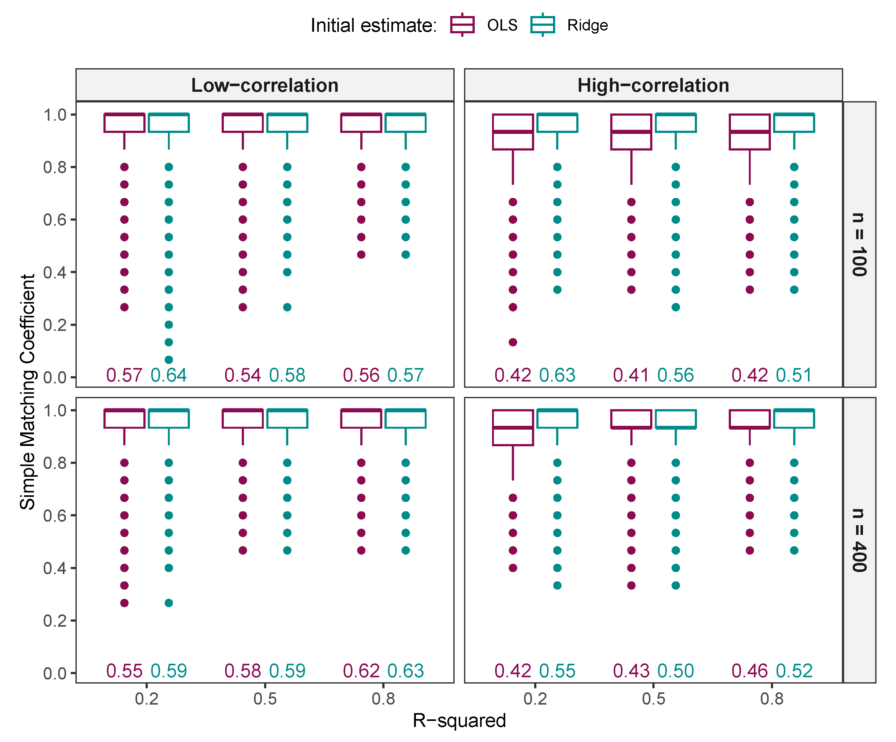
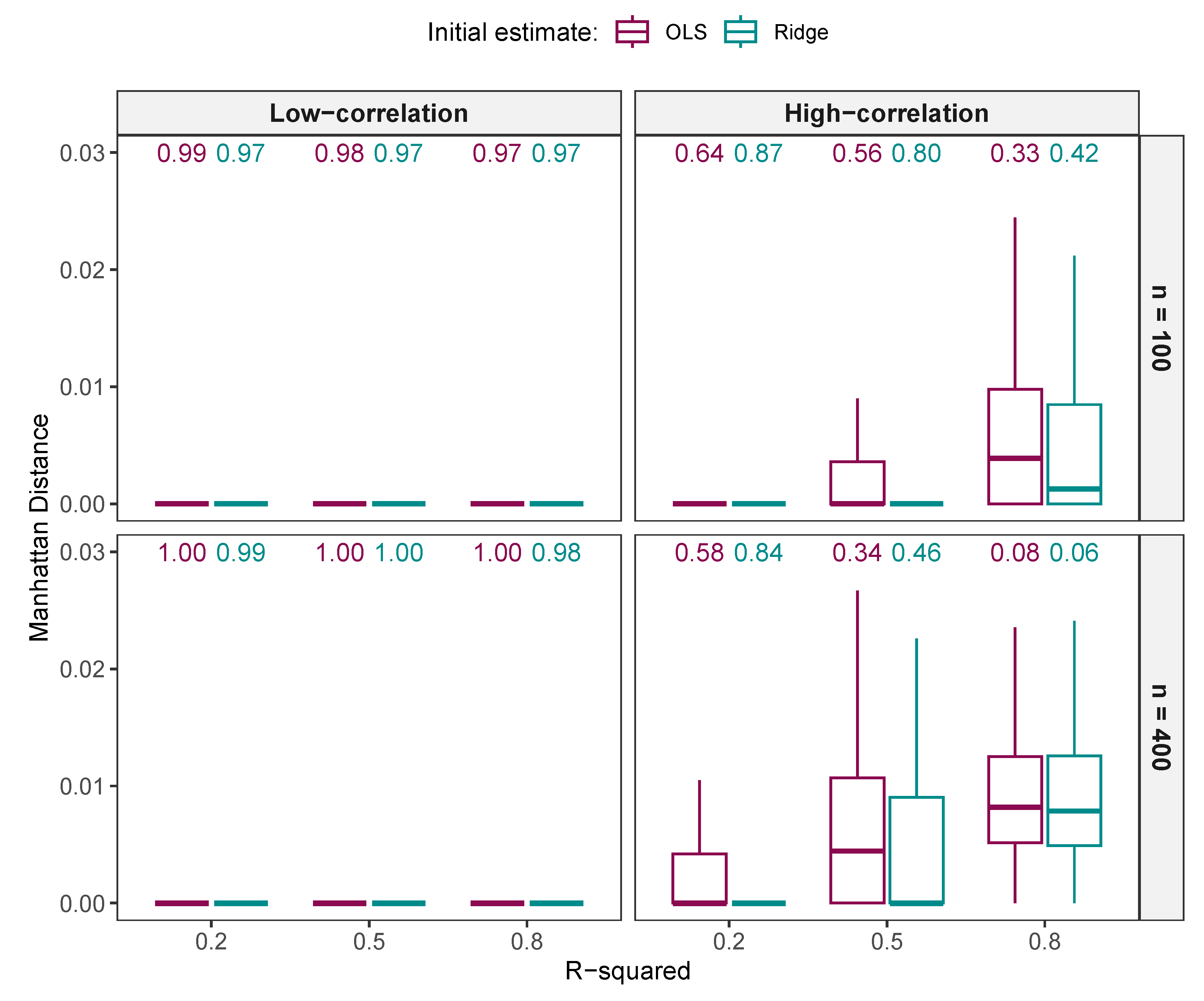
Figure 1 shows the distribution of SMC for variables selected by NNG and ALASSO ( γ = 1 ) using OLS and ridge initial estimates. The upper and lower panels display the results for small ( n = 100 ) and large ( n = 400 ) sample sizes, respectively, while the left and right panels show the results for low (C2) and high (C4) correlations, respectively. Various R 2 values ranging from low (20%) to high (80%) were evaluated. An SMC value of zero indicates no overlap in the selected variables, whereas a value of one indicates perfect agreement (see Section 2.3.1 for details). The proportion of replications in which SMC = 1 is also displayed for each scenario.
In low-correlation settings (left panel), an SMC of 1 was observed in nearly all replications, implying that both approaches consistently selected the same variables. However, in high-correlation settings (right panel), particularly with small sample sizes and low R 2 , the frequency with which SMC = 1 occurred decreased to approximately 93% with OLS initial estimates and 96% with ridge initial estimates (top right panel), indicating slightly lower agreement when OLS was used. Additionally, high-correlation settings resulted in more outlying SMC values than low-correlation settings, suggesting that in certain scenarios the two approaches differed substantially in the variables they selected.
Overall, ridge initial estimates improved similarity compared to OLS (top right panel) in high-correlation settings with low (20%) to moderate (50%) R 2 and small sample sizes, likely because ridge estimates are more stable than OLS estimates under these conditions. However, they reduced similarity when sample sizes were large and both correlation and R 2 were high, as indicated by a frequency of 0.90 compared to 0.99 for OLS (bottom right panel). Despite these differences, the similarity between the two approaches remained high, with a minimum SMC frequency of 90%.

Comparison of Variables Selected by NNG and ALASSO ( γ 1 )

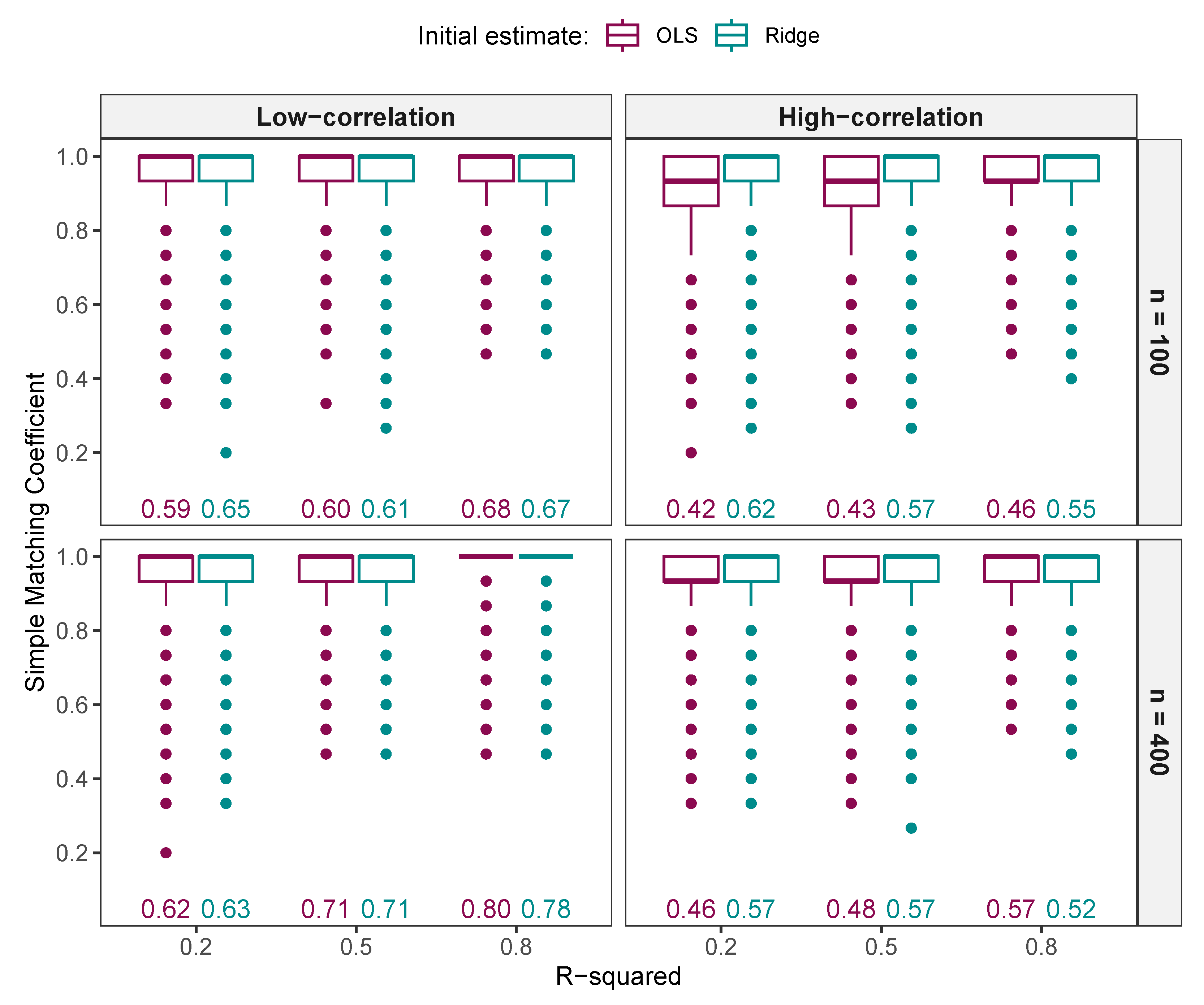
Figure 2 shows the distributions of SMC values for the variables selected by NNG and ALASSO ( γ = 2 ). In low-correlation settings, both methods selected the same set of variables (SMC = 1) in approximately 59% of replications using OLS initial estimates and 65% using ridge initial estimates under conditions of small sample size and low R 2 (top left panel). This similarity increased to approximately 80% with OLS and 78% with ridge when both the sample size and R 2 were high (bottom left panel).
In contrast, the similarity between NNG and ALASSO declined in high-correlation settings. Specifically, for small sample sizes and low R 2 (top right panel), the proportion of identical selections dropped from 59% (OLS) and 65% (ridge) in low-correlation settings to approximately 42% with OLS and 62% with ridge initial estimates. Similarity decreased further in large sample settings with high R 2 (bottom right panel), from 80% (OLS) and 78% (ridge) in low-correlation settings to 57% and 52%, respectively. Similar patterns were observed when NNG was compared with ALASSO ( γ = 0.5 ) (see Figure A1).
Overall, while NNG and ALASSO ( γ = 2 ) did not consistently select the same variables as NNG and ALASSO ( γ = 1 ), the level of similarity remained high in scenarios with large sample sizes, low correlations, and high R 2 values.

3.1.3. Comparison of FNR, FPR, and MCC

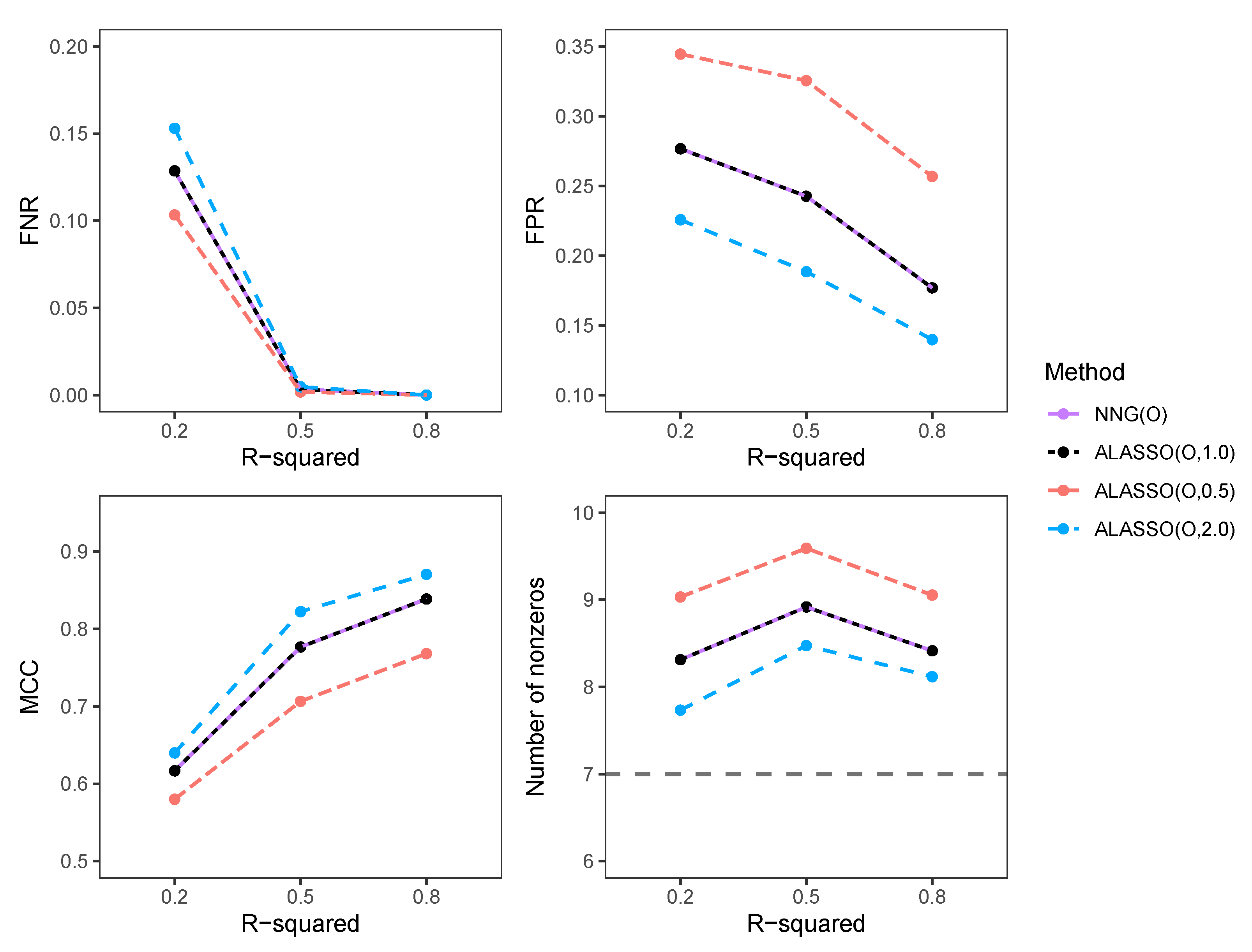
Figure 3 compares the FNR, FPR, and MCC for NNG and ALASSO ( γ = 0.5 , 1 , 2 ), using OLS as the initial estimator. The analysis was conducted under low-correlation settings with a sample size of n = 400 and varying R 2 values. The results for NNG and ALASSO ( γ = 1 ) were nearly identical across all R 2 values, as indicated by overlapping lines in the plots, suggesting that these methods can be used interchangeably under such conditions.
In moderate (0.5) and high (0.8) R 2 settings, all methods yielded similar FNR values, which were close to zero. However, under low- R 2 conditions, ALASSO ( γ = 2 ) exhibited a higher FNR, whereas ALASSO ( γ = 0.5 ) showed a lower FNR. NNG and ALASSO ( γ = 1 ) both produced intermediate FNRs (top left panel). This pattern suggests that when data contain limited information, ALASSO ( γ = 2 ) may be more likely to eliminate relevant variables, particularly those with weaker effects. This behavior is likely due to the larger weights assigned to small coefficients, as discussed in Section 2.4.3.
On the other hand, ALASSO ( γ = 0.5 ) had a higher FPR across low to high R 2 , whereas ALASSO ( γ = 2 ) had a lower FPR (top right panel). This suggests that ALASSO ( γ = 2 ) may be preferable when a simpler model is desired, as it tends to select models with fewer variables (bottom right panel).
The MCC values for all the approaches increased as R 2 increased, indicating improved ability to distinguish between signal and noise variables (bottom left panel). ALASSO ( γ = 0.5 ) was less effective in classifying variables, as evidenced by its lowest MCC values, which can be attributed to a higher FPR. In contrast, ALASSO ( γ = 2 ) achieved the highest MCC values, demonstrating superior performance in distinguishing between signal and noise variables. NNG and ALASSO ( γ = 1 ) showed intermediate performance, with MCC values falling between the extremes of ALASSO ( γ = 0.5 ) and ALASSO ( γ = 2 ).
In summary, ALASSO ( γ = 2 ) demonstrated superior performance in variable selection, especially when R 2 was moderate to high. Conversely, ALASSO ( γ = 0.5 ) was less effective because it selected a large number of noise variables, which negatively affected its overall performance, as indicated by the lower MCC values. NNG and ALASSO ( γ = 1 ) yielded intermediate results, performing reasonably well but not as effectively as ALASSO ( γ = 2 ). When OLS initial estimates were replaced with ridge estimates, similar patterns were observed even for small sample sizes with high correlations (Figure A2).

3.1.4. Comparison of Regression Estimates

In Section 3.1.2, we compared variables selected by NNG and ALASSO with different γ values. While both approaches may select the same variables, their estimated regression coefficients can differ. This section compares the regression estimates of NNG and ALASSO ( γ =   0.5 ,   1 ,   2 ) using MD. As described in Section 2.3.2, an MD of zero indicates that the estimates are identical in a given replication of a scenario. We also report the proportion of replications in which the MD equals zero for each scenario. A high proportion indicates that the methods produce identical estimates in many replications, while a low proportion suggests greater variability between the estimates.

Comparison of Regression Estimates from NNG and ALASSO ( γ = 1 )

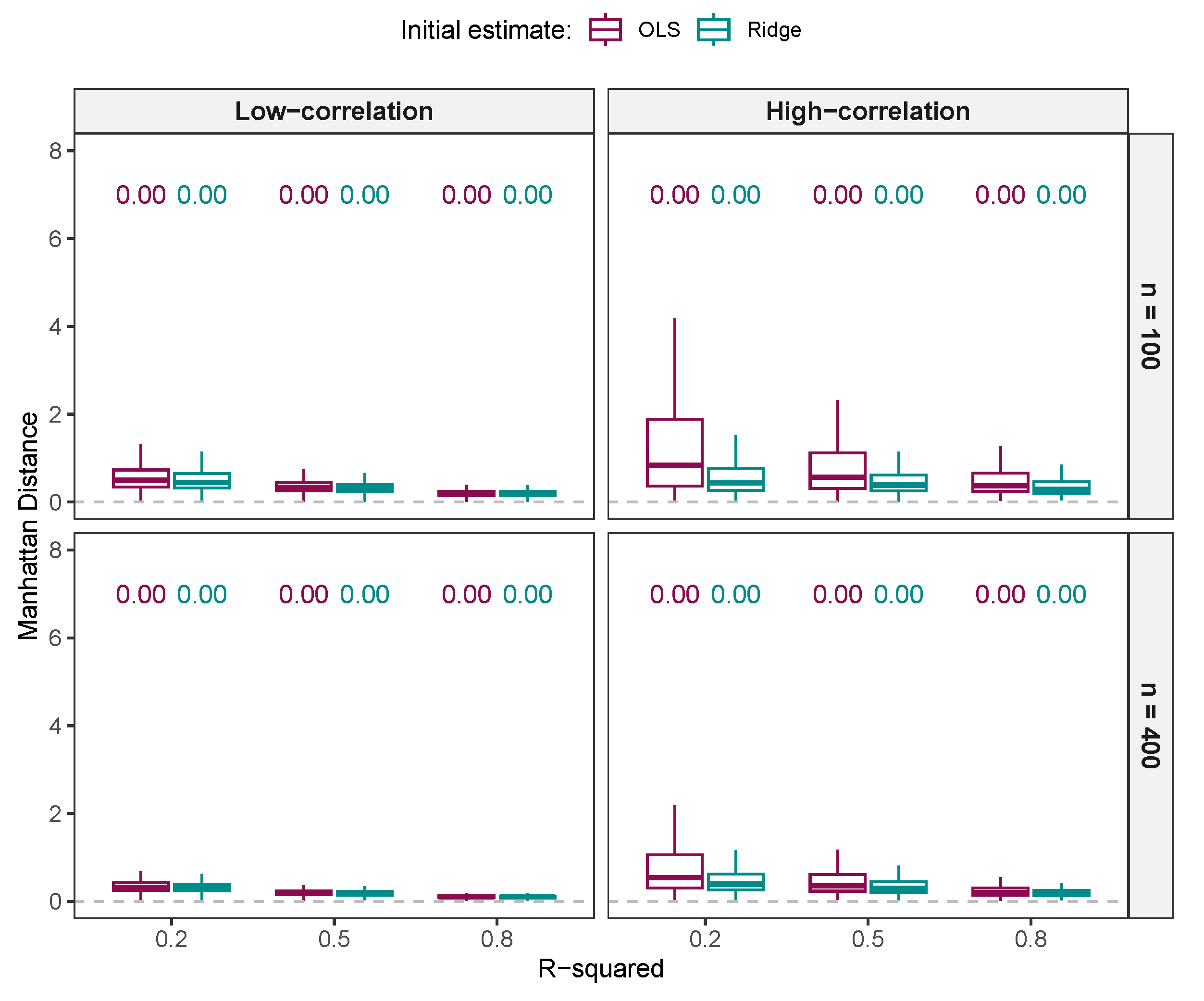
Figure 4 shows the distribution of MD between the regression estimates obtained from the two methods using both OLS and ridge initial estimates. In low-correlation settings (left panel), particularly with large sample sizes (bottom left panel), the regression estimates were identical (MD = 0) in nearly all replications. This high level of similarity aligns with the fact that the two approaches frequently selected the same variables (Figure 1), suggesting that the resulting models were approximately identical in most replications.
In high correlation settings (right panel), the similarity between the regression estimates decreased substantially depending on the choice of initial estimates. For instance, in scenarios with low R 2 , the proportion of replications yielding identical estimates was notably higher when ridge initial estimates were used (87% for small sample sizes and 84% for large sample sizes) than when OLS initial estimates were used (64% for small and 58% for large sample sizes). In some replications, particularly those with small sample sizes and with low R 2 , substantial differences in the regression estimates were observed, with MD values reaching as high as 23 (not shown in the plot). These discrepancies likely occurred because in high-correlation settings the two approaches were more prone to selecting different sets of variables (Figure 1, right panel). When the selected variables differ, the resulting regression estimates also differ, leading to higher MD values.
In summary, the results indicate that NNG and ALASSO ( γ = 1 ) produce almost identical regression estimates in low-correlation settings with large sample sizes, suggesting that the two methods yield similar models and may be used interchangeably in such cases. However, substantial differences emerge under high-correlation settings, particularly when R 2 is low. In these cases, ridge initial estimates tend to enhance similarity between the two methods.

Comparison of Regression Estimates from NNG and ALASSO ( γ 1 )

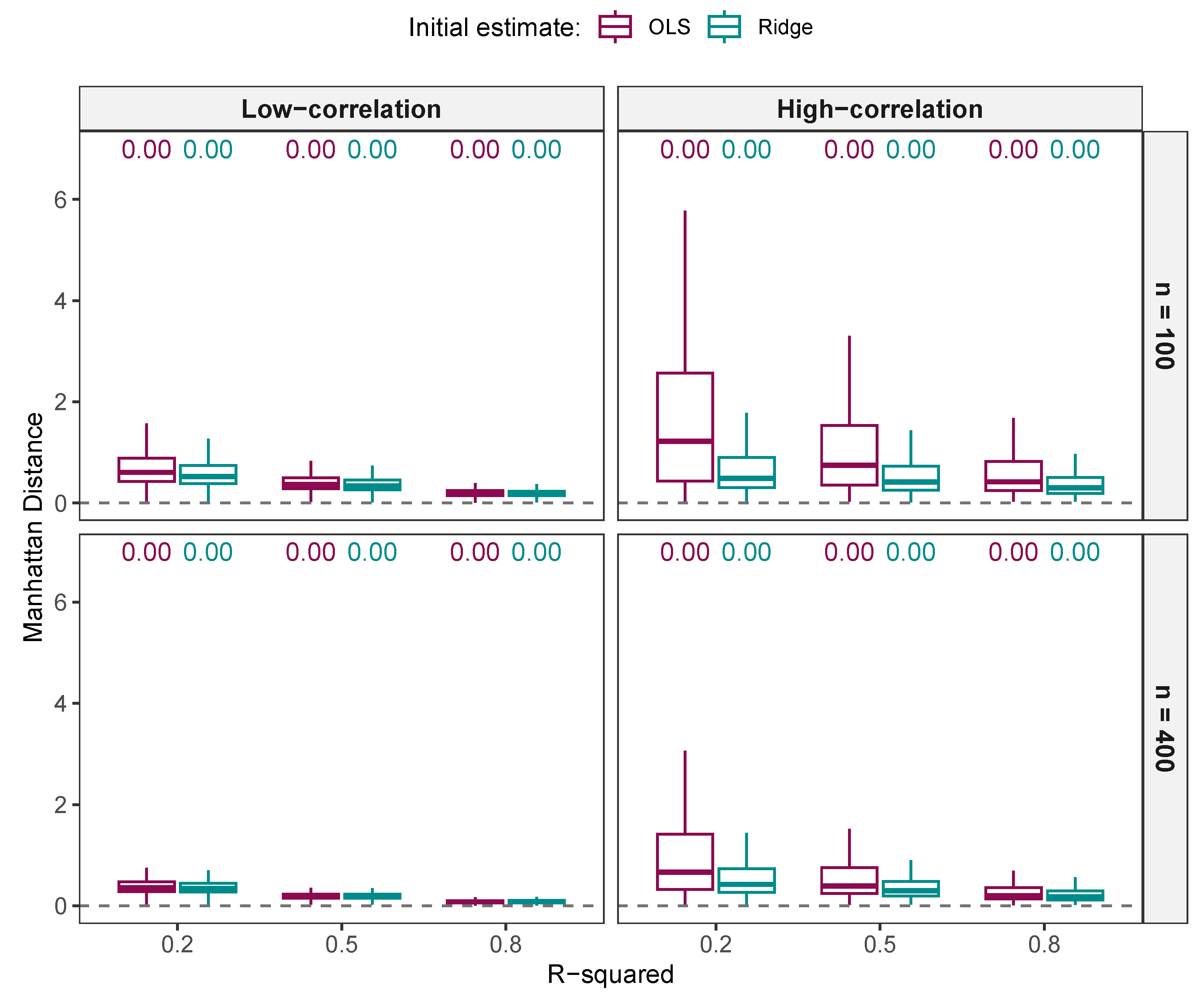
Figure 5 compares the regression estimates of NNG and ALASSO ( γ = 2 ). In all scenarios, the proportion of replications with MD equal to zero was zero, indicating that the regression estimates always differed. However, the magnitude of these differences varied depending on the correlation among variables, R 2 , sample size, and choice of initial estimates.
In low-correlation settings, particularly when R 2 was high (left panel), MD values were generally small and close to zero. This suggests that under these conditions, the regression estimates from both approaches were similar even though the selected variables only showed moderate overlap (Figure 2). The similarity likely resulted from the coefficient estimates for overlapping variables being similar across methods, while those for non-overlapping variables were close to zero.
Larger MD values were observed in high-correlation settings, especially with small sample sizes and low R 2 values (top right panel). These challenging conditions tend to reduce the accuracy of both coefficient estimation and variable selection, leading to substantial differences in the selected variables (Figure 2) and their corresponding regression estimates. The differences were more pronounced when OLS initial estimates were used, as this setting often results in estimates with high variance. Although NNG and ALASSO ( γ = 2 ) sometimes selected the same variables (Figure 2), their estimated coefficients differed, as reflected in the non-zero MD values.
A similar pattern was also observed when comparing NNG with ALASSO ( γ = 0.5 ) (Figure A3). Overall, NNG and ALASSO with γ 1 consistently differed in their regression estimates, with the degree of similarity influenced by the correlation structure, sample size, R 2 , and choice of initial estimates.

Comparison of the Prediction Performance of NNG and ALASSO ( γ =   0.5 ,   1 ,   2 )

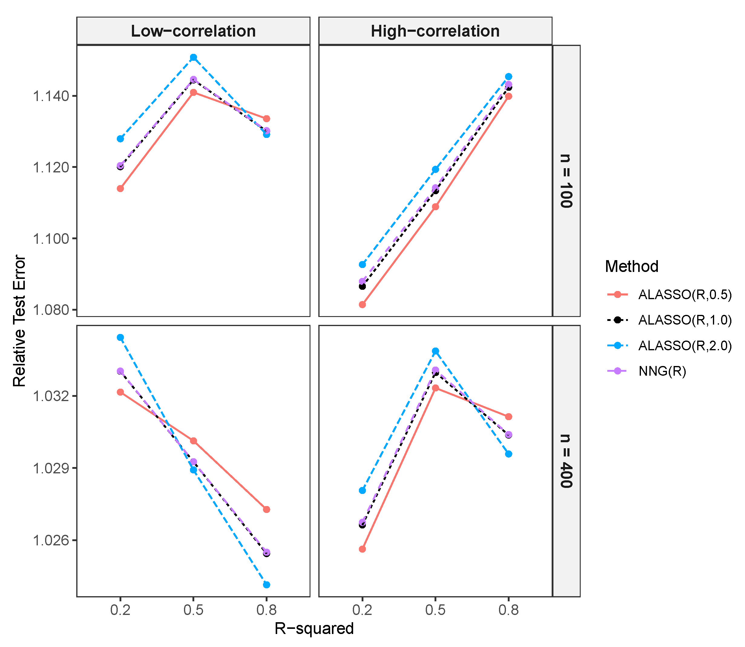
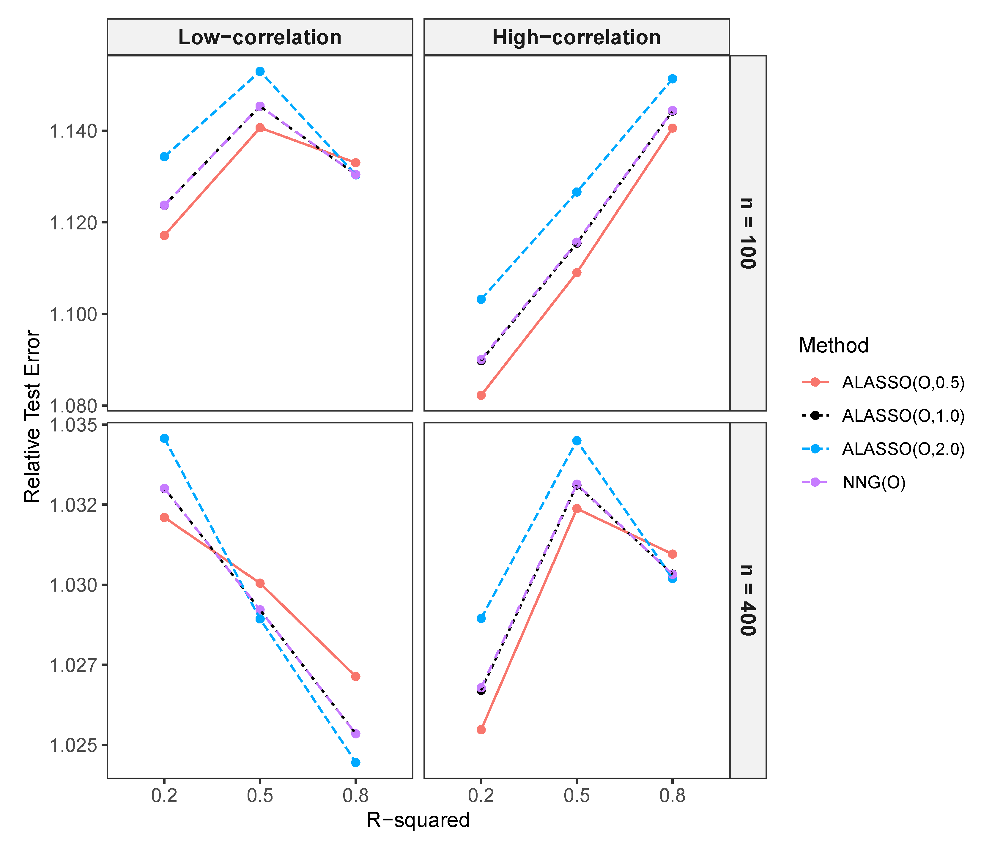
Figure 6 compares the prediction accuracy of NNG and ALASSO using the RTE metric. Results are shown for OLS initial estimates only, since the patterns were similar when ridge initial estimates were used (Figure A4). The prediction accuracy of NNG and ALASSO ( γ = 1 ) were approximately identical across all scenarios, as shown by the overlapping lines in the plot. This is not surprising given that the two methods selected identical models in nearly all replications, as described in Figure 1 and Figure 4.
ALASSO ( γ = 2 ) performed worse in settings with small sample sizes and low R 2 values (top left panel). It also performed poorly in small samples with high correlation, regardless of R 2 (top right panel). This poor performance is likely due to its high FNR in these settings (see Figure 3). However, it outperformed other approaches in scenarios with large sample sizes, low correlation, and moderate to large R 2 (bottom left panel), where it was more effective in minimizing both FPR and FNR (Figure 3).
ALASSO ( γ = 0.5 ) generally outperformed other approaches under challenging conditions such as small sample sizes, low R 2 values, and high correlation. Its tendency to select more variables and apply stronger shrinkage to moderate and large coefficients, as discussed in Section 2.4.4, likely contributed to its superior performance under these conditions.
In summary, NNG and ALASSO ( γ = 1 ) showed intermediate performance across different scenarios. ALASSO ( γ = 2 ) was more effective in scenarios with sufficient information, such as large sample sizes, low correlations, and high R 2 , where minimal shrinkage is often required. ALASSO ( γ = 0.5 ) performed better in more challenging conditions with insufficient information, such as small samples, low R 2 , and high correlation.

3.2. Simulation Results in High-Dimensional Settings

We repeated the analyses from the low-dimensional setting under high-dimensional settings to assess whether the results would remain consistent. To avoid complications posed by high correlation, only low-correlation settings were considered. The comparison of selected variables and corresponding regression estimates was restricted to NNG and ALASSO ( γ = 1 ), as earlier results in the low-dimensional setting showed that other ALASSO variants do not select the same variables as NNG. However, FNR, FPR, MCC, and RTE were reported for all methods. Ridge estimates were used as initial estimates for all approaches, as OLS estimates are not available in high-dimensional settings.

3.2.1. Comparison of Selected Variables and Regression Estimates for NNG and ALASSO ( γ = 1 ) in High-Dimensional Settings

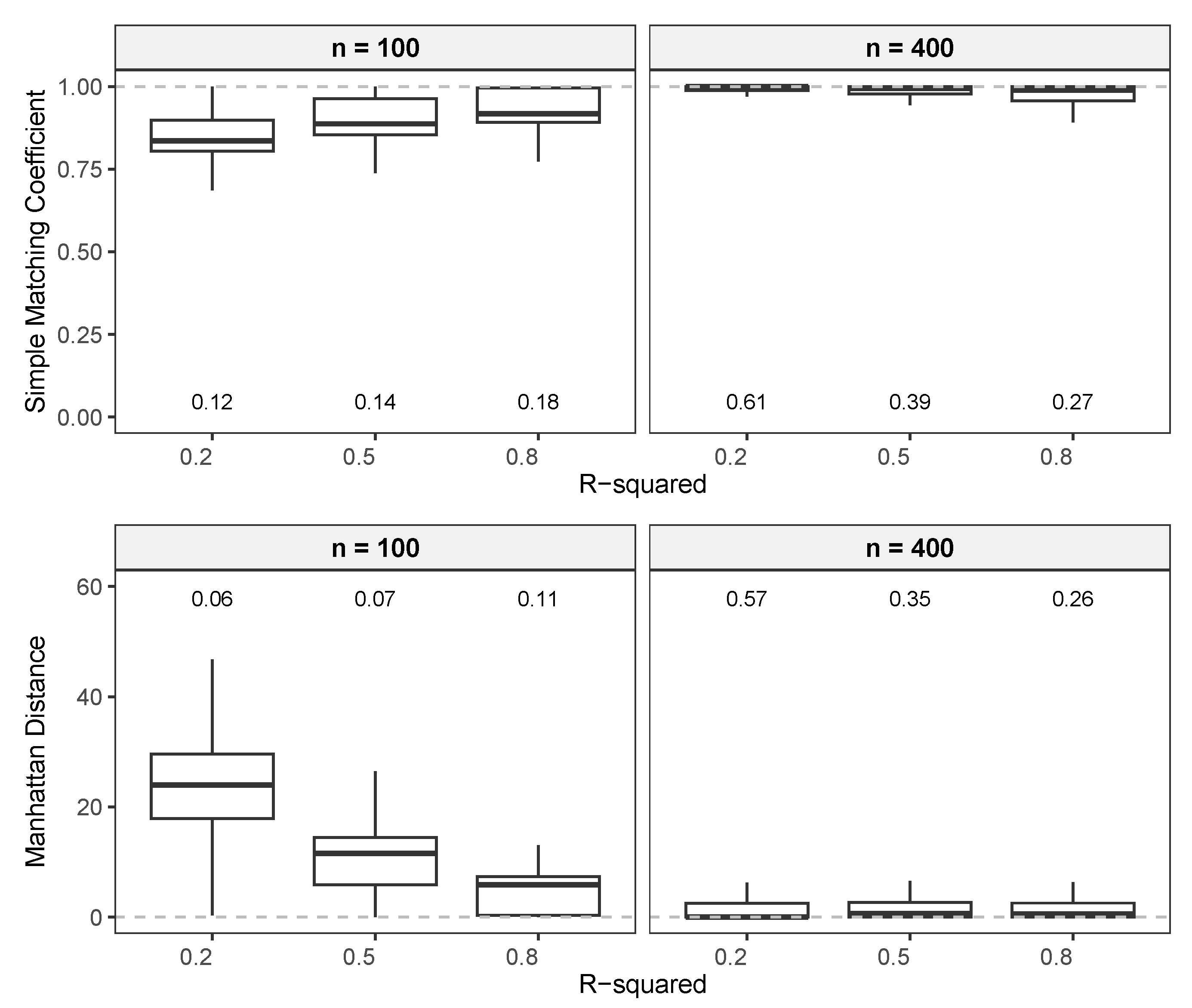
Figure A5 inAppendix A compares the variables selected by NNG and ALASSO ( γ = 1 ) using SMC (upper panel), while the lower panel shows the corresponding regression estimates compared using MD. Two key observations are evident. First, with a smaller sample size ( n = 100 ), the two methods selected different variables in most replications. This is reflected in the low proportion of SMC = 1, which range from 12% to 18%. As a result, their regression coefficients also differ considerably, especially in low R 2 scenarios, where MD values deviate substantially from zero (bottom left panel).
Second, with a larger sample size ( n = 400 ), similarity in the selected variables increases, with the proportion of replications with SMC = 1 ranging from 27% to 61% and most SMC values clustering near 1. Correspondingly, MD values are closer to zero (bottom right panel), indicating greater similarity between the selected models than in the small-sample settings.
These results are different from those in low-dimensional settings (Figure 1), where NNG and ALASSO ( γ = 1 ) yielded nearly identical sets of selected variables and coefficient estimates. The difference observed in high-dimensional settings likely stems from the difficulty of accurately estimating the signs of initial coefficients when many predictors are present and the sample size is small, which can cause the two methods to select different variables.

3.2.2. Comparison of FNR, FPR, MCC, and Number of Selected Variables in High-Dimensional Settings

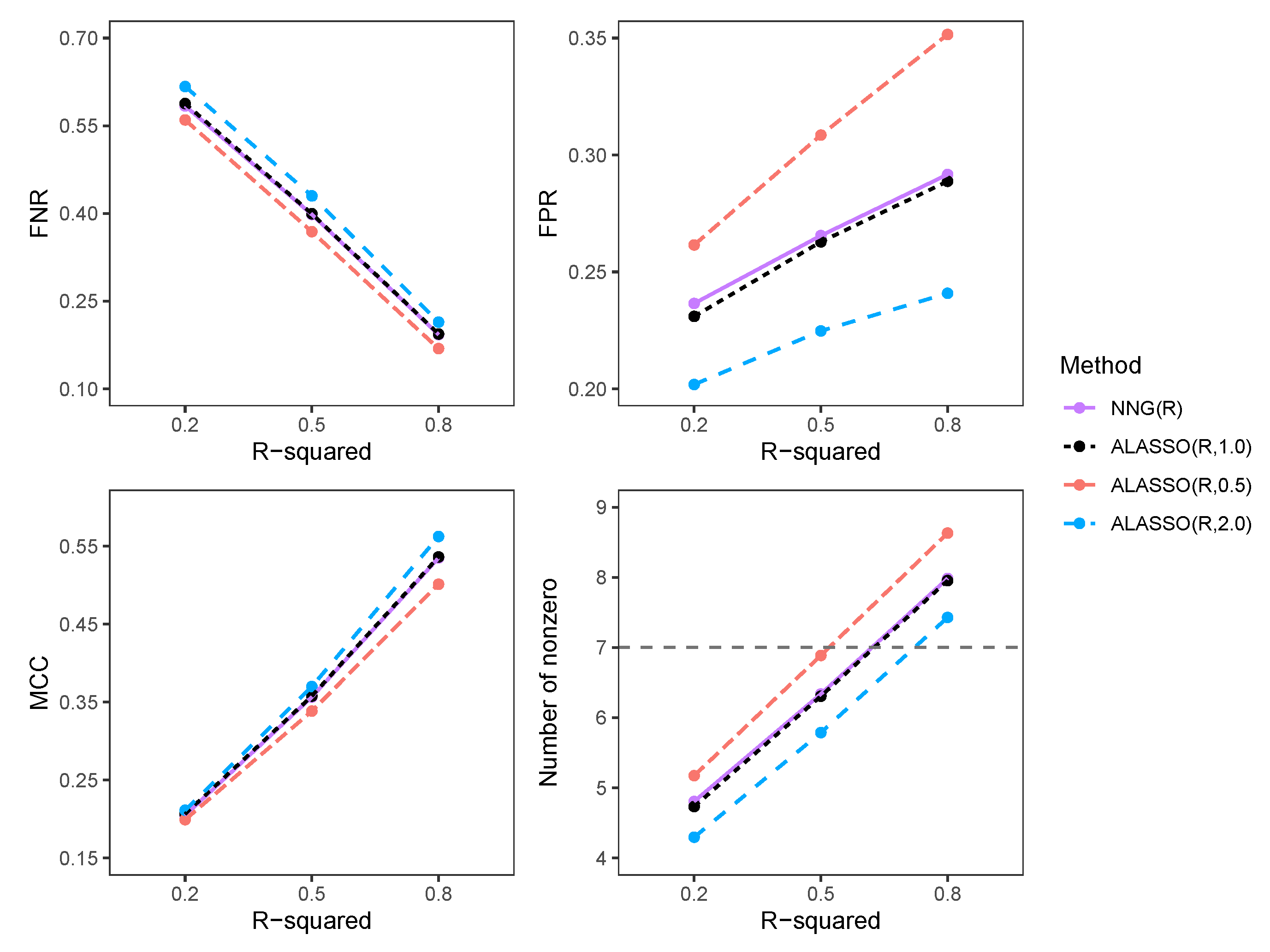
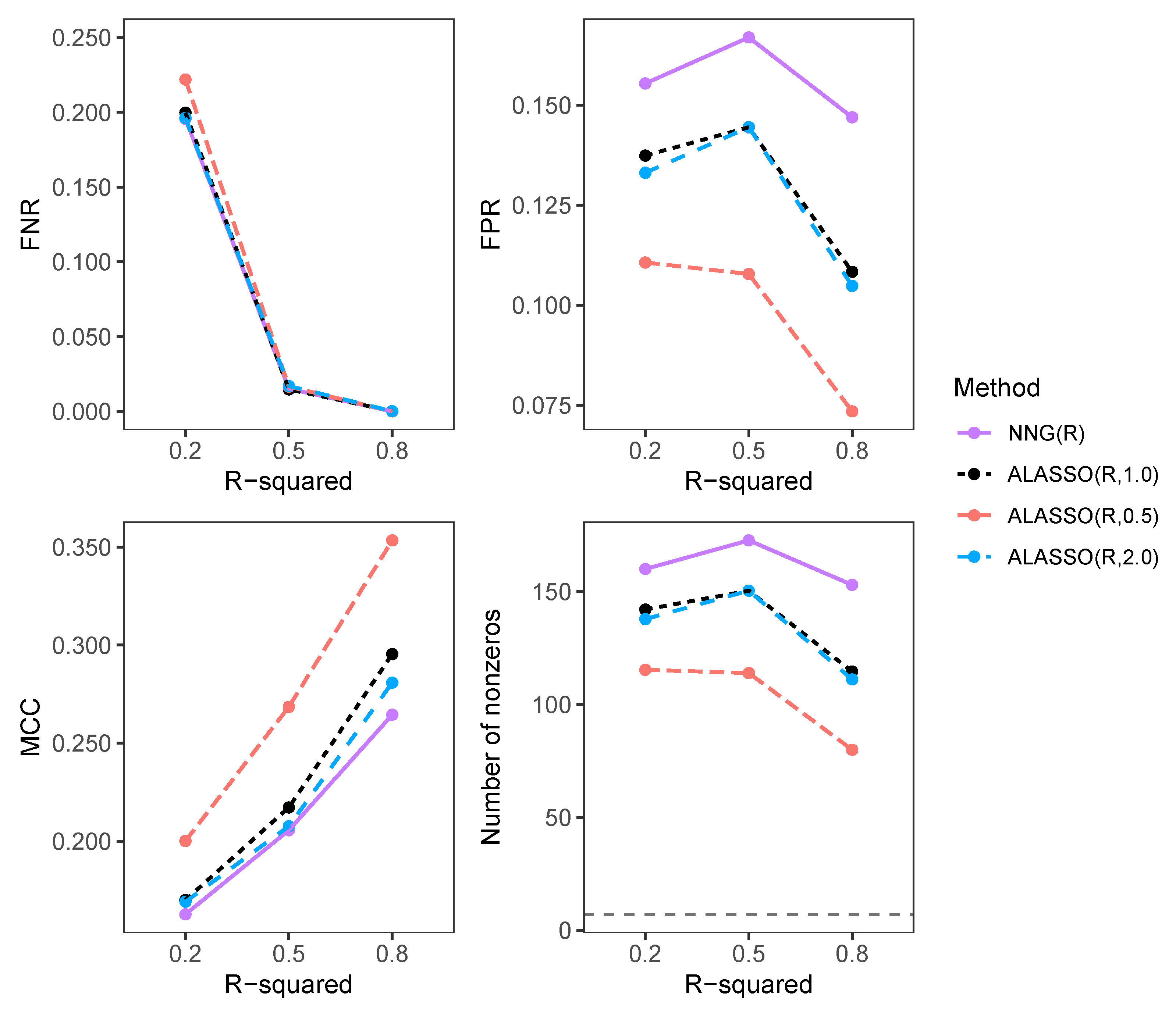
Figure 7 shows the values of FNR, FPR, and MCC along with the number of nonzero regression coefficients across different levels of R 2 . All methods show similar FNR values (top left panel), but their FPR values (top right panel) differ. In particular, NNG selected a large number of noise variables, while ALASSO ( γ = 0.5 ) selected fewer noise variables. This finding differs from the low-dimensional setting, where ALASSO ( γ = 0.5 ) selected many noise variables.
Unlike in the low-dimensional settings, where they performed similarly, NNG and ALASSO ( γ = 1 ) produced different results in high-dimensional settings. NNG showed inferior performance in variable selection, as reflected in lower MCC values (bottom left panel) and a larger number of selected variables (bottom right panel). ALASSO ( γ = 1 ) and ALASSO ( γ = 2 ) produced comparable results. Overall, all methods selected many noise variables, as seen in the total number of selected variables greatly exceeding the true number of signals (seven, indicated by the horizontal dashed line).

3.2.3. Comparison of Prediction Performance in High-Dimensional Settings

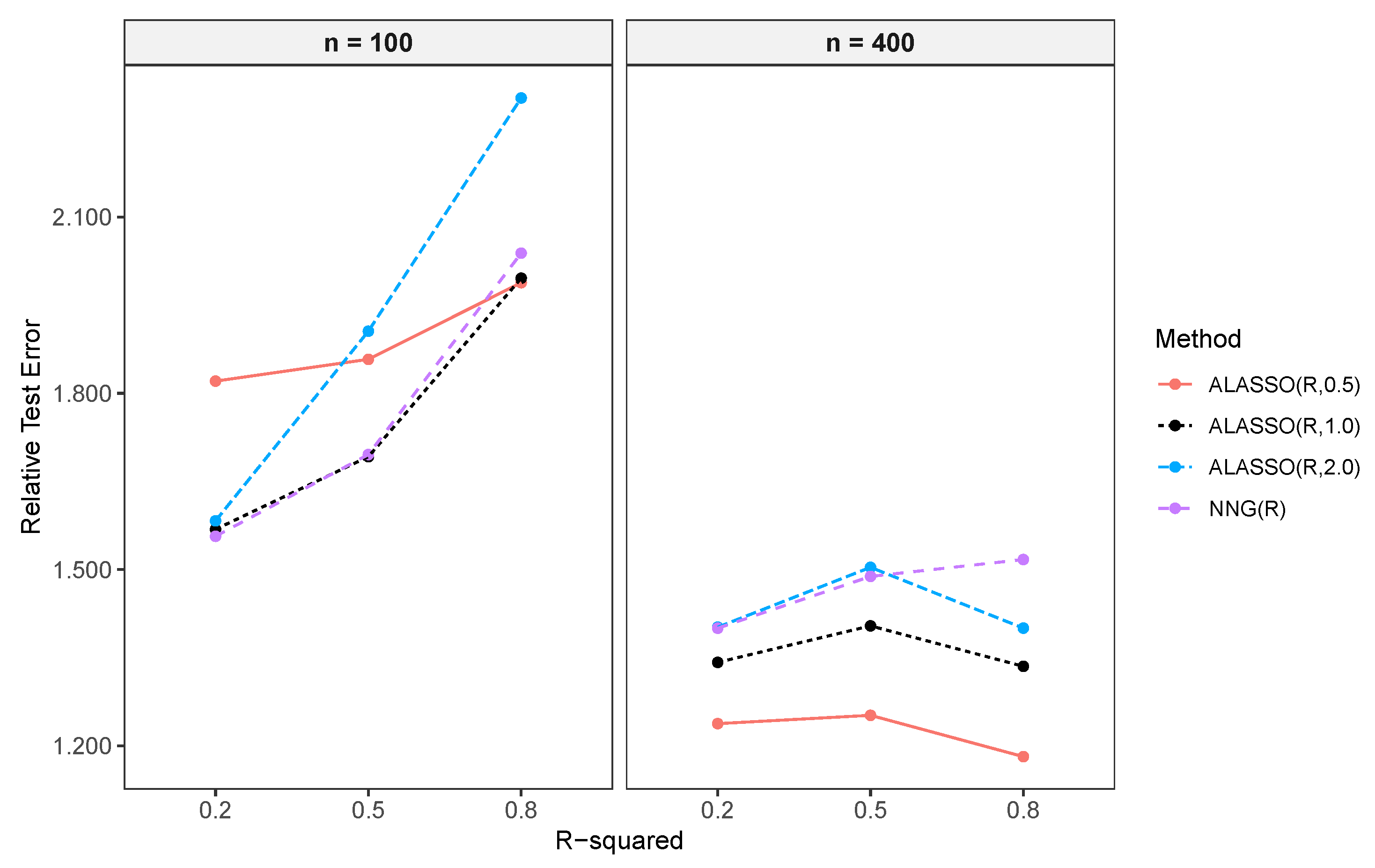
Figure A6 in Appendix A compares the prediction accuracy of NNG and ALASSO ( γ = 0.5 , 1 , 2 ) across different values of R 2 for both small ( n = 100 ) and large ( n = 400 ) sample sizes.
In the small-sample setting (left panel), NNG and ALASSO ( γ = 1 ) showed similar performance, and both generally outperformed ALASSO with γ = 0.5 and γ = 2 . ALASSO ( γ = 0.5 ) performed poorly at low R 2 values, while ALASSO ( γ = 2 ) performed worse at high R 2 values. These findings differ from the low-dimensional results (Figure 6), where ALASSO ( γ = 0.5 ) consistently outperformed the other approaches at low to moderate R 2 values.
In the large-sample setting (right panel), prediction accuracy improved for all methods, as RTE values were closer to 1. ALASSO ( γ = 0.5 ) consistently outperformed the other approaches regardless of R 2 , followed by ALASSO ( γ = 1 ). ALASSO ( γ = 2 ) and NNG performed similarly, although NNG was slightly worse at higher R 2 values, likely due to its tendency to select more noise variables (see Figure 7).

3.3. Real Data Examples

To strengthen the practical relevance of our study, we analyzed two real datasets: a high-dimensional gene expression dataset [41] and a low-dimensional prostate cancer dataset [42].

3.3.1. Gene Expression Data

The gene expression dataset includes 286 patients with lymph node-negative breast cancer, with a binary outcome indicating relapse ( n 1 = 107 ) or no relapse ( n 2 = 179 ) and 22,283 gene expression covariates. Table 6 compares the variables selected by NNG and ALASSO ( γ = 0.5 , 1 , 2 ) using ridge initial estimates. Both NNG and ALASSO ( γ = 1 ) selected the same 141 variables and their regression estimates were nearly identical, as indicated by an MD of 0.85, which is close to zero.
In contrast, ALASSO ( γ = 0.5 ) selected a larger number of variables (201) and produced regression estimates that differed substantially from those of NNG, as reflected by a large MD value of 24.17. ALASSO ( γ = 2 ) selected fewer variables (120) than all other approaches, with regression estimates that also deviated from those of NNG, as indicated by an MD of 11.39.
In this dataset, NNG and ALASSO ( γ = 1 ) produced similar models, aligning with observations from certain high-dimensional simulation settings.

3.3.2. Prostate Cancer Data

We further compared the methods using a prostate cancer dataset consisting of medical records from 97 male patients scheduled to undergo radical prostatectomy. The dataset includes eight clinical measurements used as covariates: log(cancer volume) ( x 1 ), seminal vesicle invasion ( x 2 ), log(prostate weight) ( x 3 ), age ( x 4 ), log(benign prostatic hyperplasia amount) ( x 5 ), log(capsular penetration) ( x 6 ), percentage of Gleason score 4 or 5 ( x 7 ), and Gleason score ( x 8 ). The response variable is the level of prostate-specific antigen (PSA).
Table A1 (Appendix A) shows the variables selected by NNG and ALASSO using OLS initial estimates. OLS was used because the predictors were moderately correlated, a condition under which OLS is often recommended. NNG and ALASSO ( γ = 1 ) selected the same seven variables, and their corresponding regression estimates were identical. In contrast, ALASSO ( γ = 2 ) selected a simpler model with only three variables, and its estimates differed from those of NNG. These results illustrate that ALASSO ( γ = 0.5 ) can produce a simpler model than ALASSO ( γ = 1 ) when the tuning parameter ( λ ) is substantially larger ( λ = 0.011 vs. 0.002).
Overall, all four models fit the data similarly, with adjusted R 2 values around 63%. In this case, ALASSO ( γ = 2 ) may be preferable because of its simplicity.

4. Discussion

In a simulation study conducted in both low- and high-dimensional settings, we investigated the similarities and differences between the models selected by NNG and ALASSO. There are two main distinctions between these approaches. First, NNG has a single tuning parameter ( λ ), whereas ALASSO has two ( λ and γ ). Second, NNG depends on both the sign and magnitude of the initial estimates, while ALASSO relies only on the magnitude.
In practice, using ALASSO requires deciding whether to fix γ (often set to 1) or to estimate it, a choice that can significantly influence model selection. In order to fairly compare ALASSO with NNG, we evaluated several values of γ . Our results show that NNG and ALASSO ( γ = 1 ) produce very similar models in low-dimensional settings. However, ALASSO’s flexibility through γ may offer advantages in certain cases. We also discuss applications from prior studies where NNG has been successfully used. We conclude by summarizing our findings and proposing several directions for future research.

4.1. NNG Versus ALASSO ( γ = 1 )

In our simulations, NNG and ALASSO ( γ = 1 ) performed quite similarly in low-dimensional settings with low correlation; they selected the same variables in most cases (Figure 1, left panel), and produced nearly identical regression estimates (Figure 4, left panel) and prediction accuracy (Figure 6, left panel). This high similarity likely stems from the low variability in initial estimates, which reduces the likelihood of incorrect signs, particularly for moderate and strong effects. These findings support theoretical results showing that NNG can be viewed as equivalent to ALASSO ( γ = 1 ) [6]. Moreover, in orthonormal settings, the two methods produced identical results, as demonstrated in Section 2.4.4, which is consistent with existing theoretical results [20]. These findings suggest that in low-dimensional settings with low correlation, sufficiently large sample sizes, and moderate to high R 2 values, the two approaches often select the same model and may be used interchangeably.
However, in settings with high correlation, especially when combined with small samples and low R 2 values, the similarity between the two approaches decreased. The same was found in high-dimensional settings. In these cases, the initial estimates tend to have high variability; this increases the chance of assigning incorrect signs to variables with weak effects, which can lead to different sets of selected variables, as shown in Section 3.1.1. The predictive performance of NNG and ALASSO under moderate and low SNR has been compared in previous studies, which found that ALASSO often outperformed NNG [6]. This agrees with our findings and highlights the advantage of ALASSO’s γ parameter, which together with λ controls the amount of shrinkage applied to the regression coefficients.
In general, NNG and ALASSO ( γ = 1 ) produced nearly identical models under favorable conditions (low correlation, large samples, and moderate to high R 2 ) but produced different models when correlation was high, samples were small, and R 2 was low as well as in high-dimensional settings.

4.2. NNG Versus ALASSO ( γ 1 )

We compared the results of NNG, ALASSO ( γ = 0.5 ), and ALASSO ( γ = 2 ) and observed notable differences in selected variables, particularly in low-dimensional settings with high correlation (Figure 2). Additionally, their regression estimates (Figure 5) and prediction accuracy (Figure 6 and Figure A4) differed across all scenarios. These differences are partially attributable to the γ parameter, which controls the weights assigned to covariates, as demonstrated in Section 2.4.3, thereby influencing variable selection (Figure 3). Our findings agree with previous results showing that ALASSO’s performance depends critically on the value of γ (Table 1 in [6]). Specifically, ALASSO ( γ = 2 ) selected a higher proportion of signal variables and fewer noise variables than ALASSO ( γ = 1 ).
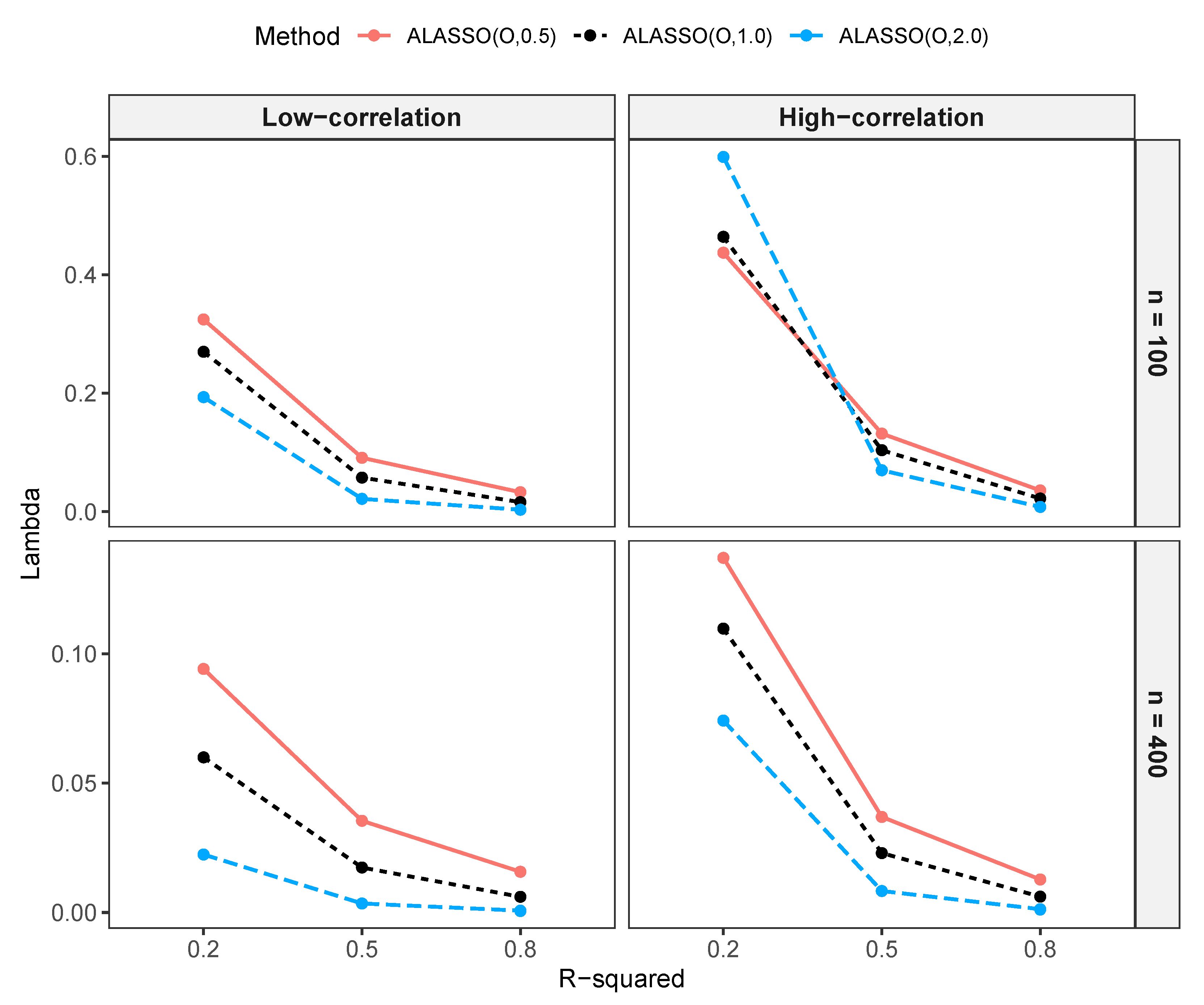
In low-dimensional settings, ALASSO ( γ = 2 ) selected simpler models than ALASSO ( γ = 0.5 ). This occurs because covariates with initial estimates near zero are assigned larger adaptive weights, resulting in stronger shrinkage (Table 3) and consequently in a lower FPR (Figure 3). In contrast, ALASSO ( γ = 0.5 ) requires a larger tuning parameter to achieve similar levels of sparsity (Figure A7), which can lead to overshrinkage of moderate to large effects. To prevent this, a smaller tuning parameter is typically used, leading to models with higher FPR (Figure 3), which aligns with previous findings [6]. As γ approaches zero, the adaptive weights converge to one, in which case ALASSO increasingly resembles the standard lasso method. This tends to select more variables, including noise, but may improve predictive performance when the SNR is low to moderate.
In high-dimensional settings, ALASSO ( γ = 0.5 ) outperformed the other ALASSO variants and NNG by selecting simpler models with superior predictive accuracy, suggesting that its penalty is more effective than those of ALASSO ( γ = 1 ) and ALASSO ( γ = 2 ). These results underscore the importance of jointly tuning both γ and λ in order to balance sparsity, variable selection accuracy, and predictive performance. A suboptimal choice of γ may lead to models that erroneously exclude relevant variables or include excessive noise, thereby compromising both interpretability and prediction accuracy.

4.3. When to Choose NNG over ALASSO

In our simulation study, NNG and ALASSO ( γ = 1 ) produced very similar results in low-dimensional settings, raising the question of whether NNG is necessary, given its sensitivity to the sign of the initial estimates and that this issue does not affect ALASSO. In such settings with low correlation, the two methods performed comparably (see Figure 3 and Figure 6) and can be used interchangeably.
However, their performance may differ in settings with high correlation, small sample sizes, and low R 2 values as well as in high-dimensional settings, with ALASSO ( γ = 1 ) generally proving more reliable. This is because the likelihood of incorrect signs in the initial estimates increases, particularly for variables with weak effects. Because ALASSO depends only on the magnitude of the initial estimates, it can adjust for incorrect signs if necessary, as demonstrated in Section 3.1.1. Despite this, both methods can become unreliable when the sample size is small or R 2 is low due to the high uncertainty in estimating tuning parameters and initial estimates. For this reason, researchers have argued that penalized regression methods should be used only when sufficient information is available in the data [28].
Here, we argue that models producing initial estimates with reversed signs can be misleading [19] and are not appropriate for generating initial estimates. As such, analysts must carefully select appropriate methods for obtaining initial estimates. For example, in high-correlation settings, ridge estimates are preferable to OLS estimates because of their stability [6], which may lead NNG and ALASSO ( γ = 1 ) to produce similar models, as observed in our study. In situations where the data provide limited information or the effects of interest are fairly small, distinguishing between noise and signal variables becomes challenging. In such cases, the appropriateness of using any analysis strategy may be questionable, as it can produce misleading results and waste valuable resources [43]. A more appropriate approach may be to summarize the data descriptively and recommend conducting a new and more informative study.
Although ALASSO is flexible, there are situations where NNG may be more appropriate, which are beyond the scope of this paper. For instance, if prior knowledge suggests that the signs of the initial estimates are meaningful and should be preserved, NNG can be used to align with these constraints. Similarly, when strictly non-negative shrinkage factors are required, such as for structurally grouped variables, e.g., dummy variables for multilevel categorical covariates [44] or basis expansions for continuous predictors [45,46,47], NNG provides a straightforward solution. In these cases, NNG’s non-negative shrinkage helps to maintain the direction of associations and avoids distorting the relationship between covariates and the outcome.
In contrast, ALASSO’s flexibility comes with added complexity, especially in choosing the tuning parameter γ . Analysts unfamiliar with how to select this parameter may have difficulty identifying an appropriate value, which can lead to suboptimal performance, as demonstrated in our study.

5. Conclusions

This study evaluated the performance of NNG and ALASSO across a range of scenarios in both low- and high-dimensional settings, with a focus on variable selection, regression estimates, and prediction accuracy. Under favorable conditions, such as low-dimensional settings with large sample sizes and moderate to high R 2 , both NNG and ALASSO ( γ = 1 ) performed similarly. In such cases, either method may be used. However, differences emerged in more challenging scenarios, including small sample sizes, low R 2 , high correlation, and high-dimensional settings. In these contexts, the signs of the initial estimates are less reliable, and ALASSO ( γ = 1 ) is preferable due to its insensitivity to sign errors and its ability to adjust for them. Overall, ALASSO ( γ = 1 ) appears to be a more robust choice than NNG for general use, as it tends to yield results that are comparable to or better than those of NNG while avoiding the limitations associated with NNG’s dependence on the sign of initial estimates.
We also explored how varying the γ parameter in ALASSO influences model performance and its similarity to NNG. When γ 1 , the overlap between the variables selected by ALASSO and NNG decreased even under favorable conditions, underscoring the important role of γ in ALASSO’s performance. Specifically, ALASSO ( γ = 2 ) performed best in low-dimensional settings with low correlation and high R 2 , where it selected simpler models with better accuracy than NNG and the other ALASSO variants. Conversely, ALASSO ( γ = 0.5 ) was more effective in challenging conditions such as high-dimensional settings or high correlation, where strong shrinkage is often beneficial. Thus, the γ parameter allows ALASSO to adapt its level of shrinkage to the complexity of the problem. However, the optimal value is typically unknown and must be specified or estimated in practice, for example through two-dimensional cross-validation, which can increase instability, especially with small samples or in highly correlated settings.
Lastly, while both NNG and ALASSO are suitable for data analysis, selecting an appropriate γ in ALASSO provides flexibility for handling more complex scenarios. In our simulation studies, ALASSO produced results that were either superior to or comparable with those of NNG. Therefore, we found no advantage of NNG over ALASSO, which may explain ALASSO’s growing popularity. These findings suggest that ALASSO is not only a viable alternative to NNG but also a more versatile and practically effective method for a wide range of regression problems.

6. Directions for Future Research

The choice of initial estimates plays a crucial role in the performance of both NNG and ALASSO [6,13]. This study considered only OLS and ridge estimates. Future research should investigate alternative options such as those derived from the lasso or elastic net in order to better understand how different initializations influence model performance.
In addition, we did not examine the robustness of NNG and ALASSO to violations of standard model assumptions, including heteroskedasticity and non-normal error distributions. This was a deliberate choice to allow for a clear and focused comparison of these methods under controlled conditions, with the aim of understanding their strengths and weaknesses when standard model assumptions are met. Assessing their performance under such conditions could shed light on their reliability in more realistic or applied settings. Our simulations also did not include interaction terms or nonlinear transformations of continuous covariates; extending the analysis to these more complex data-generating mechanisms would help to assess the methods’ adaptability to non-additive effects and nonlinear relationships, which are often encountered in practice. In ongoing work, we are also investigating extensions of these approaches to the selection of functional forms, particularly through the use of fractional polynomials.
Furthermore, both NNG and ALASSO have been extended to generalized linear models and survival models. Future work should assess whether our findings generalize to these broader settings. Finally, comparing the resulting regression estimates from NNG and ALASSO with those from other penalized regression approaches such as the elastic net may offer further insights into the their similarities.

Supplementary Materials

The following supporting information can be downloaded at: https://www.mdpi.com/article/10.3390/stats8030070/s1. Table S1. A summary of the simulation design following the ADEMP structure is available from Kipruto and Sauerbrei [14].

Author Contributions

Conceptualization, E.K. and W.S.; software, E.K.; data analysis, E.K.; writing—original draft preparation, E.K. and W.S.; writing—review and editing, E.K. and W.S. All authors have read and agreed to the published version of the manuscript.

Funding

This research was funded by the German Research Foundation (DFG), grant number SA580/10-3 to WS; see https://www.dfg.de/en/ (accessed on 5 July 2025) for more information.

Institutional Review Board Statement

Not applicable.

Informed Consent Statement

Not applicable.

Data Availability Statement

The code used to generate the datasets analyzed in the simulation study will be made available in a public repository at https://github.com/EdwinKipruto/Garrote_vs_AdaptiveLasso. This repository will also contain the gene expression and prostate cancer datasets analyzed in our study.

Acknowledgments

The authors gratefully acknowledge Milena Schwotzer and Sarah Hag-Yahia (Medical Center—University of Freiburg, Germany) for their invaluable administrative support. We acknowledge support by the Open Access Publication Fund of the University of Freiburg.

Conflicts of Interest

The authors declare no conflicts of interest; the funders had no role in the design of the study, in the collection, analysis, or interpretation of data, in the writing of the manuscript, or in the decision to publish the results.

Abbreviations

The following abbreviations are used in this manuscript:
AICAkaike information criterion
ALASSOAdaptive lasso
ALASSO( a , γ )Adaptive lasso using initial estimates from a (e.g., OLS or ridge) and γ > 0 .
BICBayesian information criterion
CVCross-validation
FNRFalse negative rate
FPRFalse positive rate
MCCMatthews correlation coefficient
MCSEMonte Carlo standard error
MDManhattan distance
MEModel error
MSEMean squared error
NNGNon-negative garrote
NNG(O)Non-negative garrote with OLS initial estimates
NNG(R)Non-negative garrote with ridge initial estimates
OLSOrdinary least squares
R 2 Coefficient of determination
RTERelative test error
SMCSimple matching coefficient

Appendix A. Results

Table A1. Prostate cancer data. Regression coefficients of NNG and ALASSO using OLS initial estimates. Both NNG and ALASSO (1) selected the same model. ‘-’ denotes a zero coefficient.
VariableNNGALASSO (1)ALASSO (0.5)ALASSO (2)
x 1 0.650.650.620.64
x 2 0.290.290.250.24
x 3 0.260.260.240.24
x 4 −0.13−0.13−0.08-
x 5 0.120.120.10-
x 6 −0.09−0.09--
x 7 0.110.110.06-
x 8 ----
Adj. R 2 0.640.640.630.62
λ 0.00160.00160.011210.0028
Figure A1. Low-dimensional data. Boxplots comparing SMC for variables selected by NNG and ALASSO ( γ = 0.5 ) using OLS and ridge initial estimates. The upper and lower panels display results for small ( n = 100 ) and large ( n = 400 ) sample sizes, respectively. The left and right panels shows results for low and high correlation, respectively. The plots show the proportion of 10,000 replications in which SMC = 1 across various R 2 values.
Stats 08 00070 g0a1
Figure A2. Low-dimensional data. Comparison of average FNR, FPR, MCC, and the number of variables selected for by NNG and ALASSO (with γ values of 0.5, 1, and 2) using ridge initial estimates in high-correlation settings with a small sample size ( n = 100 ). The results for NNG and ALASSO ( γ = 1 ) are almost identical, as shown by the overlapping lines. The horizontal dashed line in the bottom right panel indicates the number of signal variables (7).
Stats 08 00070 g0a2
Figure A3. Low-dimensional data. Boxplots comparing the Manhattan distance of regression estimates for NNG and ALASSO ( γ = 0.5 ) using OLS and ridge initial estimates. The plots display results for small sample sizes (upper panel) and large sample sizes (lower panel), with low correlation (left panel) and high correlation (right panel) across various R 2 values. The plots also show the proportion of 10,000 replications with a Manhattan distance of zero. Outlying distances are not shown.
Stats 08 00070 g0a3
Figure A4. Low-dimensional data. Comparison of prediction accuracy assessed using the RTE metric for NNG and ALASSO with different values of γ (0.5, 1, and 2). The plots display results for small sample sizes (upper panel) and large sample sizes (lower panel) with low correlation (left panel) and high correlation (right panel) across various R 2 values. The performance of NNG and ALASSO ( γ = 1 ) is nearly identical, as shown by the overlapping lines. OLS initial estimates were used in all approaches. Bars with a size of one standard error were added, but are not visible due to the small standard errors.
Stats 08 00070 g0a4
Figure A5. Low-dimensional data. Comparison of variables selected by NNG and ALASSO ( γ = 1 ) using SMC (upper panel) along with their corresponding regression coefficients assessed through MD (lower panel) in a high-dimensional setting. The left panel displays results for n = 100 , while the right panel shows results for n = 400 , both under low correlation (C2) and p = 1000 variables. Ridge initial estimates were used in both approaches. Outlying values are not shown.
Stats 08 00070 g0a5
Figure A6. High-dimensional data. Comparison of prediction accuracy assessed using the RTE metric for NNG and ALASSO with different values of γ (0.5, 1, and 2). The plots display results for sample sizes n = 100 (left panel) and n = 400 (right panel) with low correlation (C2) across various R 2 values. Bars with a size of one standard error were added, but are not visible due to the small standard errors resulting from the large number of simulation repetitions.
Stats 08 00070 g0a6
Figure A7. Low-dimensional data. Average λ values for ALASSO for different γ values across various R 2 levels. The plots display results for small sample sizes (upper panels) and large sample sizes (lower panels) with low correlation (left panels) and high correlation (right panels) in low-dimensional settings.
Stats 08 00070 g0a7

References

  1. Heinze, G.; Wallisch, C.; Dunkler, D. Variable selection—a review and recommendations for the practicing statistician. Biom. J. 2018, 60, 431–449. [Google Scholar] [CrossRef]
  2. Sauerbrei, W.; Perperoglou, A.; Schmid, M.; Abrahamowicz, M.; Becher, H.; Binder, H.; Dunkler, D.; Harrell, F.E.; Royston, P.; Heinze, G. On behalf of TG2 of the STRATOS initiative. State of the art in selection of variables and functional forms in multivariable analysis—Outstanding issues. Diagn. Progn. Res. 2020, 4, 1–8. [Google Scholar] [CrossRef]
  3. Harrell, F.E. Regression Modeling Strategies: With Applications to Linear Models, Logistic Regression, and Survival Analysis; Springer: New York, NY, USA, 2015. [Google Scholar]
  4. James, G.; Witten, D.; Hastie, T.; Tibshirani, R. An Introduction to Statistical Learning: With Applications in R; Springer: New York, NY, USA, 2013; Volume 103. [Google Scholar]
  5. Hastie, T.; Tibshirani, R.; Friedman, J.H. The Elements of Statistical Learning: Data Mining, Inference, and Prediction; Springer: New York, NY, USA, 2009; Volume 2, pp. 1–758. [Google Scholar]
  6. Zou, H. The adaptive lasso and its oracle properties. J. Am. Stat. Assoc. 2006, 101, 1418–1429. [Google Scholar] [CrossRef]
  7. Breiman, L. Better subset regression using the nonnegative garrote. Technometrics 1995, 37, 373–384. [Google Scholar] [CrossRef]
  8. Huang, J.; Ma, S.; Zhang, C.H. Adaptive lasso for sparse high-dimensional regression models. Stat. Sin. 2008, 18, 1603–1618. [Google Scholar]
  9. Makalic, E.; Schmidt, D.F. Logistic regression with the nonnegative garrote. In AI 2011: Advances in Artificial Intelligence; Walsh, T., Ed.; Springer: Berlin/Heidelberg, Germany, 2011; pp. 82–91. [Google Scholar]
  10. Antoniadis, A.; Gijbels, I.; Verhasselt, A. Variable selection in additive models using P-splines. Technometrics 2012, 54, 425–438. [Google Scholar] [CrossRef]
  11. Gregorich, M.; Kammer, M.; Mischak, H.; Heinze, G. Prediction modeling with many correlated and zero-inflated predictors: Assessing the nonnegative garrote approach. Stat. Med. 2025, 44, e70062. [Google Scholar] [CrossRef]
  12. Meinshausen, N. Relaxed lasso. Comput. Stat. Data Anal. 2007, 52, 374–393. [Google Scholar] [CrossRef]
  13. Yuan, M.; Lin, Y. On the non-negative garrotte estimator. J. R. Stat. Soc. Ser. B Stat. Methodol. 2007, 69, 143–161. [Google Scholar] [CrossRef]
  14. Kipruto, E.; Sauerbrei, W. Comparison of variable selection procedures and investigation of the role of shrinkage in linear regression-protocol of a simulation study in low-dimensional data. PLoS ONE 2022, 17, e0271240. [Google Scholar] [CrossRef]
  15. Kipruto, E.; Sauerbrei, W. Evaluating prediction performance: A simulation study comparing penalized and classical variable selection methods in low-dimensional data. Appl. Sci. 2025, 15, 7443. [Google Scholar] [CrossRef]
  16. Tibshirani, R. Regression shrinkage and selection via the lasso. J. R. Stat. Soc. Ser. B Stat. Methodol. 1996, 58, 267–288. [Google Scholar] [CrossRef]
  17. Tibshirani, R. Regression shrinkage and selection via the Lasso: A retrospective. J. R. Stat. Soc. Ser. B Stat. Methodol. 2011, 73, 273–282. [Google Scholar] [CrossRef]
  18. Zou, H.; Hastie, T. Regularization and variable selection via the elastic net. J. R. Stat. Soc. Ser. B Stat. Methodol. 2005, 67, 301–320. [Google Scholar] [CrossRef]
  19. Zhao, P.; Yu, B. On model selection consistency of lasso. J. Mach. Learn. Res. 2006, 7, 2541–2563. [Google Scholar]
  20. Buehlmann, P.; Van De Geer, S. Statistics for High-Dimensional Data: Methods, Theory and Applications; Springer: Berlin/Heidelberg, Germany, 2011. [Google Scholar]
  21. Benner, A.; Zucknick, M.; Hielscher, T.; Ittrich, C.; Mansmann, U. High-dimensional Cox models: The choice of penalty as part of the model building process. Biom. J. 2010, 52, 50–69. [Google Scholar] [CrossRef]
  22. Bertsimas, D.; King, A.; Mazumder, R. Best subset selection via a modern optimization lens. Ann. Stat. 2016, 44, 813–852. [Google Scholar] [CrossRef]
  23. Hastie, T.; Tibshirani, R.; Tibshirani, R. Best subset, forward stepwise or lasso? Analysis and recommendations based on extensive comparisons. Stat. Sci. 2020, 35, 579–592. [Google Scholar] [CrossRef]
  24. Su, W.; Bogdan, M.; Candès, E. False discoveries occur early on the lasso path. Ann. Stat. 2017, 45, 2133–2150. [Google Scholar] [CrossRef]
  25. Fan, J.; Li, R. Variable selection via nonconcave penalized likelihood and its oracle properties. J. Am. Stat. Assoc. 2001, 96, 1348–1360. [Google Scholar] [CrossRef]
  26. Sauerbrei, W. The use of resampling methods to simplify regression models in medical statistics. J. R. Stat. Soc. Ser. C Appl. Stat. 1999, 48, 313–329. [Google Scholar] [CrossRef]
  27. Breiman, L. Heuristics of instability and stabilization in model selection. Ann. Statist. 1996, 24, 2350–2383. [Google Scholar] [CrossRef]
  28. Riley, R.D.; Snell, K.I.E.; Martin, G.P.; Whittle, R.; Archer, L.; Sperrin, M.; Collins, G.S. Penalization and shrinkage methods produced unreliable clinical prediction models especially when sample size was small. J. Clin. Epidemiol. 2021, 132, 88–96. [Google Scholar] [CrossRef]
  29. Morris, T.P.; White, I.R.; Crowther, M.J. Using simulation studies to evaluate statistical methods: Using simulation studies to evaluate statistical methods. Stat. Med. 2019, 38, 2074–2102. [Google Scholar] [CrossRef]
  30. Johnson, R.W. Fitting percentage of body fat to simple body measurements. J. Stat. Educ. 1996, 4. [Google Scholar] [CrossRef]
  31. Steyerberg, E.W. Clinical Prediction Models: A Practical Approach to Development, Validation, and Updating; Springer Nature: Cham, Switzerland, 2020. [Google Scholar]
  32. Sneath, P.H.A.; Sokal, R.R. The Principles and Practice of Numerical Classification; W.H. Freeman: San Francisco, CA, USA, 1973. [Google Scholar]
  33. Matthews, B.W. Comparison of the predicted and observed secondary structure of T4 phage lysozyme. Biochim. Biophys. Acta 1975, 405, 442–451. [Google Scholar] [CrossRef]
  34. Chinchor, N. MUC-4 evaluation metrics. In Proceedings of the 4th Conference on Message Understanding (MUC-4 ’92), Morristown, NJ, USA, 16–18 June 1992; Association for Computational Linguistics: Stroudsburg, PA, USA, 1992. [Google Scholar]
  35. Hand, D.; Christen, P. A note on using the F-measure for evaluating record linkage algorithms. Stat. Comput. 2018, 28, 539–547. [Google Scholar] [CrossRef]
  36. Chicco, D.; Jurman, G. The advantages of the Matthews correlation coefficient (MCC) over F1 score and accuracy in binary classification evaluation. BMC Genom. 2020, 21, 6. [Google Scholar] [CrossRef]
  37. Hennig, C.; Sauerbrei, W. Exploration of the variability of variable selection based on distances between bootstrap sample results. Adv. Data Anal. Classif. 2019, 13, 933–963. [Google Scholar] [CrossRef]
  38. Kipruto, E.; Sauerbrei, W. Post-estimation shrinkage in full and selected linear regression models in low-dimensional data revisited. Biom. J. 2024, 66, e202300368. [Google Scholar] [CrossRef] [PubMed]
  39. Friedman, J.H.; Hastie, T.; Tibshirani, R. Regularization paths for generalized linear models via coordinate descent. J. Stat. Softw. 2010, 33, 1–22. [Google Scholar] [CrossRef]
  40. R Core Team. R: A Language and Environment for Statistical Computing; R Foundation for Statistical Computing: Vienna, Austria, 2025; Available online: https://www.R-project.org/ (accessed on 28 June 2025).
  41. Boulesteix, A.-L.; Guillemot, V.; Sauerbrei, W. Use of pretransformation to cope with extreme values in important candidate features. Biom. J. 2011, 53, 673–688. [Google Scholar] [CrossRef]
  42. Stamey, T.A.; Kabalin, J.N.; McNeal, J.E.; Johnstone, I.M.; Freiha, F.; Redwine, E.A.; Yang, N. Prostate specific antigen in the diagnosis and treatment of adenocarcinoma of the prostate. II. Radical prostatectomy treated patients. J. Urol. 1989, 141, 1076–1083. [Google Scholar] [CrossRef]
  43. Ioannidis, J.P.A.; Greenland, S.; Hlatky, M.A.; Khoury, M.J.; Macleod, M.R.; Moher, D.; Schulz, K.F.; Tibshirani, R. Increasing value and reducing waste in research design, conduct, and analysis. Lancet 2014, 383, 166–175. [Google Scholar] [CrossRef]
  44. Yuan, M.; Lin, Y. Model selection and estimation in regression with grouped variables. J. R. Stat. Soc. Ser. B Stat. Methodol. 2006, 68, 49–67. [Google Scholar] [CrossRef]
  45. Yuan, M. Nonnegative garrote component selection in functional ANOVA models. In Proceedings of the Artificial Intelligence and Statistics Conference, San Juan, Puerto Rico, 21–24 March 2007; pp. 660–666. [Google Scholar]
  46. Jhong, J.H.; Bak, K.Y.; Shin, J.K.; Koo, J.Y. Additive regression splines with total variation and non-negative garrote penalties. Commun. Stat. Theory Methods 2021, 51, 7713–7736. [Google Scholar] [CrossRef]
  47. Gijbels, I.; Verhasselt, A.; Vrinssen, I. Variable selection using P-splines. Wiley Interdiscip. Rev. Comput. Stat. 2015, 7, 1–20. [Google Scholar] [CrossRef]
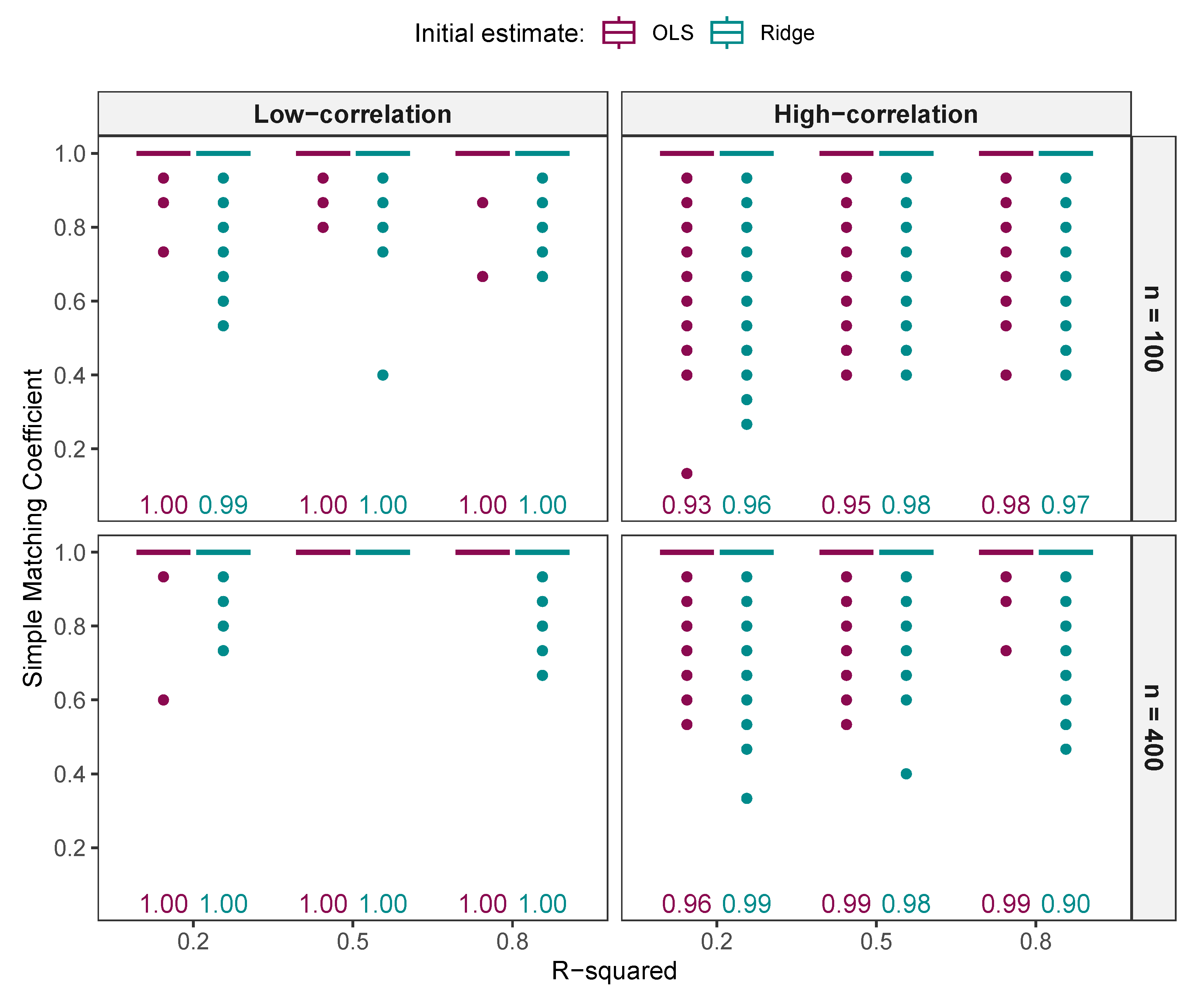
Figure 1. Boxplots comparing the SMC for variables selected by NNG and ALASSO ( γ = 1 ) using OLS and ridge initial estimates. The upper and lower panels display the results for small ( n = 100 ) and large ( n = 400 ) sample sizes, respectively, while the left and right panels show the results for the low (C2) and high (C4) correlation settings, respectively. The plots also show the proportion of 10,000 replications in which SMC = 1 across various R 2 values. For a large sample size with low correlation and R 2 values of 0.5 and 0.8, both approaches selected the same variables when OLS initial estimates were used.
Stats 08 00070 g001
Figure 2. Boxplots comparing the SMC for variables selected by NNG and ALASSO ( γ = 2 ) using OLS and ridge initial estimates. The upper and lower panels display the results for small ( n = 100 ) and large ( n = 400 ) sample sizes, respectively, while the left and right panels show the results for low (C2) and high (C4) correlations, respectively. The plots show the proportion of 10,000 replications in which SMC = 1 across various R 2 values. A high level of similarity was observed in large sample sizes with low correlation and high R 2 .
Stats 08 00070 g002
Figure 3. Comparison of average FNR, FPR, MCC, and the number of variables selected by NNG and ALASSO (with γ values of 0.5, 1, and 2) using OLS initial estimates in low-correlation settings with a large sample size ( n = 400 ). The results for NNG and ALASSO ( γ = 1 ) are almost identical, as shown by the overlapping lines. The horizontal dashed line in the bottom right panel indicates the number of true signal variables (7). Bars with a size of one standard error were added, but are not visible due to the small standard errors resulting from the large number of simulation repetitions.
Stats 08 00070 g003
Figure 4. Boxplots of Manhattan distances between regression estimates from NNG and ALASSO ( γ = 1 ) using OLS and ridge initial estimates. Results are shown for small sample sizes (upper panel) and large sample sizes (lower panel) under low correlation (left panel) and high correlation (right panel) across various R 2 values. Each plot also reports the proportion of 10,000 replications with a Manhattan distance of zero. Outlying distances are omitted.
Stats 08 00070 g004
Figure 5. Boxplots comparing Manhattan distances of regression estimates for NNG and ALASSO ( γ = 2 ) using OLS and ridge initial estimates. The plots display results for small sample sizes (upper panel) and large sample sizes (lower panel) with low correlation (left panel) and high correlation (right panel) across various R 2 values. Each plot also shows the proportion of 10,000 replications with a Manhattan distance of zero. Outlying distances are not shown.
Stats 08 00070 g005
Figure 6. Comparison of prediction accuracy assessed using the RTE metric for NNG and ALASSO with different values of γ (0.5, 1, and 2). The plots display results for small sample sizes (upper panel) and large sample sizes (lower panel), with low correlation (left panel) and high correlation (right panel) across various R 2 values. The performance results of NNG and ALASSO ( γ = 1 ) were nearly identical, as shown by the overlapping lines. OLS initial estimates were used in all approaches. Bars with a size of one standard error were added, but are not visible due to the small standard errors resulting from the large number of simulation repetitions.
Stats 08 00070 g006
Figure 7. Average FNR, FPR, MCC, and number of selected variables for NNG and ALASSO (with γ values of 0.5, 1, and 2) using ridge initial estimates in low-correlation settings with sample size n = 400 and p = 1000 covariates. The results for ALASSO ( γ = 1 ) and ALASSO ( γ = 2 ) are nearly identical, as indicated by overlapping lines. The horizontal dashed line (bottom right panel) indicates the number of true signal variables (7). Bars with a size of one standard error were added, but are not visible due to the small standard errors.
Stats 08 00070 g007
Table 1. Summary of the simulation design following the ADEMP structure.
ComponentDescription
Aims and
objectives
Aim: To investigate and compare the performance of NNG and ALASSO in multivariable linear regression with respect to variable selection and prediction accuracy.
Objectives:
  • To assess the effect of the sign of the initial estimates on model selection in NNG and ALASSO
  • To evaluate the similarity between NNG and ALASSO ( γ = 0.5 , 1 , 2 ) in terms of variable selection, corresponding regression estimates, and prediction accuracy.
Data-generating
 mechanism
 (Section 2.2)
  • Training dataset
    -
    X N p ( 0 , Σ ) , where p { 15 , 1000 } and Σ R p × p . The element Σ i j is the correlation between covariates x i and x j .
    -
    y = X β + ε , where ε N ( 0 , σ 2 I n ) .
    -
    Values of β :
    *
    For p = 15 : [ 1.5 , 0 , 1 , 0 , 1 , 0 , 0.5 , 0 , 0.5 , 0 , 0.5 , 0 , 0.5 , 0 , 0 ]
    *
    For p = 1000 : same as above, with an additional 985 zeros (noise variables)
  • Correlation structure (C)
    -
    C2: Toeplitz correlation structure with Σ i j = 0 . 3 | i j | (low correlation).
    -
    C4: Empirical correlation structure based on body fat data [30], with high correlation among 13 variables and the remaining variables uncorrelated.
  • R 2 and training sample size (n)
    -
    R 2 { 0.20 , 0.50 , 0.80 }
    -
    n { 100 , 400 }
  • Number of simulation scenarios per setting
    -
    Low-dimensional setting: 1 ( β ) × 2 ( C ) × 3 ( R 2 ) × 2 ( n ) = 12 scenarios
    -
    High-dimensional setting: 1 ( β ) × 1 ( C ) × 3 ( R 2 ) × 2 ( n ) = 6 scenarios
  • Simulation runs (N)
    -
    N = 10 , 000 for low-dimensional settings
    -
    N = 1000 for high-dimensional settings
  • Test dataset for assessing predictive accuracy
    -
    The test data were independently generated using the same design as the training dataset, with a test sample size of n test = 100 , 000 .
Target of
analysis
  • Regression coefficients
  • Selection status of each covariate
  • Prediction errors on new data
Methods
(Section 2.4)
  • Variable selection methods: NNG and ALASSO
  • Initial estimates: OLS and ridge
  • Tuning: 10-fold CV minimizing MSE
Performance
measures
(Section 2.3)
  • Regression estimates (NNG and ALASSO): compared using MD
  • Variable selection: assessed using SMC, FPR, FNR, and MCC
  • Prediction accuracy: evaluated using RTE
Table 2. Matches and mismatches between NNG and ALASSO in a hypothetical variable selection example. Rows and columns indicate the selection status under each method (1 = selected, 0 = excluded). Each cell reports the number of variables in each selection combination.
ALASSO: 0ALASSO:1
NNG: 0a = 1b = 1
NNG: 1c = 1d = 2
Table 3. Comparison of NNG and ALASSO ( γ = 0.5 , 1 , 2 ) weights based on hypothetical standardized initial estimates, ordered from weakest to strongest effect.
β ^ init ALASSO ( γ = 0.5 )ALASSO ( γ = 1 )ALASSO ( γ = 2 )NNG
0.0110.00100.0010,000.00100.00
0.054.4720.00400.0020.00
1.50.820.670.440.67
40.500.250.060.25
Table 4. Comparison of NNG and ALASSO estimates under an orthonormal design. The γ values for ALASSO are shown in brackets. Dashed lines denote zero coefficients. It can be seen that NNG and ALASSO ( γ = 1 ) produce identical estimates.
Variable β ^ init NNGALASSO (0.5)ALASSO (1)ALASSO (2)ALASSO (10)
x 1 0.06
x 2 0.12
x 3 0.20
x 4 0.300.13
x 5 0.410.160.250.16
x 6 0.910.790.800.790.780.64
x 7 1.201.121.111.121.141.19
x 8 1.521.451.431.451.471.51
x 9 2.011.961.941.961.982.00
x 10 4.013.983.963.984.014.01
Table 5. Effect of sign changes in initial estimates on NNG and ALASSO ( γ = 1 ) model selection and coefficient estimates. The columns correspond to models using: (1) the original OLS initial estimates β ^ init ; (2) β ^ init with the sign of x 1 reversed; and (3) all signs reversed ( β ^ init ). ‘–’ denotes a zero coefficient.
(1) β ^ init (Original)(2) β ^ init with x 1 Reversed(3) β ^ init (All Reversed)
Variable β ^ init NNGALASSO β ^ init NNGALASSO β ^ init NNGALASSO
x 1 1.511.511.51−1.511.51−1.511.51
x 2 0.020.020.26−0.02
x 3 1.031.021.021.031.081.02−1.031.02
x 4 −0.01−0.010.010.37
x 5 1.000.990.991.000.970.99−1.000.99
x 6 0.020.02−0.02
x 7 0.510.500.500.510.520.50−0.510.50
x 8 −0.05−0.050.050.21
x 9 0.550.530.530.550.530.53−0.550.53
x 10 0.000.00−0.00
x 11 0.390.390.390.390.410.39−0.390.39
x 12 0.040.04−0.04
x 13 −0.47−0.45−0.45−0.47−0.45−0.450.47−0.45
x 14 −0.04−0.040.04
x 15 0.040.04−0.04
Table 6. Comparison of selected variables and regression estimates between NNG and ALASSO ( γ = 0.5 , 1 , 2 ) using ridge initial estimates. MD denotes the Manhattan distance between the estimated coefficients of NNG and each ALASSO variant.
NNGALASSO ( γ = 0.5 )ALASSO ( γ = 1 )ALASSO ( γ = 2 )
Not SelectedSelectedNot SelectedSelectedNot SelectedSelected
Not Selected22,0727022,142022,1348
Selected10131014129112
MD24.170.8511.39
Disclaimer/Publisher’s Note: The statements, opinions and data contained in all publications are solely those of the individual author(s) and contributor(s) and not of MDPI and/or the editor(s). MDPI and/or the editor(s) disclaim responsibility for any injury to people or property resulting from any ideas, methods, instructions or products referred to in the content.