Review

Archimedean Copulas: A Useful Approach in Biomedical Data—A Review with an Application in Pediatrics

by
Giulia Risca
1,
Stefania Galimberti
1,2,
Paola Rebora
1,2,
Alessandro Cattoni
3,
Maria Grazia Valsecchi
1,2 and
Giulia Capitoli
1,2,*
1
Bicocca Bioinformatics Biostatistics and Bioimaging Centre-B4, School of Medicine and Surgery, University of Milano-Bicocca, 20900 Monza, Italy
2
Biostatistics and Clinical Epidemiology, Fondazione IRCCS San Gerardo dei Tintori, 20900 Monza, Italy
3
Pediatrics, Fondazione IRCCS San Gerardo dei Tintori, 20900 Monza, Italy
*
Author to whom correspondence should be addressed.
Stats 2025, 8(3), 69; https://doi.org/10.3390/stats8030069 (registering DOI)
Submission received: 27 May 2025 / Revised: 24 July 2025 / Accepted: 26 July 2025 / Published: 1 August 2025
(This article belongs to the Section Statistical Methods)

Abstract

Many applications in health research involve the analysis of multivariate distributions of random variables. In this paper, we review the basic theory of copulas to illustrate their advantages in deriving a joint distribution from given marginal distributions, with a specific focus on bivariate cases. Particular attention is given to the Archimedean family of copulas, which includes widely used functions such as Clayton and Gumbel–Hougaard, characterized by a single association parameter and a relatively simple structure. This work differs from previous reviews by providing a focused overview of applied studies in biomedical research that have employed Archimedean copulas, due to their flexibility in modeling a wide range of dependence structures. Their ease of use and ability to accommodate rotated forms make them suitable for various biomedical applications, including those involving survival data. We briefly present the most commonly used methods for estimation and model selection of copula’s functions, with the purpose of introducing these tools within the broader framework. Several recent examples in the health literature, and an original example of a pediatric study, demonstrate the applicability of Archimedean copulas and suggest that this approach, although still not widely adopted, can be useful in many biomedical research settings.

1. Introduction

Any joint distribution function has a copula representation as established by Sklar in 1959 [1]. This underlines the importance of copula functions and research about and with copulas. Sklar proved that multivariate distributions can be treated as univariate marginal distributions, one for each variable, and then coupled by copula to define the dependence structure. Consequently, the most relevant advantage of copulas is that they allow us to separately model the marginal distributions and their association. In practice, they act as a bridge between the marginal distributions of the random variables of interest and the joint distribution. Hougaard in 1987 was the first to suggest a two-stage estimation procedure that consists of the estimation of the joint margins and the use of these to obtain the association parameter [2]. This approach was further developed by Shih and Louis [3]. Adopting copula functions in multivariate studies can, thus, be a profitable strategy to simplify estimation of joint distributions. In addition, the dependence in copulas is generally nonlinear. Thanks to this feature, it is easily possible to extend models beyond linear assumptions to address more general cases and more complex contexts [4]. Over the past two decades, some reviews on copula functions were drafted, especially from a theoretical perspective and in fields such as time-series analysis and economics [5,6,7]. They have also found broad application in biomedical research, especially in the validation of surrogate endpoints [8] and in survival analyses involving time-to-event models with time-dependent censoring [9]. However, given their favorable properties, they could be applied in many other clinical contexts. With this review, we aim to highlight their simplicity and flexibility in order to promote their use in clinical research. To this end, after introducing some basic theoretical concepts, with a particular focus on the Archimedean copulas, we will present a series of clinical examples that illustrate their practical application in the bivariate case. However, with this review, we aim to underscore their potential in applied medical contexts for studying the association between variables. In this field, their use remains relatively limited and not well established.
In this review, we will first define the copula functions and their fundamental properties. Among the many available families, we will focus on a particular class known as Archimedean copulas [10]. Archimedean copulas are popular in applications because they have a simple structure, can model different types of dependence, and have other useful properties, such as associativity. This property makes it easy to extend them to higher dimensions [11]. However, for simplicity, we will illustrate the bivariate case. Moreover, by simple transformations, copulas in this class can be rotated to cover a wider range of variable associations. Consequently, selection methods for copula functions can be employed to identify the most suitable copula. We will briefly introduce the most common approaches available to select for the best bivariate copula function, like the Akaike Information Criterion (AIC), Bayesian Information Criterion (BIC) [12], and Minimum Distance Method [13]. Our overview of copula usage will be complemented by application examples from clinical research. In particular, we will refer to the setting of surrogate endpoint validation in clinical trials where a relevant step is to assess the strength of association between two outcomes, i.e., the true clinical endpoint and the corresponding candidate surrogate marker. In this context, we will show how (semi-) competing risks, dependent censoring, and truncation can be handled by using different copula based models without the constraints of linearity and censoring. Some others relevant fields of application will be explored like omics data, toxicity estimation and rare diseases. It is worth noting, however, that the examples discussed are limited to bivariate Archimedean copulas and their rotated forms, given their simplicity of use and practical flexibility in modeling dependence structures.
Briefly, the paper is organized as follows. In Section 2, we present copula theory, focusing on the aspects that are useful to apply the Archimedean class with more flexibility in the context of health data. In Section 3, we illustrate how to estimate the association parameter by different approaches like for example the Inference Function for Margins (IFM), the Maximum Likelihood Estimation (MLE), or the Method of Moments. In Section 4, we illustrate how to select the optimal copula among the various possible functions. In Section 5, we introduce some tests on the goodness of fit of a chosen copula. In Section 6, we show a series of possible copula’s applications in biomedical research and in Section 7, we present an application of the proposed copula-based methods to a previously published pediatric clinical dataset [14]. In Section 8, we summarize our conclusions.

2. Copula

In what follows, we focus on the copula bivariate case; however, all remarks can be generalized in the n-dimensional space [7].
  • We consider I = [ 0 , 1 ] , the unit segment, and I 2 = [ 0 , 1 ] × [ 0 , 1 ] ; then, we define the copula functions below.
Definition 1. 
Function C : I 2 I is called a copula if it is 2-monotone, and, for any u, v [ 0 , 1 ] it is C ( 0 , v ) = C ( u , 0 ) = 0 and C ( 1 , v ) = v , C ( u , 1 ) = u .
  • From the definition, it follows that for any copula C ( u , v ) partial derivatives C u and C v exist for almost all u, v I . Let 2 C u v and 2 C v s . u exist and be continuous on I 2 ; then, copula density is designed as
    c ( u , v ) = 2 C u v = 2 C v s . u .
  • From the definition, if u = F X ( x ) and v = G Y ( y ) , where u and v have uniform distributions on I, then any copula C ( u , v ) = C ( F X ( x ) , G Y ( y ) ) is a valid bivariate distribution function. Hence, the joint probability density function of X and Y can be represented as
    f ( x , y ) = 2 C u v d F X d x d G Y d y ,
    where d F X d x and d G Y d y are marginal densities of X and Y.
  • The more relevant property is that every joint distribution function is a copula, as demonstrated by Sklar’s theorem below [15].
Theorem 1. 
Let X and Y be random variables with distribution functions F X and G Y , respectively, and joint distribution function H. Then, there exists a copula C such that, for all x, y,
H ( x , y ) = C ( F X ( x ) ,   G Y ( y ) ) .
If F and G are continuous, then C is unique.
  • The importance of this theorem is that every valid bivariate (or multivariate) distribution can be represented as a copula of its marginals, thus separating the marginal from the dependence modeling. Consequently, in order to define a model for a bivariate distribution with given marginals, we only need to find the proper copula which, according to Sklar’s theorem, exist and is often unique. In practical terms, they allow to model the joint behavior of variables by separately specifying their marginal distributions F X ( x ) , G Y ( y ) and their dependence structure by the Copula function (this is not trivial, as we will see later). Given the previous theorem and the observation that X and Y are independent if and only if H ( x , y ) = F X ( x ) G Y ( y ) for all x,y, we can derive the following:
Theorem 2. 
Let X and Y be continuous random variables. Then, X and Y are independent if and only if C ( F X ( x ) , G Y ( y ) ) = F X ( x ) G Y ( y ) [15].

2.1. Archimedean Copula

The Archimedean copulas are widely used because their construction is relatively easy and they include several functions with good properties for applications in health data.
The following definitions are essential to identify a subclass of copulas with transformations which support additivity, while for a more extended description we refer to Genest and Maka [16].
Let Φ be a class of functions ϕ : [ 0 , 1 ] [ 0 , ] that have two continuous derivatives on ( 0 , 1 ) and satisfy ϕ ( 1 ) = 0 , ϕ ( t ) < 0 , ϕ ( t ) > 0 , for all 0 < t < 1 . These requisites allow ϕ to have an inverse ϕ 1 that also has first and second derivatives. In addition, we define the pseudo-inverse of ϕ as follows:
ϕ [ 1 ] ( t ) = ϕ 1 ( min ( t , ϕ ( 0 ) ) )
So, ϕ [ 1 ] ( t ) = ϕ 1 ( t ) if 0 t ϕ ( 0 ) and ϕ [ 1 ] ( t ) = 0 if t > ϕ ( 0 ) . Moreover, if ϕ ( t ) when t 0 , then the pseudo-inverse function is equivalent to the inverse function. The pseudo-inverse is helpful to extend the inverse transformation to the functions of limited range. Based on this, the central theorem of this subsection follows (for the proof, see [15]).
Theorem 3. 
Let ϕ : [ 0 , 1 ] [ 0 , ] be a continuous, strictly decreasing function such that ϕ ( 1 ) = 0 . Then, the function
C ( u , v ) = ϕ [ 1 ] ( ϕ ( u ) + ϕ ( v ) )
is a copula if and only if ϕ is convex.
  • If C ( u , v ) fulfils these conditions, it is called an Archimedean copula and the function ϕ ( t ) is its additive generator. Hereafter, we state two theorems regarding the main algebraic properties of Archimedean copula.
Theorem 4. 
Let C be an Archimedean copula with generator ϕ. Then:
1. 
C is symmetric; i.e., C ( u , v ) = C ( v , u ) for all u,v I ;
2. 
C is associative, i.e., C ( C ( u , v ) , w ) = C ( u , C ( v , w ) ) for all u,v,w I ;
3. 
If c > 0 is any constant, then c ϕ is also a generator of C.
  • A useful condition to assess if an arbitrary copula is an Archimedean copula is the following:
Theorem 5. 
Let C be an associative copula such that δ C ( u ) < u for all u I , where δ C ( u ) = C ( u , u ) is the diagonal projection of a copula. Then, C is Archimedean.
  • Finally, given that the second derivative ϕ ( t ) exists, we define the density of an Archimedean copula through its generator and its derivatives as
    c ( u , v ) = 2 C u v = ϕ ( C ( u , v ) ) ϕ ( u ) ϕ ( v ) ( ϕ ( C ( u , v ) ) ) 3 .
  • At the moment, we are interested in three one-parameter families from the Archimedean class, namely the Clayton copula, the Gumbel–Hougaard copula, and the Frank copula.
The Clayton copula [17] is generated by ϕ ( t ) = 1 θ ( t θ 1 ) and it takes the form
C θ ( u , v ) = ( u θ + v θ 1 ) 1 θ , if u θ + v θ 1 0 0 , otherwise θ [ 1 , ) { 0 }
where θ is the dependence parameter that indicates the strength of association between u and v. As θ approaches zero, u and v become independent, whereas they are positively associated for θ > 0 .
The Gumbel–Hougaard copula [18], generated by ϕ ( t ) = ( ln t ) θ , has the following form:
C θ ( u , v ) = exp { [ ( ln u ) θ + ( ln v ) θ ] 1 θ } , θ 1
Small values of θ provide a positive strong association and independence is achieved when θ 1 .
Frank’s copula was proposed in the context of financial studies, but it is also useful in other contexts. The generator is ϕ ( t ) = ln ( e x p ( θ t ) 1 ) / ( e x p ( θ ) 1 ) and it leads to
C θ ( u , v ) = 1 θ ln 1 + [ e x p ( θ u ) 1 ] [ e x p ( θ v ) 1 ] e x p ( θ ) 1
where θ ( , ) { 0 } . As θ approaches zero, u and v become independent. Moreover, it has a positive association when θ > 0 and a negative association when θ < 0 , as shown in Figure 1.

2.2. Measures of Concordance

The strength of the association in the copula model is expressed by the copula parameter θ . Nevertheless, interpreting this parameter may be difficult and cannot help in the direct comparison of different models. Kendall’s concordance-coefficient τ was proposed as an alternative indicator for measuring association. Its advantage is that this coefficient is independent from the marginal distributions of the two random variables X and Y and it depends only on the copula function C θ . In particular, Kendall’s τ is defined as the probability of concordance minus the probability of discordance of two independent realizations of ( X , Y ) each with bivariate distribution function H ( x , y ) [15]. So, if we consider ( X 1 , Y 1 ) and ( X 2 , Y 2 ) , they are concordant if ( X 1 X 2 ) > 0 and ( Y 1 Y 2 ) > 0 or if ( X 1 X 2 ) < 0 and ( Y 1 Y 2 ) < 0 . Conversely, they are discordant if ( X 1 X 2 ) > 0 and ( Y 1 Y 2 ) < 0 or if ( X 1 X 2 ) < 0 and ( Y 1 Y 2 ) > 0 . Thus, Kendall’s τ is defined by
τ = P [ ( X 1 X 2 ) ( Y 1 Y 2 ) > 0 ] P [ ( X 1 X 2 ) ( Y 1 Y 2 ) < 0 ]
It assumes values in [ 1 , 1 ] , and it is zero when X i and Y i are independent. In addition, Kendall’s τ can be obtained from θ by the following transformation [15]:
τ = 4 0 1 0 1 C θ ( u , v ) C θ ( d u , d v ) 1
Another measure of the association is Spearman’s rank-correlation coefficient ρ [15]. It is defined to be proportional to the probability of concordance minus the probability of discordance of three independent realizations of ( X , Y ) , with common joint distribution function H ( x , y ) . For example, if the pairs considered are ( X 1 , Y 1 ) and ( X 2 , Y 3 ) , where the first pair of random variables has H ( x , y ) as bivariate joint distribution function and the second one has independent components Spearman’s rank-correlation coefficient is defined as
ρ = 3 ( P [ ( X 1 X 2 ) ( Y 1 Y 3 ) > 0 ] P [ ( X 1 X 2 ) ( Y 1 Y 3 ) < 0 ] )
Also, it holds the following relationship with θ :
ρ = 12 0 1 0 1 C θ ( u , v ) d u d v 3 , ρ [ 1 , 1 ]
In the bivariate case of the Archimedean family, Kendall’s τ correlation coefficient is
τ = 1 + 4 0 1 ϕ ( t ) ϕ ( t ) d t .
The relationship between θ and Kendall’s τ for Clayton’s model is τ = θ / ( θ + 2 ) , while it is τ = ( θ 1 ) / θ for Gumbel–Hougaard’s model. These two families do not have a closed form for Spearman’s ρ , whereas, for the Frank copula, both Kendall’s τ and Spearman’s ρ form can be written by means of the Debye function D k ( x ) = ( k / x k ) 0 x t k / ( e x p ( t ) 1 ) d t , where Kendall’s τ becomes
τ θ = 1 4 θ [ 1 D 1 ( θ ) ]
and Spearman’s ρ is
ρ θ = 1 12 θ [ D 1 ( θ ) D 2 ( θ ) ]
These expressions are analytically intractable and typically require a numerical approximation, making the use of the Frank copula less practical.
Not all copulas cover the full spectrum of the possible types of association (positive or negative). If they do so, they are called comprehensive. The Frank copula is comprehensive, whereas the Clayton and Gumbel–Hougaard copula are not, as they only capture positive dependence between u and v. Nevertheless, we recall the opportunity to exploit the rotated copulas to overcome this limitation (see Section 2.3).

2.3. Rotated Copulas

A relevant feature not yet widely used in applications concerns the ability to rotate the copula functions. Rotations expand the types of associations that a copula approach can address. However, the dependence between variables can vary between 1 and 1 and not all previously defined copulas are able to capture a negative dependency between u and v (e.g., Clayton and Hougaard copulas), thus limiting applications in many contexts. According to Cech [20], different types of rotations are available, which give a copula that satisfies definition 1. The most used ones are:
  • 90 rotated (reflected) copula: C + ( u , v ) = u C ( 1 u , v ) , where
    c + ( u , v ) = c ( 1 u , v ) is the density of the copula.
  • 180 rotated copula: C ( u , v ) = u + v 1 + C ( 1 u , 1 v ) ,
    where c ( u , v ) = c ( 1 u , 1 v ) is the density of the copula.
    This particular rotation defines the survival copula that we will discuss in Section 2.3.1.
  • 270 rotated (reflected) copula: C + ( u , v ) = u C ( u , 1 v ) , where c + ( u , v ) = c ( u , 1 v ) is the density of the copula.
With these transformations, many different forms of data dependence can be properly fitted with the family of Archimedean copulas, and not only. Of note, Kendall’s τ and Spearman’s ρ of a copula and of its associated rotated copula are not different. We only point out that the reflections ( u , v ) ( u , 1 v ) and ( u , v ) ( 1 u , v ) reverse the sign of both Kendall’s τ and Spearman’s ρ , highlighting how such transformations affect the direction of dependence [21].

2.3.1. Survival Copula

A special case of the rotated copulas are the survival copulas. They are of interest to state the Sklar’s theorem for survival marginal functions. In contexts where the random variables X and Y denote the lifetime (or time to failure) of an individual or a device, we might want to model the survival functions S X ( x ) = 1 F X ( x ) = P ( X x ) and S Y ( y ) = 1 G Y ( y ) = P ( Y y ) and their joint survival function S ( x , y ) = P ( X x , Y y ) . As consequence, we enunciate via survival copula the relationship between the joint survival distribution and the survival marginal functions in the following way:
S ( x , y ) = P ( X x , Y y ) = P ( ( X x ) c ( Y y ) c ) = = 1 P ( ( X x ) ( Y y ) ) = = 1 ( P ( X x ) + P ( Y y ) P ( ( X x ) ( Y y ) ) ) = = 1 F X ( x ) G Y ( y ) + H ( x , y ) = = S X ( x ) + S Y ( y ) 1 + C ( F X ( x ) , G Y ( y ) ) = = S X ( x ) + S Y ( y ) 1 + C ( 1 S X ( x ) , 1 S Y ( y ) )
Now, if we define C ¯ ( u , v ) as a copula with marginals u and v as follows
C ¯ ( u , v ) = u + v s . 1 + C ( 1 u , 1 v ) ,
then we obtain that S ( x , y ) = C ¯ ( S X ( x ) , S Y ( y ) ) , equivalently to Sklar’s theorem. C ¯ ( u , v ) is called survival copula, a 180 rotation of the standard copula and satisfies all copula properties as defined in Section 2. However, if the copula function arises from Archimedean family, the corresponding survival copula is not necessarily an Archimedean copula. In fact, the generator of the survival copula might not satisfy the convexity condition required by the Theorem 3, even if the original generator does.
  • From the definition, we note that
    C ¯ ( u , v ) u = 1 C ( 1 u , 1 v ) u ,
    and equivalently with respect to v.

2.3.2. Examples on Rotated Archimedean Copulas: Clayton and Hougaard

We focus here on the survival copula, so according to (6), we apply the 180 rotation to the Clayton (1) and the Gumbel–Hougaard (2) copula.
  • The Clayton survival copula has the following form for θ > 0 :
    C ¯ θ ( u , v ) = u + v 1 + ( ( 1 u ) θ + ( 1 v ) θ 1 ) 1 θ ,
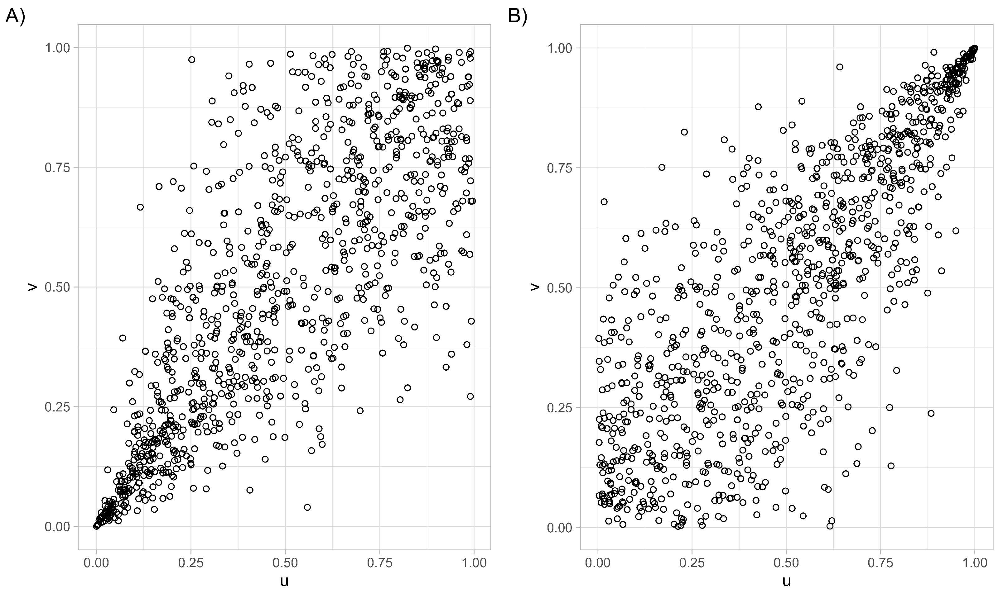
    Figure 2 illustrates how the survival Clayton copula emphasizes strong upper-tail dependence, in contrast to the lower-tail dependence captured by the standard Clayton copula. In the latter, a strong association is expected near the point (0, 0), whereas in the survival copula, strong dependence is expected as ( u , v ) approaches (1, 1).
Figure 2. Simulated data by the r package copula [19] from the Clayton copula (A) and the Clayton survival copula (B). The parameter of association was equal to 3 in both.
Stats 08 00069 g002
The Hougaard survival copula has the following form:
C ¯ θ ( u , v ) = u + v 1 + exp { [ ( ln ( 1 u ) ) θ + ( ln ( 1 v ) ) θ ] 1 θ } , θ 1
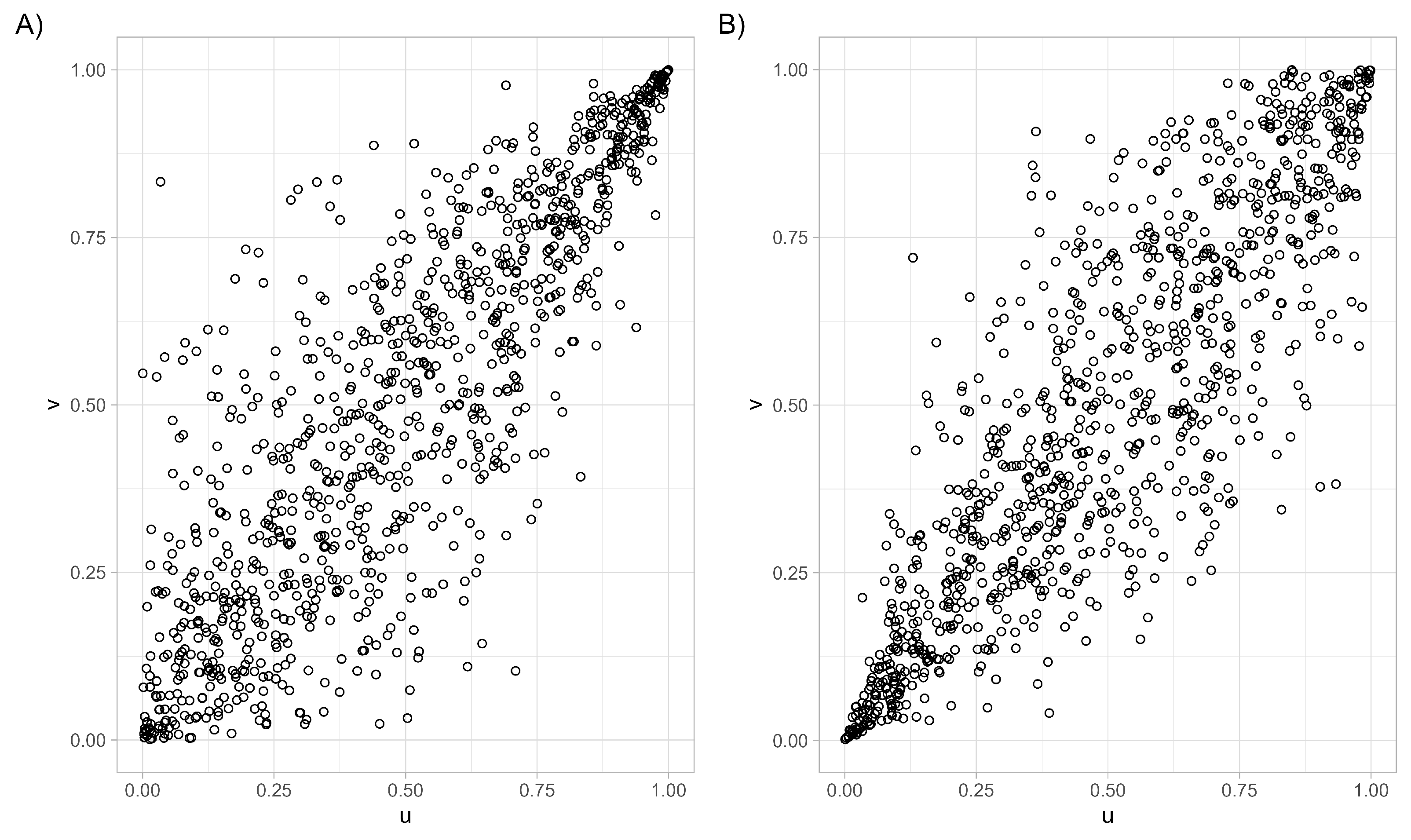
The Hougaard copula works opposite to the Clayton, and hence, we expect a strong association when ( u , v ) is near to ( 1 , 1 ) for the standard formulation and near to ( 0 , 0 ) for the survival copula.
Figure 2 and Figure 3 show the dissimilar behaviour of these copula’s families and thus, the reason why they are often chosen to investigate the different relationships between variables.
The central issue is the marginals’ choice to use the cumulative distribution function F X ( x ) or survival function S X ( x ) to give the direction of the implementation [22]. For example, imagining to use the survival marginal functions with the Clayton copula, we observe a stronger association near ( 0 , 0 ) or where event time are largest. If we instead apply the survival marginal functions to the Clayton survival copula, we observe a stronger association near ( 1 , 1 ) , corresponding to smaller event times. As a result, it is important to choose both the copula and the dependence direction carefully, based on the characteristics of the data and the objectives of the analysis.
A relevant peculiarity of Frank’s copula is that it is the only one of the Archimedean family that has the same form for the copula and the survival copula, i.e., C θ ( u , v ) = C ¯ θ ( u , v ) . Equivalently, it is radially symmetric, see Nelsen [15] for an accurate definition and a proof of the equivalence. Despite this advantageous property, the Frank copula is often not chosen because the concordance parameters cannot be easily measured. For this reason, the Plackett copula, a non-Archimedean copula, is sometimes suggested as an alternative and is briefly described in the following section.

2.4. Plackett Copula

The Plackett family construction [23,24] derives from a generalization of the odds ratio to the bivariate distributions with continuous margins and it is assumed as constant. As a consequence, the copula function is defined as follows:
C θ ( u , v ) = 1 + ( u + v ) ( θ 1 ) K θ ( u , v ) 2 ( θ 1 ) if θ 1 u v otherwise
where
K θ ( u , v ) = [ 1 + ( θ 1 ) ( u + v ) ] 2 + 4 θ ( 1 θ ) u v
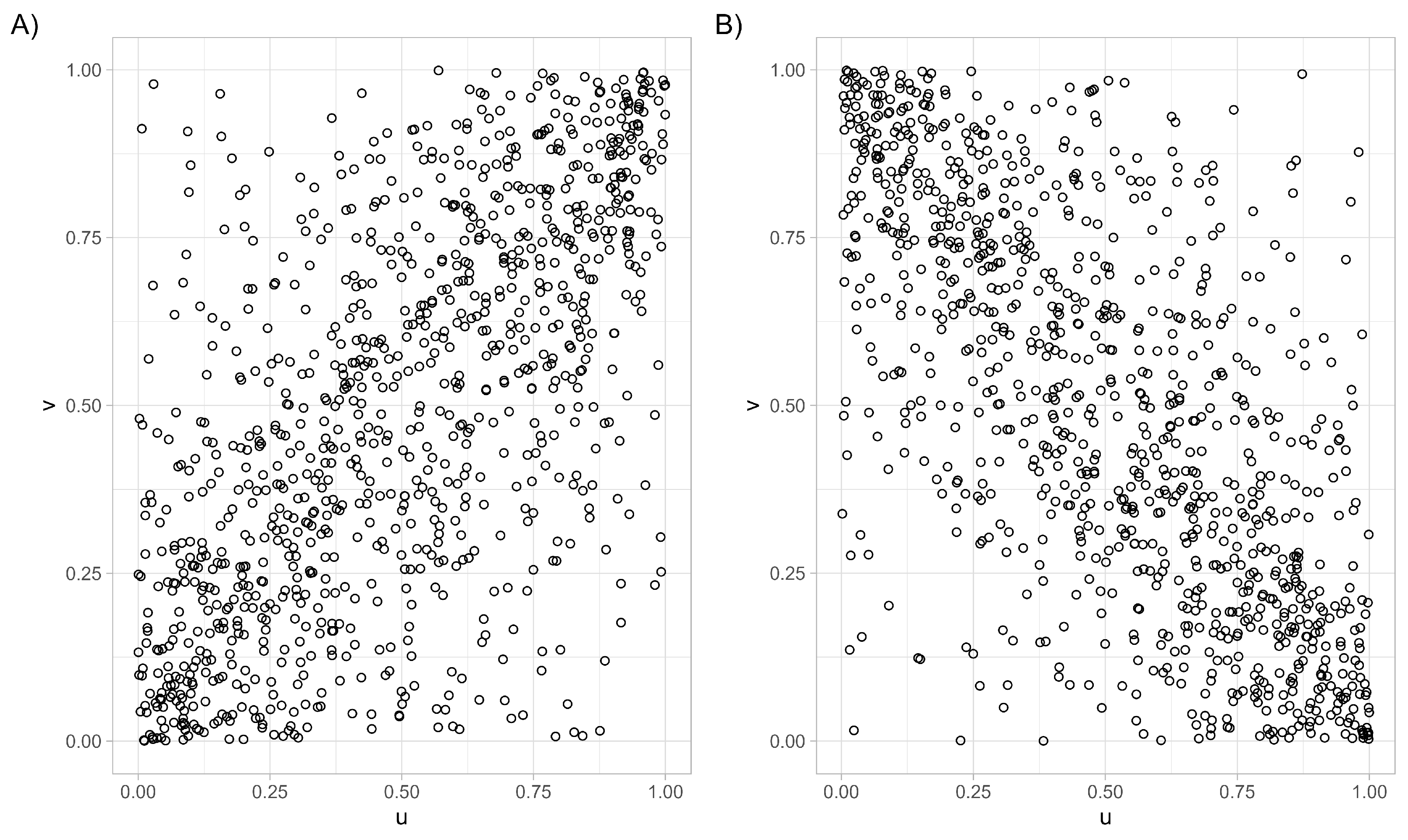
and θ [ 0 , ] . The association is negative or positive according to whether θ < 1 or θ > 1 , respectively. This behavior is illustrated in Figure 4. A value of θ = 1 corresponds to independence. As a closed form expression for Kendall’s τ cannot be derived, Spearman’s ρ = ( θ + 1 ) / ( θ 1 ) 2 θ / ( θ 1 ) 2 log θ is used in applications.

3. Estimation Methods

When a parametric form is assumed for the marginal distributions, two approaches can be used for estimating copula parameters: the Inference Function for Margins (IFM) [25] and the Maximum Likelihood Estimation (MLE). The first method relies on the fundamental property of copulas, allowing for a two-step estimation process: first the marginals, then the dependence structure. Instead, the second approach estimates all parameters in one step, thus requiring a high number of derivations. The latter is preferable when the marginal distributions are given and a large sample is available, due to its asymptotic optimality property. Nevertheless, similar to IFM, an alternative to MLE is the Maximum Pseudo-Likelihood Estimation method (MPLE), which estimates the dependence parameter in the second step, after considering in the first step the estimation of the marginals instead of their values. When no assumptions on the parametric form of marginal distributions [26] are made, the approach used is the Canonical Maximum Likelihood (CML) method that estimates the association parameter as in the IFM.
However, the most used and fast estimation method is the Method of Moments, where the measures of concordance represent the moments. Based on the relationship function between the copula parameter and the moments, as for example (4) or (5), the sample moments are estimated via the theoretical definition of moments and the association parameters are subsequently obtained by plugging in the estimated sample moments in the functions (4) or (5). This approach is reasonable when the copula family has one-parameter, as in the Archimedean class, while it is less so when there are more parameters and it is not trivial to interpret the moments. The association parameter of some Archimedean functions can also be estimated via a Minimum Distance (MD) approach. To do so, it is necessary to define the empirical Kendall’s measure:
K n ( t ) = i = 1 n 1 ( T i t ) n + 1
where T i = j = 1 n 1 { X j X i & Y j Y i } / ( n + 1 ) , i = 1 , 2 , n are the pseudo-observations. Also, we define the theoretical Kendall function K θ ( t ) = P ( C θ ( u , v ) t ) corresponding to the true model. Afterwards, we estimate θ by the θ ^ M D that minimizes the distance
d K = i = 1 n ( K n ( t ) K θ ( t ) ) 2 1 / 2 .
All the methods we briefly outlined here are explained with more details in Shemyakin and Kniazev [27].
Additionally, we illustrate a nonparametric method to estimate the dependence parameter specifically for Archimedean copulas [28]. Starting from the usual estimate of Kendall’s correlation coefficient of (3):
τ ^ = n 2 i < j S i g n [ ( X i X j ) ( Y i Y j ) ]
and considering the identity
τ = 1 + 4 0 1 ϕ ( t ) ϕ ( t ) d t ,
where ϕ ( t ) is a function of θ ; we can estimate θ ^ solving the following in θ :
τ ^ = 1 + 4 0 1 ϕ ( t ) ϕ ( t ) d t .
In particular, for the Clayton and Gumbel–Hougaard models we can directly refer to the relationship τ ^ = θ / ( θ + 2 ) and τ ^ = ( θ 1 ) / θ , respectively.
Finally, it is worth mentioning that the estimation procedure can also be performed according to a Bayesian approach. This is particularly appealing when a noninformative prior is assumed for the distribution of the association parameter, π ( θ ) , and the posterior distribution is estimated as usual as π ( θ | u , v ) π ( θ ) L ( θ | u , v ) . We refer to [29] to see how this approach is used once the proper copula function is chosen.

4. How to Select the Bivariate Copula Functions

In applications, which copula can best fit our set of data is a very relevant question. Given what is shown, it is important to choose the copula function for the model of study based on a prior exploration that suggests the better copula for our data. In this process, we can apply one of the estimation methods such as MLE, MPLE, Method of Moments [30], and Bayesian estimation, but we can also use a hybrid approach, i.e., a combination of previous methods. In particular, one can use the MPLE to estimate the association parameters of two different copula families and then compare them with the empirical concordance by the Method of Moments to select the model which appears more appropriate. In addition, it is possible to combine the Minimum Distance with MPLE or MLE method. However, the approaches more commonly adopted to select a copula family are the Akaike Information Criterion, AIC [31], or the Bayesian Information Criterion, BIC [12].
In general, the information criteria measure the relative loss of information when the copula C is fitted to the data in place of the true underling copula. It depends on the likelihood function L ( x ; θ ) , and focuses on its maximization.
In particular, in the AIC method, the model with the lower value of A I C = 2 ln L ( x ; θ ) + 2 k , where k is the dimension of θ , is considered the better copula, as AIC is minimized for the best trade-off between goodness of fit and model complexity. So, a higher dimension penalizes the copula model. Instead, in the BIC method the penalization depends also an the sample size n, as B I C = 2 ln L ( x ; θ ) + k ln ( n ) . Another meaningful method is the Minimum Distance Method [13], which is vastly applied to identify the most appropriate bivariate Archimedean copula [32]. It consists of the comparison between the empirical and the theoretical estimation of the one-dimensional distribution function of the Archimedean copula K ( t ) , respectively, K n ( t ) and K ϕ ( t ) . The first one is determined through the pseudo-observation T i , thanks to which we calculate the K n ( t ) , as defined in (7). Instead, the second one is K ϕ ( t ) = t ϕ ( t ) / ϕ ( t ) . Then, the Minimum Distance Method is applied to measure the closeness between K n ( t ) and K ϕ ( t ) and select the best copula to fit the observed data. Other metrics are available to base the selection choice, such as for example D M = ( K ϕ ( t ) K n ( t ) ) 2 d K n ( t ) , used in [33] to select the best copula. A graphic analysis, contrasting K n with K ϕ for example via QQ-plot [34], may also be a useful way to compare the the empirical and theoretical quantiles, with the limitations of any graphical check. The closer they lie along the diagonal, the better the copula fits the data.

5. The Goodness of Fit

The goodness of fit is a test that is helpful to evaluate the quality of a given copula family in representing the data distribution. To this purpose, several tests are available [26] according to different needs. The null hypothesis is that a copula (with parameter θ ) exists and expresses the joint distribution, equivalently H 0 : C C 0 , where C 0 = { C θ : θ O } is a copula family. We primarily focus on the comparison between the empirical copula function C n ( u , v ) = 1 n i = 1 n I ( U i u , V i v ) and C θ n , an estimator of C under the H 0 . Moreover, θ n is a θ estimation based on the pseudo-observations T i , seen before. The most commonly used distance measures used to compare the empirical and the parametric copula are (for simplicity, in what follows, we refer to u and v with the vector u ):
  • Kolmogorov–Smirnov distance: n max n | C n C θ n |
  • Cramer–von Mises distance: [ 0 , 1 ] 2 ( C n ( u ) C θ n ( u ) ) 2 d C n ( u )
  • Anderson and Darling distance: max n | C n C θ n | C θ n ( 1 C θ n )
  • Average of Anderson and Darling distance: [ 0 , 1 ] 2 | C n C θ n | C θ n ( 1 C θ n ) d C n ( u )
It can be shown that the Kolmogorov–Smirnov and Cramer–von Mises distances differ from Anderson and Darling distances for their higher sensitivity to deviations in the center of the distribution rather than in the tails.
Through the sample simulations with the estimated copula’s parameters θ n , we can construct the distribution of the distance measures under the null hypothesis of accurate fit and based on this, we can approximate the p-values. Genest and Remillard [35] proved that if the C 0 and the θ n are regular in some sense, they converge and the test is consistent.
In a similar way, one can test the goodness of a given copula by a test based on Kendall’s transformation [28,36,37]. In this case, the test statistic compares the empirical Kendall’s distribution mentioned in (7) and a parametric estimation of K θ , the distribution of C ( F ( X ) , G ( Y ) ) when C = C θ C 0 . Also, it is necessary to estimate θ by the relationship (4) to obtain the estimator K θ n of K θ . Then, the hypothesis H 0 : K K 0 = { K θ : θ O } can be tested by one of the distance measure mentioned before between the empirical Kendall and K θ n . Genest et al. in [36], using as the statistic a rank-based version of Kolmogorov–Smirnov and Cramer–von Mises distances, determined that if the distance value is large the H 0 is to be rejected. Nevertheless, under regularity conditions on C 0 , K 0 and θ n , the convergence is demonstrated. In addition, we note that the current hypothesis H 0 corresponds to the previous H 0 only in Archimedean case. Also, Rosenblatt’s transformation [38] may be used to construct a goodness-of-fit test as Genest et al. have explored in [26].
These comparisons can also be tested graphically through the QQ-plots, or quantile-quantile plots, or a graphical measure of the distance between a copula/Kendall’s τ and some “true” distribution.

6. Significant Applications of Copulas

Copula functions are applied in many fields [39]; initially, mostly in economics and finance, but more recently also in biology, epidemiology, and clinical research. Here, they are helpful to model the joint distribution of variables of interest with great adaptability, making the approach more general than standard ones. Furthermore, they offer some advantages in the models’ construction, as we will see below. We will specifically focus on Archimedean copulas given that they offer analytical tractability, ease of construction in the bivariate case and of simulation, and interpretable measures of dependence, which make them appealing for biomedical data analysis. However, we also acknowledge the importance of other types of copulas for describing not only bivariate, but also more complex dependence structures. In particular, copulas like the Gaussian, Vine, and Plackett copulas are especially valuable in higher-dimensional or elliptical dependence settings. Moreover, copulas such as the Farlie–Gumbel–Morgenstern family and other variants can be useful in specific contexts due to their interpretability and simplicity [40,41]. However, for simplicity and ease of interpretation, especially for a clinical audience, we focused on example with Archimedean copulas.

6.1. Nonnormality and Nonlinear Dependence Assumption

In the bivariate probit model, the use of copula functions has the aim to introduce the nonnormality assumption, as shown in an application in health economy [42]. The standard bivariate probit model is widely implemented to estimate the effect of an endogenous binary regressor, such as an experimental versus a control treatment, on a binary outcome variable, such as response. The copula approach can maintain normal marginals for the two errors of the bivariate probit model, but releases the full bivariate normality condition through the copula joint distribution function.
Copulas allow to relax the bivariate normality assumption in the so called selection models [43], i.e., they lead to a model with a nonlinear association between the selection variable, which expresses the consent to undergo a diagnostic test and the response to the test itself. Two different equations for the variables selection and response are defined and then joint by copulas. In particular, the authors favored a copula family oriented toward a rotation of Archimedean copulas to describe a negative association [43], since those who undergo diagnostic testing tend to be negative. This example shows how rotated copulas can be applied in epidemiology.
For prediction models in clinical research, the copula approach might be more appropriate than the correlation models [44]. Since copula functions merge both the linear and nonlinear dependence, they offer a lot of families to model data association when handling directly the marginal distributions for different types of outcomes.

6.2. Survival Data and Validation of Surrogate Endpoints

Copula functions are extensively used to study the association between endpoints in clinical trials [45]. In particular, they are suitable to develop models to validate endpoints as surrogate of a true endpoint. For example, various models were developed to study whether a candidate endpoint measured early after treatment might be a valid surrogate for a well-recognized clinical endpoint, such as survival, evaluated later during follow up, for assessing treatment effect. In this regard, the most common approach is the meta-analytic copula method by Burzykowski et al. [8,46]. Copulas easily apply to different couples of endpoints, mixing binary, ordinal, longitudinal, and time to event survival, allowing for different choices of marginals. The model matches the marginal functions of the two variables (surrogate and true endpoint) by copula and then by the Maximum Likelihood function estimates the association parameter across different clinical trials. There are many extension that cover a wide range of cases, such as categorical [47] and left or right censored or truncated candidate surrogate endpoints. In addition, for bivariate time-to-event data, Petti et al. [48] developed a copula regression model to estimate the relationship between outcomes where a mix of uncensored, left-, right-, and interval-censored data occurred. The motivation of the significant use of copulas is attributable to the possibility of treating marginals separately. Indeed, it is easier to construct the marginal distributions and subsequently to estimate the association parameter of copula than to analyze directly the joint distribution.
Another application of the copula model concerns the validation of a time-to-event surrogate endpoint that collects information from the true clinical outcome to construct the candidate surrogate endpoint, for example the progression-free survival as surrogate for overall survival [49]. The authors also explored the impact of a small number of clinical trials with a small sample size of patients.

6.3. Competing Risks

Another setting where copula models have found an application is that of competing risks. In this context, there is a failure process with various potential causes of failure and the time to the first event among those determining the failure is the quantity of interest. Escalera et al. [50] first, and later Adatorwovor et al. [51] extended through copulas the standard statistical methods for competing risks, addressing the case when causes of failure cannot be assumed to be independent. In this situation, the copula functions allow to jointly consider the cause-specific survival functions. In addition, Michimae et al. [52] derived a Bayesian estimator for copula-based dependent competing risks models under left-truncated data, with strong performances. Also, models to measure the association between endpoints in the presence of semi-competing risks have been addressed with copulas. In this setting, the occurrence of a terminal event prevents the observation of a nonterminal event, and, given that they belong to the same individual, it is reasonable to investigate the relation between the two times to event [53]. Hence, the structure of association between the two outcomes follows a copula function [54]. In addition, due to the possibility of a nonconstant association over time this model is implemented by Archimedean copulas and not only with normal copula.
A particular situation related to competing risks was studied by Choi et al. [55], who investigated the penetrance of a second event of interest when successive competing risks occur. In other words, a subject is exposed to the risk of a first event of interest (or death), and immediately after, they are exposed to a second event of interest or death. They proposed to model via copula the dependence between the successive events, as for example the occurrence of a second cancer.

6.4. Omics Data

Another attractive extension concerns the use of the Cox regression model. This was applied to identify genes influencing the survival in a cohort of patients with lung cancer [56]. While standard survival methods assume independence between survival and censoring times, a copula approach is able to formalize a dependence structure between the survival and censoring marginal functions. This flexibility of copula functions allows to relax the independent censoring assumption when this is not appropriate for the data context.

6.5. Toxicity

In oncology and in many other medical areas, therapy consists of the combination of multiple drugs. In finding the dose level of each drug composing the treatment, toxicity related to the drug’s combination must be assessed. Thanks to copula functions, it is possible to develop a model for the joint toxicity probabilities having the marginals of the probability of toxicity for each single drug [57].
Another interesting application in the context of clinical trial is to consider a model for evaluating jointly the treatment effect on efficacy and toxicity. These two outcomes are both relevant and may be correlated. Tao et al. [58] proposed an Archimedean copula model to jointly estimate efficacy and toxicity. The choice of this type of approach is guided by the good properties of simplicity, flexibility, and adaptability to handle both continuous outcomes and mixed outcomes.

6.6. Rare Diseases

A potentially appealing field of application that we are currently exploring is the use of copulas in data simulations in the setting of rare diseases. The idea is to first study the association between either treatment or biomarker and the outcome in a small sample collected on a disease where, by definition, the number of patients that can be enrolled is very limited due to the rarity. Subsequently, a simulation protocol based on a copula approach able to mimic the association previously explored can be applied to generate an in silico (larger) trial [59].

7. Application in a Pediatric Study

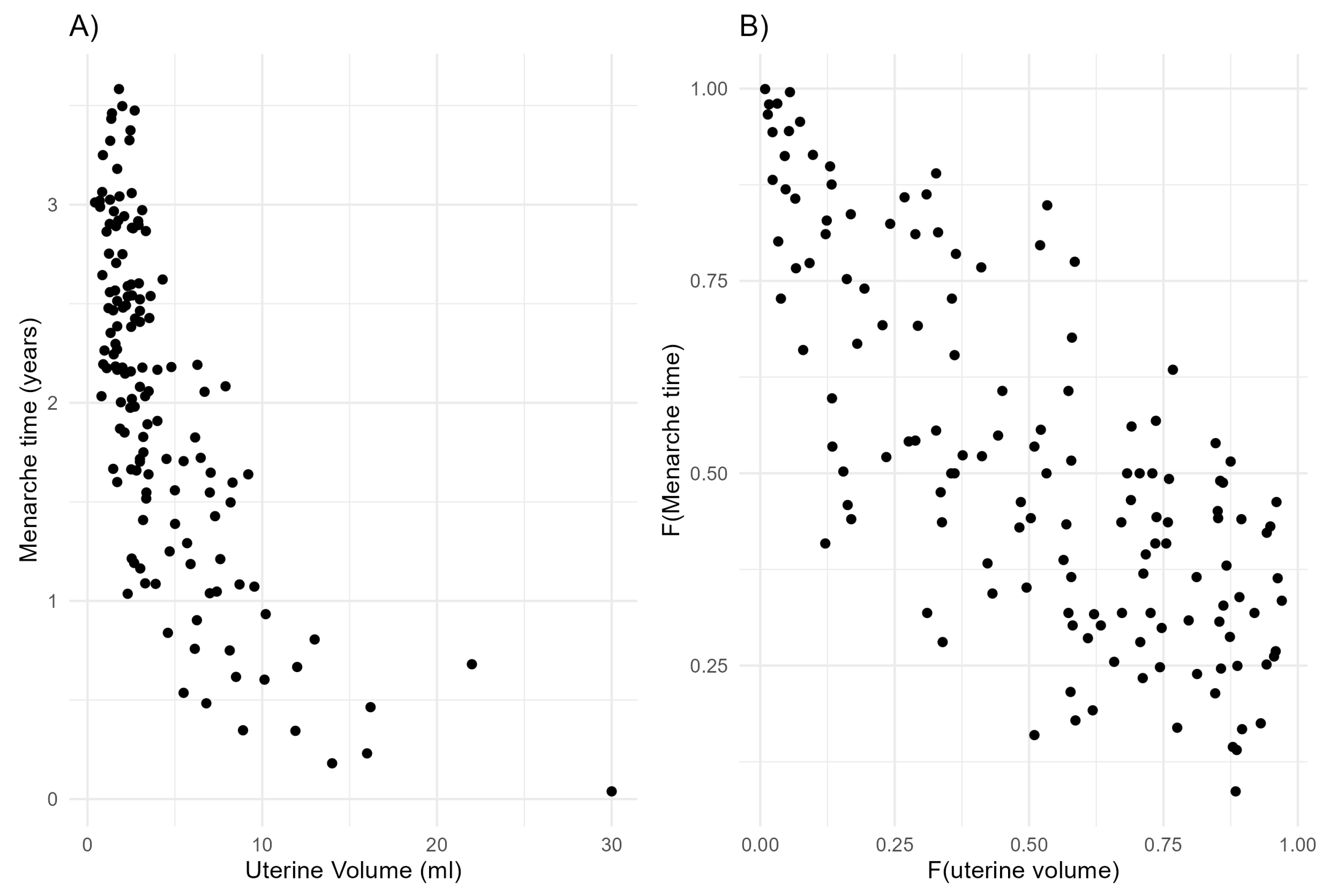
In this section, we apply the methods discussed in the previous sections to a data from a clinical study on pubertal development in girls with early signs of puberty [14]. The study included 94 girls referred for evaluation of early pubertal signs, who underwent pelvic ultrasound and clinical assessments, and were followed over time to record the occurrence and timing of menarche. At baseline, ultrasound parameters such as uterine and ovarian volume were recorded, along with hormonal profiles and clinical data. The main aim of the original analysis was to investigate whether uterine volume could serve as a predictor of pubertal progression, particularly in anticipating the time to menarche. The association between the two variables is illustrated in Figure 5A, which clearly shows their nonlinear relationship. Previous analyses in the original study highlighted a predictive role of uterine volume with respect to pubertal timing. Here, we further explore this nonlinear relationship using copula-based models, to evaluate whether the dependence structure between the two variables is consistent with our expectations and whether it can be quantified through copula parameters. Among the patients included, we focus on those with available and reliable measurements of both uterine volume and follow-up data on menarcheal age. Using rotated Gumbel copula ( 90 rotation to capture negative dependence; see Figure 5B), we measure the strength of the association between the cumulative distribution functions (CDFs) of uterine volume and time to menarche. The CDF of uterine volume is estimated by a gamma distribution, whereas time to menarche’s CDF by a gaussian distribution. The association between the CDFs estimated by the copula parameter is 2.12 ( 95 % CI = 2.01–2.23), corresponding to a Kendall τ of approximately 0.53 . It suggests a moderately strong negative association: larger uterine volumes are associated with shorter times to menarche. This finding confirms the results of the original publication and provides additional support for the association through a more flexible dependence modeling framework. The consistency across methods reinforces the value of uterine volume as an early, noninvasive marker of pubertal progression.

8. Conclusions

We briefly reviewed the copula theory to show the significant properties of this approach and the advantages for application on health data. We posed our attention on the Archimedean family given that its functions are easy to handle and meet many needs in the fields of application we presented. The possibility to rotate a copula from this family is an important extension that can capture the relationship between variables of various type. Rotations are still rarely used, but we recommend them to increase the goodness of fit in case of positive associations or to fit negative associations. This is more direct than the method used by Burzykowski et al. in chapter 7 of [60], where they model a negative association only after data transformation (i.e., the negative logarithm of one of the two variable of interest). We also recommend to pay attention to the opportunity to choose between modeling the cumulative distribution function or the survival distribution function to give the direction of the implementation.
We illustrated a number of possible applications for copulas in medical research through various recently published papers. In addition, we showcased the use of copula modeling in a pediatric clinical setting, revealing a nonlinear association between uterine volume and the age at menarche. The flexibility of Archimedean copulas, particularly when allowing for rotation—enabled us to capture this relationship more accurately than standard linear models, by better reflecting the underlying nature of the association.
Although copulas have been present in the literature for quite some time, their application in clinical research remains relatively limited. Nonetheless, our work highlights their potential as a useful tool for tackling complex clinical and statistical challenges, particularly in the presence of asymmetric distributions. They are able to describe a nonlinear dependence by allowing a flexible arbitrary choice of the marginal distributions. They are also helpful to describe skewed outcomes and to overcome the assumption of dependent censoring. Even though many applications exist, like those in time-series, clustering, and in machine learning in economics and finance settings [39], unfortunately, copulas do not play a central role in health science yet. In conclusion, copulas are a valid way to construct and assess complex associations between outcomes, thus providing a valid opportunity for innovation and methodological research in the context of biomedical data.

Author Contributions

Conceptualization, and formal analysis G.R. and G.C.; writing—original draft preparation, G.R. and G.C.; writing—review and editing, M.G.V. and P.R.; data curation, A.C.; visualization, G.R.; supervision, S.G.; project administration, M.G.V.; funding acquisition, S.G. and P.R. All authors have read and agreed to the published version of the manuscript.

Funding

G.R. and P.R were funded by the European Union—Next Generation EU—NRRP M6C2—Investment 2.1 Enhancement and strengthening of biomedical research in the NHS project code PNRR-MAD-2022-12376033 (CUP: H43C22001270006), title “Evidence-based models for high impact chronic disease prevention and risk of progression management in outpatient community services and community hospitals: towards eHealth integrating stratification on individual history with predictive models of disease progression, using machine learning and artificial intelligence on administrative and clinical databases”, PI Antonio Giampiero Russo. S.G. and M.G.V. participated in the manuscript preparation during their personal involvement in the Italian Ministry of University MUR Dipartimenti di Eccellenza 2023–2027 (l. 232/2016, art. 1, commi 314–337). S.G. and M.G.V. were partially supported by the grant PRIN 2022SYXEH. This work has received funding from the European Union—NextGenerationEU through the Italian Ministry of University and Research under the PNRR-M4C2-I1.3 Project PE_00000019 “HEAL ITALIA” to G.C. The views and opinions expressed are those of the authors only and do not necessarily reflect those of the European Union or the European Commission. Neither the European Union nor the European Commission can be held responsible for them.

Institutional Review Board Statement

Not applicable.

Informed Consent Statement

Not applicable.

Data Availability Statement

Not applicable.

Conflicts of Interest

The authors declare no conflicts of interest.

Abbreviations

The following abbreviations are used in this manuscript:
IFMInference Function for Margins
MLEMaximum Likelihood Estimation
MPLEMaximum Pseudo-Likelihood method
CMLCanonical Maximum Likelihood
MDMinimum Distance
AICAkaike Information Criterion
BICBayesian Information Criterion
CDFCumulative Distribution Function

References

  1. Sklar, A. Fonctions de répartition à n dimensions et leurs marges. Publ. Inst. Statist. Univ. Paris 1959, 8, 229–231. [Google Scholar]
  2. Hougaard, P. Modelling Multivariate Survival. Scand. J. Stat. 1987, 14, 291–304. [Google Scholar]
  3. Shih, J.H.; Louis, T.A. Inferences on the Association Parameter in Copula Models for Bivariate Survival Data. Int. Biom. Soc. 1995, 51, 1384–1399. [Google Scholar] [CrossRef]
  4. Clementi, F.; Gianmoena, L. Chapter 9—Odeling the Joint Distribution of Income and Consumption in Italy: A Copula-Based Approach With k-Generalized Margins. In Introduction to Agent-Based Economics; Gallegati, M., Palestrini, A., Russo, A., Eds.; Academic Press: Cambridge, MA, USA, 2017; pp. 191–228. [Google Scholar] [CrossRef]
  5. Fan, Y.; Patton, A.J. Copulas in Econometrics. Annu. Rev. Econ. 2014, 6, 179–200. [Google Scholar] [CrossRef]
  6. Patton, A.J. A review of copula models for economic time series. J. Multivar. Anal. 2012, 110, 4–18. [Google Scholar] [CrossRef]
  7. Kolev, N.; Anjos, U.D.; Mendes, B.V.D.M. Copulas: A review and recent developments. Stoch. Model. 2006, 22, 617–660. [Google Scholar] [CrossRef]
  8. Burzykowski, T.; Molenberghs, G.; Buyse, M.; Geys, H.; Renard, D. Validation of Surrogate End Points in Multiple Randomized Clinical Trials with Failure Time End Points. J. R. Stat. Soc. Ser. C (Appl. Stat.) 2001, 50, 405–422. [Google Scholar] [CrossRef]
  9. Crommen, G.; Deresa, N.W.; D’Haen, M.; Ding, J.; Willems, I.; Keilegom, I.V. Recent advances in copula-based methods for dependent censoring. SORT 2025, 49, 3–42. [Google Scholar] [CrossRef]
  10. Nadarajah, S.; Afuecheta, E.; Chan, S. A compendium of Copulas. Statistica 2017, 4, 279–328. [Google Scholar] [CrossRef]
  11. Genest, C.; Nešlehová, J.; Ziegel, J. Inference in multivariate Archimedean copula models. Test 2011, 20, 223–256. [Google Scholar] [CrossRef]
  12. Schwarz, G. Estimating the dimension of a model. Ann. Stat. 1978, 6, 461–464. [Google Scholar] [CrossRef]
  13. Wolfowitz, J. The Minimum Distance Method. Ann. Math. Stat. 1957, 28, 75–88. [Google Scholar] [CrossRef]
  14. Cattoni, A.; Russo, G.; Capitoli, G.; Rodari, G.; Nicolosi, M.L.; Molinari, S.; Tondelli, D.; Pelliccia, C.; Radaelli, S.; Arosio, A.M.L.; et al. Pelvic ultrasound and pubertal attainment in girls with sexual precocity: The pivotal role of uterine volume in predicting the timing of menarche. Front. Endocrinol. 2024, 15, 1417281. [Google Scholar] [CrossRef]
  15. Nelsen, R.B. An Introduction to Copulas, 2nd ed.; Springer Series in Statistics; Springer: Berlin/Heidelberg, Germany, 2006. [Google Scholar]
  16. Genest, C.; Mackay, J. The Joy of Copulas: Bivariate Distributions with Uniform Marginals. Am. Stat. 1986, 40, 280–283. [Google Scholar] [CrossRef]
  17. Clayton, D.G. A Model for Association in Bivariate Life Tables and Its Application in Epidemiological Studies of Familial Tendency in Chronic Disease Incidence. Oxf. J. 1978, 65, 141–151. [Google Scholar] [CrossRef]
  18. Hougaard, P. A Class of Multivariate Failure Time Distributions. Oxf. J. 1986, 73, 671–678. [Google Scholar] [CrossRef]
  19. Yan, J. Enjoy the Joy of Copulas: With a Package Copula; Technical Report; University of Connecticut: Storrs, CT, USA, 2007. [Google Scholar]
  20. Cech, C. Copula-Based Top-Down Approaches in Financial Risk Aggregation; Working Paper Series; University of Applied Sciences of BFI Vienna: Wien, Austria, 2006; Volume 32. [Google Scholar]
  21. Georges, P.; Lamy, A.G.; Nicolas, E.; Quibel, G.; Roncalli, T. Multivariate survival modelling: A unified approach with copulas. SSRN Electron. J. 2001. [Google Scholar] [CrossRef]
  22. Renfro, L.A.; Shang, H.; Sargent, D.J. Impact of copula directional specification on multi-trial evaluation of surrogate end points. J. Biopharm. Stat. 2015, 25, 857–877. [Google Scholar] [CrossRef]
  23. Plackett, R.L.; Placmett, R.L. A Class of Bivariate Distributions. J. Am. Stat. Assoc. 1965, 60, 516–522. [Google Scholar] [CrossRef]
  24. Tibaldi, F.; Molenberghs, G.; Burzykowski, T.; Geys, H. Pseudo-likelihood estimation for a marginal multivariate survival model. Stat. Med. 2004, 23, 947–963. [Google Scholar] [CrossRef]
  25. Joe, H. Asymptotic efficiency of the two-stage estimation method for copula-based models. J. Multivar. Anal. 2005, 94, 401–419. [Google Scholar] [CrossRef]
  26. Genest, C.; Rémillard, B.; Beaudoin, D. Goodness-of-fit tests for copulas: A review and a power study. Insur. Math. Econ. 2009, 44, 199–213. [Google Scholar] [CrossRef]
  27. Shemyakin, A.; Kniazev, A. Introduction to Bayesian Estimation and Copula Models of Dependence, 1st ed.; John Wiley & Sons, Incorporated: Hoboken, NJ, USA, 2017; pp. 195–232. [Google Scholar]
  28. Genest, C.; Rivest, L.P. Statistical Inference Procedures for Bivariate Archimedean Copulas. J. Am. Stat. Assoc. 1993, 88, 1034–1043. [Google Scholar] [CrossRef]
  29. Cuevas, J.R.T.; Yela, J.P.; Achcar, J.A. A method to select bivariate copula functions. Rev. Colomb. Estad. 2019, 42, 61–80. [Google Scholar]
  30. Pearson, K. Method of Moments and Method of Maximum Likelihood. Biometrika 1936, 28, 34–59. [Google Scholar] [CrossRef]
  31. Akaike, H. Likelihood of a model and information criteria. J. Econom. 1981, 16, 3–14. [Google Scholar] [CrossRef]
  32. Gülöksüz, C.T. Comparison of Some Selection Criteria for Selecting Bivariate Archimedean Copulas. Afyon Kocatepe Univ. J. Sci. Eng. 2016, 16, 250–255. [Google Scholar] [CrossRef]
  33. Frees, E.W.; Valdez, E.A. Understanding Relationships Using Copulas. N. Am. Actuar. J. 1998, 2, 1–25. [Google Scholar] [CrossRef]
  34. Fernandez, V. Copula-based measures of dependence structure in assets returns. Phys. Stat. Mech. Its Appl. 2008, 387, 3615–3628. [Google Scholar] [CrossRef]
  35. Genest, C.; Remillard, B. Validity of the parametric bootstrap for goodness-of-fit testing in semiparametric models. Ann. L’Institut Henri Poincare (B) Probab. Stat. 2008, 44, 1096–1127. [Google Scholar] [CrossRef]
  36. Genest, C.; Quessy, J.F.; Rémillard, B. Goodness-of-Fit Procedures for Copula Models Based on the Probability Integral Transformation. Scand. J. Stat. 2006, 33, 337–366. [Google Scholar] [CrossRef]
  37. Wang, W.; Wells, M.T. Model Selection and Semiparametric Inference for Bivariate Failure-Time Data. J. Am. Stat. Assoc. 2000, 95, 19. [Google Scholar] [PubMed]
  38. Rosenblatt, M. Remarks on a Multivariate Transformation. Ann. Math. Stat. 1952, 23, 470–472. [Google Scholar] [CrossRef]
  39. Größer, J.; Okhrin, O. Copulae: An overview and recent developments. Wiley Interdiscip. Rev. Comput. Stat. 2022, 14, e1557. [Google Scholar] [CrossRef]
  40. Qura, M.E.; Fayomi, A.; Kilai, M.; Almetwally, E.M. Bivariate power Lomax distribution with medical applications. PLoS ONE 2023, 18, 0282581. [Google Scholar] [CrossRef]
  41. Ahmad, H.H.; Ramadan, D.A. Copula-Based Bivariate Modified Fréchet–Exponential Distributions: Construction, Properties, and Applications. Axioms 2025, 14, 431. [Google Scholar] [CrossRef]
  42. Winkelmann, R. Copula bivariate probit models: With an application to medical expenditures. Health Econ. 2012, 21, 1444–1455. [Google Scholar] [CrossRef]
  43. McGovern, M.E.; Bärnighausen, T.; Marra, G.; Radice, R. On the assumption of bivariate normality in selection models. Epidemiology 2015, 26, 229–237. [Google Scholar] [CrossRef]
  44. Kumar, P.; Shoukri, M.M. Copula based prediction models: An application to an aortic regurgitation study. BMC Med. Res. Methodol. 2007, 7, 21. [Google Scholar] [CrossRef]
  45. Weber, E.M. Statistical Models to Capture the Association Between Progression-free and Overall Survival in Oncology Trials. Ph.D. Thesis, Lancaster University, Lancaster, UK, 2020. [Google Scholar]
  46. Burzykowski, T.; Molenberghs, G.; Buyse, M. The Evaluation of Surrogate Endpoints; Springer: Berlin/Heidelberg, Germany, 2005. [Google Scholar]
  47. Galimberti, S.; Devidas, M.; Lucenti, A.; Cazzaniga, G.; Möricke, A.; Bartram, C.R.; Mann, G.; Carroll, W.; Winick, N.; Borowitz, M.; et al. Validation of Minimal Residual Disease as Surrogate Endpoint for Event-Free Survival in Childhood Acute Lymphoblastic Leukemia. JNCI Cancer Spectr. 2018, 2, pky069. [Google Scholar] [CrossRef]
  48. Petti, D.; Eletti, A.; Marra, G.; Radice, R. Copula link-based additive models for bivariate time-to-event outcomes with general censoring scheme. Comput. Stat. Data Anal. 2022, 175, 107550. [Google Scholar] [CrossRef]
  49. Dimier, N.; Todd, S. An investigation into the two-stage meta-analytic copula modelling approach for evaluating time-to-event surrogate endpoints which comprise of one or more events of interest. Pharm. Stat. 2017, 16, 322–333. [Google Scholar] [CrossRef] [PubMed]
  50. Escarela, G.; Carrière, J.F. Fitting competing risks with an assumed copula. Stat. Methods Med. Res. 2003, 12, 333–349. [Google Scholar] [CrossRef] [PubMed]
  51. Adatorwovor, R.; Latouche, A.; Fine, J.P. A parametric approach to relaxing the independence assumption in relative survival analysis. Int. J. Biostat. 2022, 18, 577–592. [Google Scholar] [CrossRef] [PubMed]
  52. Michimae, H.; Emura, T.; Miyamoto, A.; Kishi, K. Bayesian parametric estimation based on left-truncated competing risks data under bivariate Clayton copula models. J. Appl. Stat. 2024, 51, 2690–2708. [Google Scholar] [CrossRef]
  53. Huang, C.H.; Chen, Y.H.; Wang, J.L.; Wang, M. Semiparametric copula-based analysis for treatment effects in the presence of treatment switching. Stat. Med. 2020, 39, 2936–2948. [Google Scholar] [CrossRef]
  54. Sorrell, L.; Wei, Y.; Wojtyś, M.; Rowe, P. Estimating the correlation between semi-competing risk survival endpoints. Biom. J. 2021, 64, 131–145. [Google Scholar] [CrossRef]
  55. Choi, Y.H.; Briollais, L.; Win, A.K.; Hopper, J.; Buchanan, D.; Jenkins, M.; Lakhal-Chaieb, L. Modeling of successive cancer risks in Lynch syndrome families in the presence of competing risks using copulas. Biometrics 2017, 73, 271–282. [Google Scholar] [CrossRef]
  56. Emura, T.; Chen, Y.H. Gene selection for survival data under dependent censoring: A copula-based approach. Stat. Methods Med. Res. 2016, 25, 2840–2857. [Google Scholar] [CrossRef]
  57. Yin, G.; Yuan, Y. Bayesian dose finding in oncology for drug combinations by copula regression. Appl. Statist. 2009, 58, 211–224. [Google Scholar] [CrossRef]
  58. Tao, Y.; Liu, J.; Li, Z.; Lin, J.; Lu, T.; Yan, F. Dose-finding based on bivariate efficacy-toxicity outcome using archimedean copula. PLoS ONE 2013, 8, e78805. [Google Scholar] [CrossRef]
  59. Owzar, K.; Pranab, K.S. Copulas: Concepts and novel applications. METRON-Int. J. Stat. 2003, LXI, 323–353. [Google Scholar]
  60. Alonso, A.; Bigirumurame, T.; Burzykowski, T.; Geert, M.B.; Leacky, M.; Nolen, M.; Perualila, J.; Shkedy, Z.; Elst, W.V.D. Applied Surrogate Endpoint Evaluation Methods with SAS and R; CRC Biostatistics Series; Chapman & Hall: London, UK, 2017. [Google Scholar]
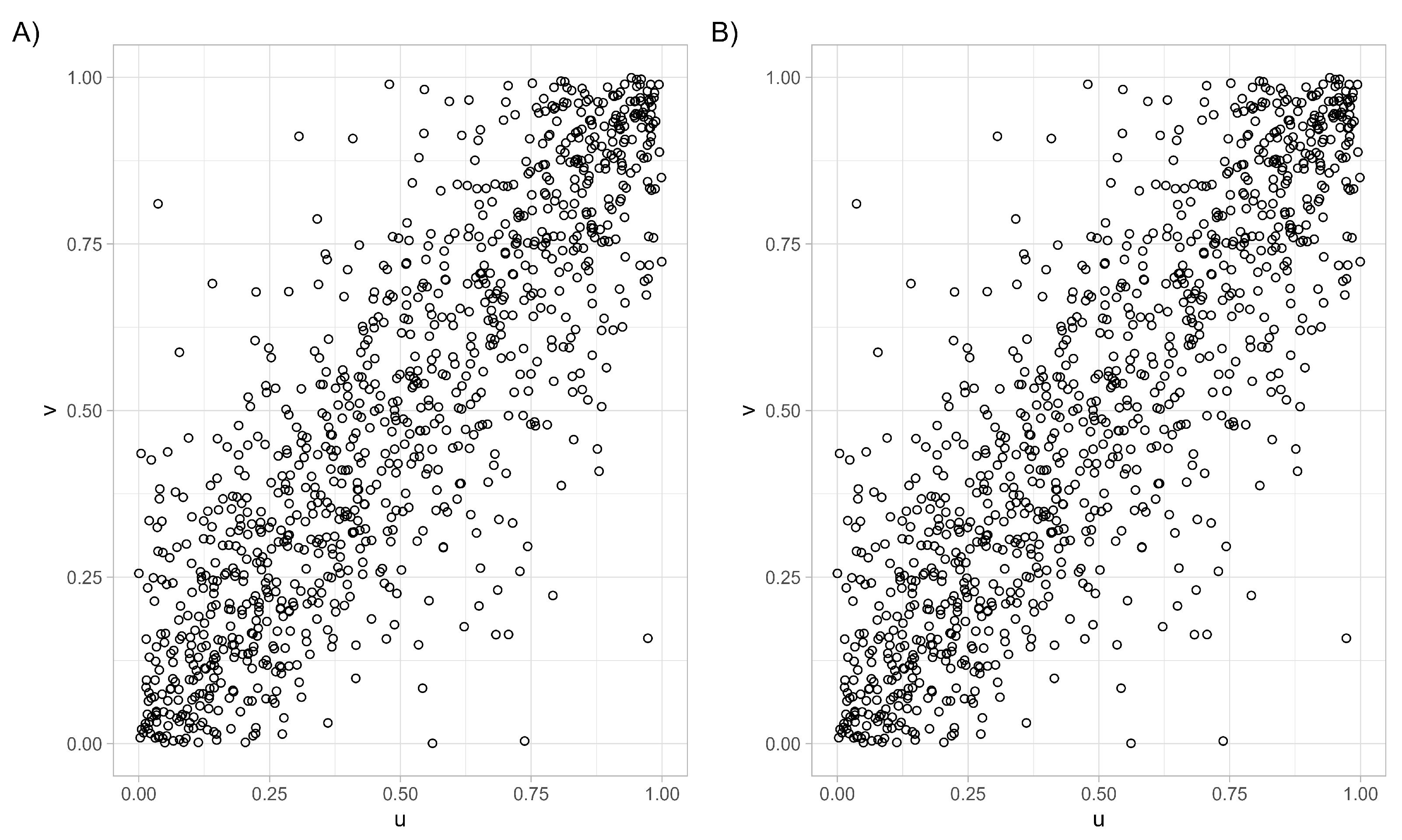
Figure 1. Simulated data by the r package copula [19] from the Frank copula function with a positive (A) or negative (B) parameter of association.
Stats 08 00069 g001
Figure 3. Simulated data by the r package copula [19] from the Gumbel–Hougaard copula (A) and the Gumbel–Hougaard survival copula (B). The parameter of association was equal to 3 in both.
Stats 08 00069 g003
Figure 4. Simulated data by the r package copula [19] from the Plackett copula function with a positive (A) or negative (B) parameter of association.
Stats 08 00069 g004
Figure 5. (A) Relationship between uterine volume and time to menarche. (B) Relationship between the corresponding cumulative distribution functions: gaussian distribution for time to menarche and gamma distribution for uterine volume.
Stats 08 00069 g005
Disclaimer/Publisher’s Note: The statements, opinions and data contained in all publications are solely those of the individual author(s) and contributor(s) and not of MDPI and/or the editor(s). MDPI and/or the editor(s) disclaim responsibility for any injury to people or property resulting from any ideas, methods, instructions or products referred to in the content.