Automated Classification of Crime Narratives Using Machine Learning and Language Models in Official Statistics

Abstract

This paper presents the implementation of a language model–based strategy for the automatic codification of crime narratives for the production of official statistics. To address the high workload and inconsistencies associated with manual coding, we developed and evaluated three models: an XGBoost classifier with bag-of-words features and word embeddings features, an LSTM network using pretrained Spanish word embeddings as a language model, and a fine-tuned BERT language model (BETO). Deep learning models outperformed the traditional baseline, with BETO achieving the highest accuracy. The new ENUSC (Encuesta Nacional Urbana de Seguridad Ciudadana) workflow integrates the selected model into an API for automated classification, incorporating a certainty threshold to distinguish between cases suitable for automation and those requiring expert review. This hybrid strategy led to a 68.4% reduction in manual review workload while preserving high-quality standards. This study represents the first documented application of deep learning for the automated classification of victimization narratives in official statistics, demonstrating its feasibility and impact in a real-world production environment. Our results demonstrate that deep learning can significantly improve the efficiency and consistency of crime statistics coding, offering a scalable solution for other national statistical offices.

1. Introduction

As part of their operations, national statistical offices (NSOs) collect information in free-text format. Examples include textual narratives about occupation, economic activity, consumption or production. To make this information useful from an applied statistical perspective, it must be coded—a task traditionally performed manually within NSOs. To ensure high-quality labeled data, trained coders read each record individually and assign the appropriate code based on a classification system.

Manual coding is time-consuming and requires the consistent application of complex criteria by multiple individuals, which is no easy task, given that classification systems are typically extensive and governed by numerous rules that are not always straightforward to learn or apply. As a result, and supported by improved access to computational tools, NSOs have begun shifting toward automatic coding using supervised learning techniques [1,2,3].

This approach relies on a previously manually labeled dataset to train an algorithm capable of learning the coding rules and applying them to new records. Although this strategy entails initial costs related to data processing and model training, once satisfactory performance is achieved, generating predictions takes only a fraction of the time required for manual coding.

Several cases of machine learning-based coding for occupation, production, and economic activity in statistical offices have been reported in the literature [4,5]; however, no documented experiences exist in the context of victimization data. This paper presents a successful case of deep learning-based coding applied to crime narratives from ENUSC (use National Urban Survey on Citizen Security for its name in english), conducted by the National Statistics Institute (INE) of Chile.

The data to be coded consist of textual narratives describing crimes reported by victims. To perform the coding, three language model–based approaches are evaluated: one using the XGBoost algorithm, another based on a deep learning model, and a third leveraging a transformer-based language model. The first approach uses XGBoost with pretrained word embeddings as the language representation, and its performance is compared to that of a traditional bag-of-words representation. The second is an LSTM model that also uses pretrained word embeddings. The third approach employs BERT, a transformer-based language model trained exclusively on Spanish text and fine-tuned for the task. The results show that the language model approaches achieve high accuracy in coding crime narratives, leading to the decision to deploy the model in production.

This study presents a novel contribution to official statistics by applying and evaluating automated methods for the classification of open-text crime narratives. Beyond demonstrating the feasibility of using deep learning in this context, the work provides a comparative analysis of different modeling strategies—including traditional machine learning and modern language models—highlighting the trade-offs in performance, computational cost, and infrastructure requirements. This perspective is especially relevant for national statistical offices (NSOs) with limited resources. Additionally, this paper proposes a threshold-based framework for selecting high-certainty predictions, offering a practical methodology to integrate automated classifiers into production workflows while maintaining quality standards.

This paper is structured as follows. First, the conceptual framework for crime coding is described. Second, several experiences in statistical offices are reviewed. Third, the results are presented, with particular emphasis on the process of putting the model into production and adapting the ENUSC workflow to incorporate the developed models. Through the deployment of an API (Application Programming Interface), a prediction service is made available to the business team, which allows for easy modification of the existing processing code to incorporate an automatic coding stage. Finally, the conclusions and discussion of the work are presented.

2. Codification Framework

ENUSC, starting from its twentieth edition, adopts a codification based on three references. These are the VICLAC-LACSI initiative, the International Classification of Crimes for Statistical Purposes [6], and the coding historically used by ENUSC in its previous editions. Based on these sources, the aim is to establish a balance between international comparability and national relevance.

The United Nations Office on Drugs and Crime (UNODC) is the primary international entity dedicated to promoting measurement standards for criminal phenomena through National Statistical Offices. In 2010, it published the Manual for Victimization Surveys as a descriptive guide to best practices being developed by NSOs in this area. In 2015, UNODC-INEGI Center of Excellence marked a new milestone with its initiative for victimization surveys in Latin America and the Caribbean, offering a methodology, model questionnaire, and standardized indicators for the region.

This methodology includes the measurement of core and non-core crimes (see

Table 1. Core and annex crimes, defined by UNODC [7].

Core Crimes	Annex Crimes
Vehicle, truck or pick-up theft	Theft of personal property from inside the vehicle
Theft of vehicle, truck or pick-up parts	Bicycle theft
Motorcycle/scooter theft	Vandalism
Domestic burglary	Cybercrimes
Robbery	Homicide
Theft (Larceny)	Kidnapping
Bank fraud	Sexual and physical harassment
Fraud/swindling	Possession of firearms
Bribery
Physical assaults
Threats
Extortion

), with the former being those recommended for inclusion as a common denominator for crime measurement across countries adopting the standard.

This set of crimes is conceptually aligned with the International Classification of Crimes for Statistical Purposes (ICCS). This standard is based on the description of criminal events in conceptual terms rather than legal definitions, which may vary from country to country. Thus, it aims to improve the comparability of victimization statistics [6].

In the case of ENUSC, the update to its codification for 2023 references the aforementioned standards, aligning its crime measurement with international recommendations. However, as also noted by these standards, they must be adapted to the national context based on the relevance of the crimes to be measured and specific national crime-naming conventions. In line with this, ENUSC takes as a reference the crimes historically measured, which, for example, include “Surprise robbery” or “lanzazo” (known in other countries as “snatch theft”), a crime not listed in LACSI and occupying an intermediate position between theft with and without violence.

Based on these considerations, the crimes included in ENUSC 2023 and 2024 are as follows: (1) vehicle, truck or pick-up theft; (2) vehicle, truck or pick-up theft; (3) vehicle vandalism; (4) domestic burglary; (5) household vandalism; (6) robbery with violence or intimidation; (7) surprise robbery; (8) theft; (9) bank fraud; (10) fraud/swindling; (11) assaults and injuries; (12) threats; (13) extortion; (14) bribery; (15) email or social media hacking; (16) malware; (17) cyberbullying; (18) identity theft/impersonation; and (19) sexual harassment.

For the update of ENUSC 2023, based on historical data, six crimes were prioritized for review, where historical issues in classification have been identified. These crimes are vehicle vandalism, burglary with forced entry, household vandalism, bank fraud, fraud/swindling, and assaults and injuries.

Despite this selection of crimes, the workload for review remains significant, which necessitates distributing the manual review among various business analysts. In order to reduce the workload and the variability of criteria when coding, the decision was made to explore the use of automatic coding technologies, an approach that offers the potential to mitigate both issues.

3. Related Work

Due to the high cost of manual coding, national statistical offices have moved toward automated methods, which can be broadly classified into two categories: rule- or dictionary-based automation, and automation through machine learning. Within the latter, a distinction can be made between traditional machine learning approaches and those based on large language models (LLMs).

3.1. Rule-Based Codification

In the United States, companies can self-report their industry codes; however, these reports often do not align with the actual business activities. The work by [1] focuses on identifying and correcting misclassified codes, while also assigning codes to entities that have not reported any information [8]. Studies such as Chaisricharoen et al. [8] propose ontology-based systems to detect and reduce redundancies across different industry classification schemes.

The ACTR system, developed by Istat in Canada during the 1990s, uses Automatic Text Coding for classification purposes. The process begins with standardization steps such as the removal of stop words, synonym grouping, and suffix stripping. After standardization, the system compares the input with reference dictionaries to assign codes. If an exact match is found, the process is completed; otherwise, an algorithm searches for partial matches [9]. Thompson et al. [10] introduced a classification system for NAICS codes, where the process starts by generating dictionaries for each code, built using the most relevant words and n-grams associated with each industrial activity and occupation.

These dictionaries may point to multiple codes, which leads to the use of a logistic regression model to determine the most likely code. The sum of the percentages associated with each code in the lookup dictionary serves as a reference, with the code receiving the highest total being assigned as the correct one [10].

In the case of INE Chile, the Household Budget Survey uses a strategy similar to those previously mentioned to code household consumption. By searching for text strings within expenditure descriptions, a code is assigned according to the rules of the CCIF system. While this strategy successfully codes a significant portion of the records, a non-negligible fraction still requires labeling by expert coders.

3.2. Machine Learning Approach

Rule-based systems are common and serve as a baseline for coding free-text data; however, there is a growing trend toward the use of new technologies aimed at improving efficiency and reducing the amount of manual work involved in the task.

No specific experiences were found addressing published crime codification problems; however, several national statistical offices have explored and implemented machine learning approaches for similar tasks. Takahashi et al. [11] examined the automatic coding of industry and occupation in Japan using a Support Vector Machine (SVM)-based system. This system assigns each record up to three codes based on the highest certainty scores, facilitating subsequent manual verification. Based on the certainty scores of the two most likely codes, the system assigns one of three certainty levels (high, medium, or low) to the top prediction. The features used include words identified as parts of speech that can be morphologically analyzed, and rule-based classifications are incorporated when available. Their findings show that achieving 85% accuracy corresponds to 67% coverage, while increasing accuracy to 91% reduces coverage to 50%, highlighting the trade-off between accuracy and automation rate.

Numerous national statistical offices and public institutions have begun integrating machine learning techniques for the automatic coding of open-text responses in their statistical production processes. These efforts, originally focused on domains such as occupation and economic activity, have evolved toward the use of more advanced models, including Transformer-based architectures. For instance, Chile’s National Institute of Statistics (INE) has applied Support Vector Machines (SVMs) for the automatic classification of occupations and economic activities in the National Employment Survey, significantly reducing manual workload [12].

Oehlert et al. [1] employed Random Forest models due to the limited availability of data and the presence of outliers in the classification information and its features. For evaluation, they used a baseline that assumed all self-reported codes were correct and imputed the most common valid code in sectors with missing information. The Random Forest model applied to the non-informative subset achieved an accuracy of 65.7%, significantly outperforming the baseline accuracy of 16.8%.

Advances in machine learning have had a significant impact on the coding of occupations and economic activities, offering more efficient and accurate methods compared to traditional rule-based approaches. The National Institute of Statistics of Chile is aligned with this trend and, since 2019, has used Support Vector Machines (SVMs) to code occupation and economic activity data in the National Employment Survey [12,13]. The categorical cross-entropy loss is widely used in classification tasks to measure the discrepancy between the true class labels and the predicted probabilities. It penalizes incorrect predictions more when the model is confident but wrong:

$$\mathcal{L}=-\sum _{i=1}^N{y}_{i}log\left({\widehat{y}}_i\right)$$

(1)

where $\mathcal{L}$ is the total loss, N is the number of classes, $y_i$ is the true label (1 if the class is correct, 0 otherwise), and ${\widehat{y}}_i$ is the predicted probability for class i.

Language Model-Based Codification

Although deep learning is a subset of machine learning, it offers several advantageous features that enhance overall performance. A key feature is its ability to represent text densely within a vector space.

One of the early applications of deep learning for NAICS classification was reported by Wood et al. [3], who analyzed data sourced from the EverString database, comprising 18 million companies. Among the prominent features in the dataset, descriptions emerged as particularly significant for ranking purposes. Additionally, company websites provided additional information including descriptive paragraphs and links to third-party descriptions and Wikipedia articles. These texts underwent a representation phase through a weighted combination of term frequency-inverse document frequency (tf-idf) on key terms and n-gram sequences ranging from 1 to 4. The classification model employed a deep learning architecture consisting of a fully connected four-layer perceptron with a hyperbolic tangent (tanh) activation function and a final layer with a SoftMax activation for classification. This system achieved an overall accuracy of 47.9%.

Turrell et al. [14] focused on constructing statistical measures for labor market demand, leveraging data from job advertisements posted online by firms and recruitment agencies on the <Reed.co.uk> platform. The dataset comprised millions of job postings. Since the data lacked official classifications, the authors developed an algorithm to categorize these descriptions into standardized occupational codes. Their approach involved several steps: cleaning and normalizing titles and descriptions (converting to singular forms, removing digits, punctuation, and function words, and expanding acronyms); verifying exact matches with code descriptions; vectorizing using tf-idf; and identifying the closest matching code based on cosine similarity.

Dwicahyo and Yuniarto [2] developed a classification system for the KBLI coding system, utilized in Indonesia. The system for industrial activity classification relies on a GRU architecture and FastText word embeddings. The authors constructed their models using three data sources: Indonesian Wikipedia, KBLI guidelines, and census responses from 2016 related to KBLI. The results indicate that the classification system achieves up to four out of five hierarchical levels. Rather than providing the complete code, the system presents annotators with the classification options considered by the system along with descriptions of these categories.

Recently, the U.S. Census Bureau has reported substantial improvements in occupational coding using language models such as T5, achieving 71% accuracy compared to 58–62% with traditional methods, suggesting that deep learning models offer clear advantages in complex text classification tasks [15].

Unlike the growing adoption of machine learning technologies, deep learning has not yet become a predominant strategy for coding in statistical offices, despite the strong performance of these models in natural language processing tasks. In this context, INE Chile has been experimenting for several years with various recurrent neural network architectures for text classification problems. Two recent examples include (1) occupation classification in the IX Household Budget Survey (EPF) and (2) the development of a public API for classifying occupation and economic activity in household surveys. In both cases, the architectures incorporated a pretrained embedding layer to enhance classification performance.

4. ENUSC Codification Workflow

The crime coding process in ENUSC dates back to the 2018 version of the survey, when the recording of crime narratives was reintroduced into its measurement. In the initial stage, between 2018 and 2020, the survey was still conducted using the PAPI (Paper-Assisted Personal Interview) method, so the narratives were mainly reviewed by the ENUSC data entry and review team. The entirety of this review was performed manually, within a data entry process that still used traditional methods.

For the 2021 version, the World Bank’s Survey Solutions software was adopted to switch to a CAPI (Computer-Assisted Personal Interview) data collection methodology. This required a restructuring of the operational teams, as paper surveys were no longer needed for data entry. Now, microdata, and in particular, crime narratives, are stored directly in a server from the CAPI system. This led to the review process being handed over to the business team of the survey.

In this new context, the review of narratives consisted of manually reviewing all the narratives by business analysts. The workflow involves reading the narrative and auxiliary variables to determine whether the narrative aligns with the coding assigned by the interviewer in the field. It is important to remember that the first actor to generate a code is the interviewer, as they must assign crimes to the corresponding section of the questionnaire based on the informant’s narrative. Considering this, the business team created five categories or “states” for a narrative: maintain, reclassify, delete, insufficient, or uncertain. As seen in

Table 2. Categories used for the manual coding of narratives in the ENUSC workflow.

Status	Description	Procedure	Extra Review
Maintain	Correctly classified, no editing required	The crime is not re-coded	No
Reclassify	Incorrectly classified, should be reclassified to another crime	The crime is re-coded in the survey	Yes
Delete	The crime should be removed, refers to items outside the scope of analysis	The crime is removed	Yes
Uncertain	Poor information, difficult to determine; should be reviewed	The report must be reviewed by a senior analyst	Yes
Insufficient	Not enough information to determine the type of crime	Information is requested; if not recovered, the original code is maintained	Yes

, any label other than maintaining the field coding requires an additional review.

In terms of workload, this involves reviewing thousands of narratives, which can vary depending on the need to extend the reviews to more specific crimes or based on the sample size of the survey. As shown in

Table 3. Number of narratives manually reviewed in the latest versions of the survey.

ENUSC Version	Total
2021	6146
2022	11,079
2023	9288

, ENUSC 2023, despite focusing on six prioritized crimes, has a sample size that is approximately double that of previous versions, due to its estimation domains being smaller for this version (cities instead of regions).

Additionally, it should be noted that the review often involves checking auxiliary variables, and if editing the database or having doubts is necessary, a new review must be carried out by a more experienced analyst or coordinator within the responsible unit, which increases the time required for each narrative.

In summary, the workload associated with the manual review of narratives is high and occupies the business teams in review tasks that compete with other critical tasks or time dedicated to the continuous improvement of products. Additionally, the extension of these tasks implies dividing the workload among different reviewers, which carries the risk of differences in criteria when coding crimes. In this sense, automatic coding offers a potential improvement in both areas (optimization of work time and unification of coding criteria).

5. Workflow Implementation

To ensure reproducibility and transparency, the full implementation of the classification workflow is available as an open-access project in GitLab (https://gitlab.com/chile-mexico/crime-classifier accessed on 18 July 2025). The repository supports the complete pipeline described in this study, including dataset preparation for cases of XGBoost and XGBoost-Emb, feature extraction, model training, calibration of SoftMax. outputs, and performance evaluation. The structure is organized to facilitate adaptation and reuse; it includes modular scripts for each classifier, temperature scaling routines, and helper functions for preprocessing and stratified data splitting. The implementation adheres to best practices for automation and interpretability in applied machine learning for official statistics. Note that the crime narratives used in this study are not included in the repository, in accordance with confidentiality policy regarding microdata from official surveys.

5.1. Description of the Dataset

In this section, the dataset used is described, detailing its origin, structure, and key characteristics.

The dataset comes from the victimization module of ENUSC, whose main objective is to record situations related to crimes that have occurred. This module consists of two phases: “Screening,” in which all occurred crimes are identified, and “Characterization,” the phase in which details are gathered about the most recent event declared for the identified type of crime. It is in the screening phase where the person surveyed is asked to provide a description of the crime they were a victim of.

The dataset is composed of narratives that describe fifteen types of crimes: threats, cyberbullying, cyber destruction, cyber hacking, fraud/swindling, scam, theft, assault, vehicle/truck or pick-up theft, surprise theft, theft of vehicle, truck or pick-up partst, robbery with violence, home robbery, vehicle vandalism, household vandalism and an “unclassifiable” category, used for short texts that do not contain enough information to be correctly classified. The narratives were obtained from previous versions of ENUSC (2018 to 2021 and 2023), from which a dataset of 50,663 observations was built. For model training, the dataset was split into 80% for training and 20% for testing. Several experiments (see

Table A1. Results of models with different training and testing data proportions.

Model	Split	Accuracy	Prec. (Macro)	Recall (Macro)	F1 (Macro)	Prec. (Weighted)	Recall (Weighted)	F1 (Weighted)	Loss
LSTM	50-50	0.903	0.874	0.844	0.847	0.904	0.903	0.903	0.273
LSTM	60-40	0.910	0.904	0.858	0.867	0.911	0.910	0.910	0.309
LSTM	70-30	0.913	0.908	0.873	0.885	0.913	0.913	0.912	0.283
LSTM	80-20	0.911	0.882	0.877	0.876	0.912	0.911	0.911	0.259
LSTM	90-10	0.919	0.901	0.896	0.895	0.920	0.919	0.919	0.285
BETO	50-50	0.911	0.846	0.834	0.838	0.912	0.911	0.911	0.257
BETO	60-40	0.917	0.836	0.854	0.844	0.917	0.917	0.917	0.337
BETO	70-30	0.916	0.838	0.845	0.841	0.916	0.916	0.915	0.276
BETO	80-20	0.923	0.851	0.849	0.849	0.923	0.923	0.923	0.259
BETO	90-10	0.933	0.927	0.889	0.897	0.933	0.933	0.933	0.281
XGB-EMB	50-50	0.868	0.878	0.773	0.794	0.868	0.868	0.866	0.384
XGB-EMB	60-40	0.871	0.877	0.776	0.792	0.871	0.871	0.869	0.432
XGB-EMB	70-30	0.873	0.883	0.790	0.815	0.873	0.873	0.871	0.408
XGB-EMB	80-20	0.869	0.823	0.773	0.791	0.869	0.869	0.868	0.387
XGB-EMB	90-10	0.881	0.822	0.782	0.797	0.881	0.881	0.880	0.405
XGB-BOW	50-50	0.854	0.851	0.775	0.798	0.855	0.854	0.852	0.486
XGB-BOW	60-40	0.855	0.856	0.757	0.782	0.857	0.855	0.853	0.542
XGB-BOW	70-30	0.859	0.837	0.753	0.773	0.860	0.859	0.857	0.515
XGB-BOW	80-20	0.853	0.825	0.760	0.780	0.854	0.853	0.851	0.496
XGB-BOW	90-10	0.865	0.862	0.791	0.810	0.866	0.865	0.863	0.513

in Appendix A) using different partitions showed that the models’ performance remained consistently similar across splits. The 80/20 split was ultimately selected based on the best loss function value achieved.

The methodology used to label the training data provides strong guarantees of having a high-quality dataset. The narratives are intended to validate and ensure the correct classification of the record in the survey. These are free-text entries, which generally include information about the location, the perpetrator, the timing, and the nature of the crime. Initially, the interviewer validates the information in the field, ensuring that the narrative aligns with the reported crime. Subsequently, a second review is conducted by the business team, which verifies the correct classification of the crime and ensures the quality of the record.

5.2. Machine Learning and Deep Learning Models

For the numerical transformation of the narratives and their subsequent classification, three processing and modeling approaches were developed, each based on different strategies from machine learning and deep learning.

The first approach is based on XGBoost, a tree-based boosting algorithm, using a bag-of-words (BOW) text representation. To build this representation, preprocessing techniques such as stemming and stopword removal were applied. This methodology represents texts based on term frequency and is computationally efficient. Although widely used in the NLP field, one of its main limitations is the loss of semantic and contextual structure in language, which is particularly problematic in the classification of crime narratives, where meaning-and-word relationships are often crucial for accurate interpretation. The bag-of-words (BOW) representation models a document as a vector of word frequencies:

$$\mathrm{BOW}\left(\begin{array}{c}\hfill doc\end{array}\right)=[f_1,f_2,\dots ,f_n]$$

(2)

where $f_i$ is the frequency of the i-th word in the document $\begin{array}{c}\hfill doc\end{array}$ and n is the size of the vocabulary derived from the entire document collection—in this case, a set of crime narratives.

In order to overcome the limitations of the BOW-based representation, a variant of the previous approach was implemented, using processing that incorporates word embeddings. For each of the words in the narratives, its embeddings were obtained, and then the mean, maximum, and minimum values for each dimension were calculated. With this information, 900-dimensional vectors were constructed, which were then used as the input for XGBoost. To build document-level embeddings, the word vectors were aggregated using their mean, maximum, and minimum across dimensions:

$$v_{\mathrm{doc}}=[\mathrm{mean}\left(w_i\right),max\left(w_i\right),min\left(w_i\right)]$$

(3)

in this case, ${\mathbf{w}}_i$ represents the embedding vector of word i in the document $doc$.

XGBoost is a scalable and efficient implementation of gradient boosting for decision trees, commonly used in supervised learning tasks [16]. The XGBoost models were configured to balance complexity and computational efficiency for the classification of crime narratives. Specifically, a maximum tree depth of 5 was used to control model complexity and prevent overfitting, while a learning rate of $0.1$ allowed for stable convergence during training. A total of 100 boosting rounds were set, enabling the model to iteratively improve its performance without incurring excessive training times. A tree-based boosting method (gbtree) was employed with a binary logistic regression objective function and loss function (1) as the evaluation metric, configurations that are widely used in classification tasks within NLP applications. To enhance the model’s generalization capacity, early stopping with a patience of 20 rounds was applied based on the validation loss.

The second approach (see Figure 1) consists of a neural network with an embedding layer, followed by an LSTM (Long Short-Term Memory) layer, dropout for regularization, and a final dense layer. In sequence modeling, an LSTM network computes a hidden state at each time step. This hidden state depends on the current input and the previous hidden state, capturing temporal dependencies:

$$h_t=\mathrm{LSTM}(x_t,h_{t-1})$$

(4)

where $h_t$ is the hidden state at time step t, ${\mathbf{x}}_t$ is the input vector at time t, and $h_{t-1}$ is the previous hidden state. The LSTM function represents the internal memory update.

In this case, a pretrained 300-dimensional word embeddings model developed by Cañete [17] was employed. This model was trained on Spanish Unannotated Corpora. These embeddings enable the representation of words in a semantic vector space, capturing relationships between terms more effectively, and were kept fixed during training to preserve their semantic properties. A spatial dropout regularization with a rate of $0.4$ was applied to prevent overfitting while maintaining the sequential structure of the data, followed by an LSTM layer with 70 units that effectively captured relevant temporal dependencies. For the classification task, a dense layer was employed with outputs corresponding to the number of classes in the problem, using the Adam optimizer together with the loss function (1), which ensured stable convergence in multiclass classification tasks.

Since the narratives may include complex expressions and key semantic connections essential for accurate classification, the use of these embeddings allows for a better capture of word meaning and context. Additionally, the use of LSTM enables the modeling of the sequential nature of the text, preserving relevant information over time and enhancing contextual interpretation. This strategy has already been applied in [18].

The third approach is based on a BERT model called BETO [17], whose main feature is that it was trained exclusively on Spanish text. BETO belongs to the family of large language models (LLMs). It was trained to develop a general understanding of the Spanish language, which means it may not perform optimally on specific tasks, such as classifying victimization narratives. For this reason, the common strategy—also adopted in this work—is to leverage the pretraining of an LLM and apply fine-tuning. That is, some of the model’s parameters are trained while others are kept fixed, resulting in a new model adapted to the specific task of crime narrative classification.

BETO is considerably smaller than current large language models in terms of the number of parameters, yet it performs well on text classification tasks, such as those encountered by statistical offices. Moreover, its smaller size compared to more recent models makes it easier to use in terms of computational resource requirements. Both BETO’s performance and its size make it an appealing option for statistical offices with limited resources. While a GPU is necessary for optimal performance, the required infrastructure is not prohibitively expensive. This point will be revisited later.

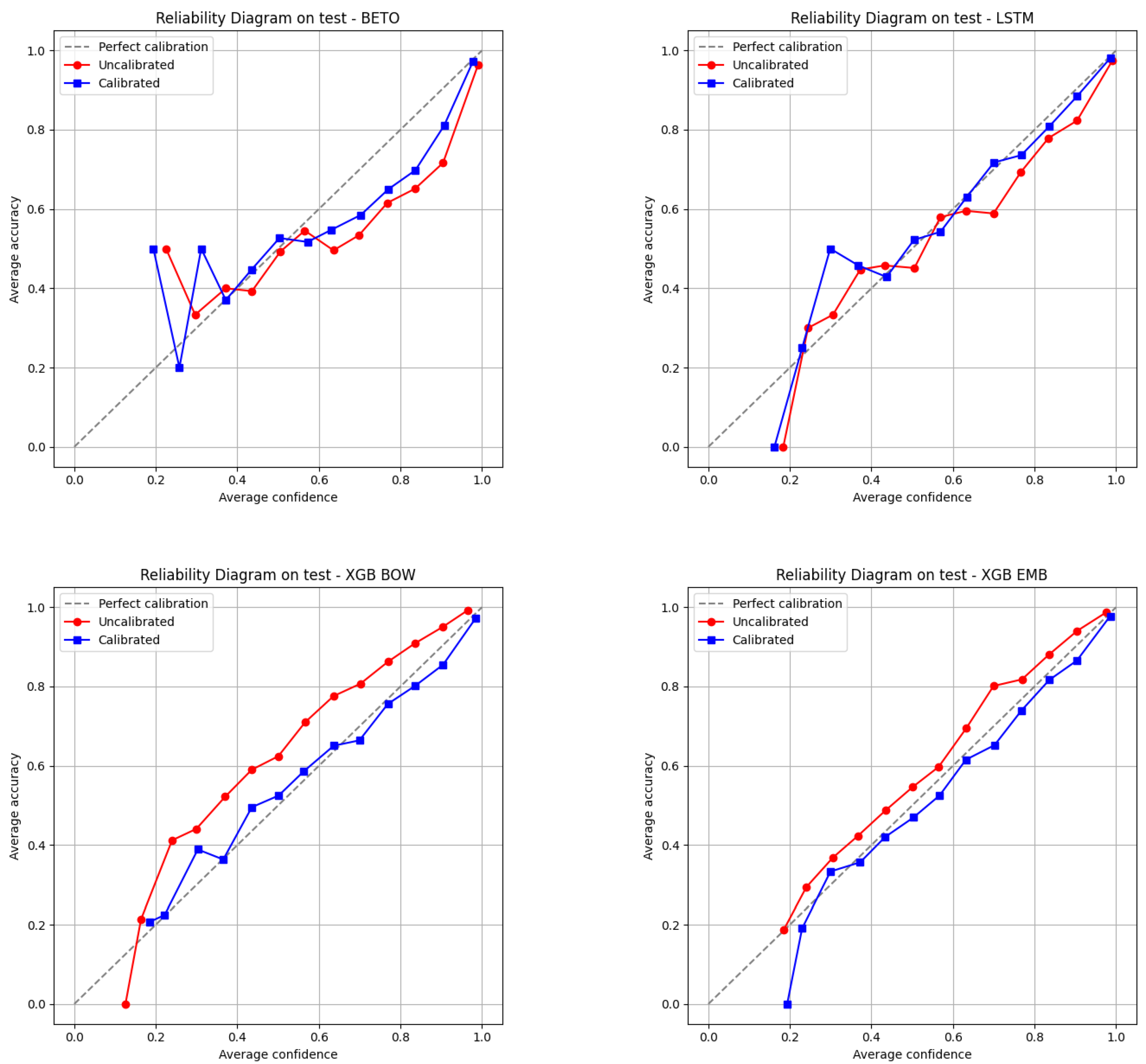
5.3. Selection Criteria Based on SoftMax Output

Both XGBoost and neural network architectures use SoftMax normalization (SoftMax normalization was applied externally to the XGBoost logits to generate class probabilities consistent with the neural network outputs), which maps each class to a value between 0 and 1. The SoftMax function is defined as

$$p_i={\displaystyle \frac{e^{z_i}}{{\sum }_j{e}^{z_j}}}$$

(5)

where $z_i$ denotes the logit (raw score) for class i, and $p_i$ is the normalized probability assigned to class i.

The predicted class for each record corresponds to the one with the highest SoftMax value. This value can be interpreted as an indicator of certainty and used to distinguish records with a higher or lower likelihood of being correctly predicted. Given the strong correlation between prediction accuracy and the certainty indicator, it is possible to define a threshold that separates records to be coded automatically from those that require review by an expert coder. This threshold is determined by the trade-off between production rate and accuracy—two factors that typically move in opposite directions; increasing one often leads to a decrease in the other [19,20].

The approach of this work is precisely to leverage the certainty indicator by establishing a threshold that minimizes manual effort while maintaining a level of accuracy considered acceptable. It is important to note that SoftMax is not a probability, so the threshold does not necessarily reflect the model’s performance in production. To perform this, a calibration adjustment would be required. The approach proposed here does not aim to use the cutoff score as a predictor of performance. Instead, the SoftMax value is used as a ranking variable to order the records, which then allows for splitting the data based on an empirical assessment of performance, as illustrated in Figure 2 in Section 6.2. In line with this approach, Section 6.3.2 on implementation presents results from the empirical evaluation of the model on the first data batches received during the survey collection, which allows for the establishment of a cutoff threshold.

In summary, if the threshold were used to estimate the model’s performance for records above the chosen value, SoftMax would not be a reliable indicator. Instead, this study uses the SoftMax value solely to rank the dataset and define a percentile-based threshold, after which the model’s empirical performance is evaluated. Nevertheless, to ensure that using a calibrated SoftMax score does not alter the conclusions, several experiments—presented in Appendix B—were conducted. These show that the calibrated SoftMax scores, following the procedure proposed by Guo et al. [21], yield nearly identical results.

6. Results

6.1. Model Comparison

This section presents the test set results for the three algorithms evaluated: XGBoost (BOW and word embeddings), an LSTM neural network with embeddings, and fine-tuning of the BETO transformer. The aim is to compare deep learning approaches with a machine learning-based boosting algorithm. It is worth mentioning that the XGBoost modality with a word embeddings representation corresponds to a hybrid option, since it combines a traditional algorithm with preprocessing that includes vectors that have been trained with a deep learning model.

Table 4. Performance metrics for XGB-BOW, XGB-EMB, LSTM, and BETO. XGB-BOW and XGB-EMB refer to gradient boosting models using bag-of-words (BOW) and embeddings (EMB), respectively. LSTM is a recurrent neural network, and BETO is a transformer-based model pretrained on Spanish text. Metrics were computed on the test set.

Metric/Model	XGB-BOW	XGB-EMB	LSTM	BETO
Accuracy	0.854	0.872	0.914	0.922
Precision (macro)	0.830	0.821	0.904	0.915
Recall (macro)	0.761	0.773	0.858	0.871
F1-Score (macro)	0.781	0.790	0.860	0.880
Precision (weighted)	0.856	0.871	0.914	0.923
Recall (weighted)	0.854	0.872	0.914	0.922
F1-Score (weighted)	0.852	0.870	0.913	0.922
Eval Loss	0.529	0.412	0.288	0.304
Support	10,126	10,126	10,126	10,126

shows the test results for the three models: XGBoost (BOW and word embeddings), an LSTM network, and a Spanish-language transformer model known as BETO. The goal is to evaluate the performance of deep learning approaches represented by the two neural network architectures against Extreme Gradient Boosting, a boosting algorithm known for its strong performance in classification tasks.

The accuracy metric quantifies the proportion of correct predictions among the total number of cases evaluated. precision is the ratio of true positives to predicted positives, and recall is the ratio of true positives to actual positives. These metrics can be computed as follows:

$$\begin{array}{c}\hfill Accuracy={\displaystyle \frac{TP+TN}{TP+TN+FP+FN}}\end{array}$$

(6)

$$\begin{array}{c}\hfill Presicion={\displaystyle \frac{TP}{TP+FP}}\end{array}$$

(7)

$$\begin{array}{c}\hfill Recall={\displaystyle \frac{TP}{TP+FN}}\end{array}$$

(8)

where $TP$ represents true positives, $TN$ represents true negatives, $FP$ represents false positives, and $FN$ represents false negatives. The F1-score combines precision and recall into a single metric by computing their harmonic mean. It is especially useful for imbalanced classification problems:

$$\mathrm{F}1\text{-}\mathrm{Score}={\displaystyle \frac{2·\mathrm{Precision}·\mathrm{Recall}}{\mathrm{Precision}+\mathrm{Recall}}}$$

(9)

The F1-score ranges from 0 (worst) to 1 (perfect).

The metrics consistently show that the deep learning algorithms (LSTM and BETO) outperform XGBoost. In the case of the accuracy metric, the deep learning approaches exceed XGBoost with BOW representations by approximately six percentage points. It is interesting to note that representing texts using word embeddings improves XGBoost’s performance by approximately 2 percentage points, using the accuracy and F1-score metrics as a reference.

Regarding the comparison between LSTM and BETO, the data show that BETO achieves higher performance across all metrics; however, the difference is small. When comparing performance at the class level (see

Table 5. F1-score for the six main crime classes. XGB-BOW and XGB-EMB refer to gradient boosting models using bag-of-words and embeddings, respectively. LSTM is a recurrent neural network, and BETO is a transformer-based model pretrained on spanish text. Metrics were computed on the test set.

Crime/Model	XGB-BOW	XGB-EMB	LSTM	BETO
Fraud/swindling	0.895	0.913	0.931	0.955
Bank fraud	0.912	0.930	0.948	0.960
Assaults and injuries	0.806	0.807	0.901	0.913
Domestic burglary	0.864	0.860	0.896	0.890
Vehicle vandalism	0.874	0.886	0.932	0.940
Household vandalism	0.845	0.891	0.931	0.946

), this pattern holds: BETO and the LSTM network perform similarly, both clearly outperforming XGBoost.

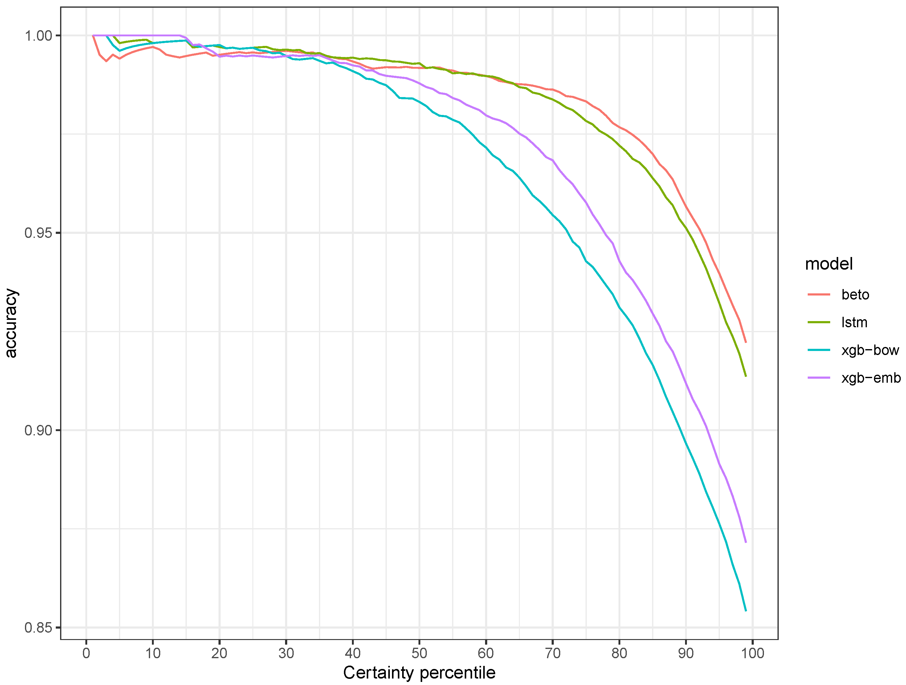
6.2. Model Certainty

As mentioned in Section 5, the certainty scores returned by the models can be used to compute performance metrics across different subsets of the dataset. Specifically, percentiles are generated from the certainty indicator to evaluate performance throughout the dataset. This strategy relies on the idea that the data can be partitioned in such a way that the model handles the portion where it performs best, while more complex cases are left to be coded by expert human coders.

Figure 2 contrasts the certainty indicator (x-axis) with the accuracy metric (y-axis). On the x-axis, the data are grouped into certainty percentiles, ordered from left to right from the highest to the lowest certainty. For each point, the cumulative proportion of correct predictions over the total number of observations considered up to that percentile is estimated (that is, the cumulative number of correct predictions up to the i-th percentile divided by the cumulative total of observations up to the i-th percentile). In this way, the figure shows how the model’s accuracy varies as a function of its certainty.

Overall, the three models show similar performance, with accuracy levels close to 100% in the top percentiles. Around the 30th percentile, a gap begins to emerge between XGBoost (BOW and embeddings) and the deep learning models. While the latter also show a decline in performance, it is less pronounced than that of XGBoost. It is also worth noting that in the higher percentiles (65 and above), BETO exhibits slightly better performance than the LSTM network, which is consistent with the overall results reported in Table 4. Finally, the comparison between the two XGBoost implementations shows that from the 30th percentile onwards, replacing BOW with a word embeddings representation improves predictions.

It is interesting to observe the shape of the curves. The first percentiles that are automatically coded show very low error rates, but these increase at an accelerating pace. Thus, moving from 0% to 10% automated coding introduces only a small error, whereas increasing automation from 70% to 80% results in a significantly higher error. This can also be interpreted in reverse: the cost of improving coding quality through manual work is increasing, as beyond a certain point, the marginal benefit of manual coding yields only minimal gains in accuracy.

6.3. The Proposed Workflow

6.3.1. Model Selection

The first step in implementing the new workflow was the selection of the model to be used. The results presented in the previous section indicate that BETO is the architecture that achieves the highest performance; therefore, if maximizing accuracy were the only consideration, BETO would be the preferred choice. However, when resource usage is also taken into account, the LSTM network emerges as the most appropriate alternative, given the available computing infrastructure.

Since BETO requires a GPU to operate optimally, resource usage becomes a critical factor. The National Statistics Institute does not have access to graphics processing units (GPUs) for deploying production services, which means that if BETO had been selected, the model would have had to run on a CPU—resulting in performance issues.

Table 6. Average processing times for BETO and LSTM with 500 observations.

Device	Avg. BETO Time (s)	Avg. LSTM Time (s)
GPU	0.701	-
CPU	82.370	1.201

Note: Processing times for BETO and LSTM. The results represent the average of 100 iterations on a randomly selected set of 500 records. The GPU test was carried out using an Nvidia RTX 4090 graphics card, while the CPU test was conducted on an 8-core Intel i7-7700 processor (3.60 GHz).

compares the execution time of BETO with and without a graphics processing unit (GPU). Predicting 500 records takes only 0.7 s on a GPU, whereas the same task takes 82.4 s on a CPU—roughly 100 times slower. Since the LSTM model produces comparable results, it was selected for deployment, prioritizing faster response times over marginal gains in accuracy.

6.3.2. Processing Changes

For the new crime coding workflow, an API was developed to enable programmatic queries for crime classification. These queries consist of sending text strings to the API, which returns crime codes along with a certainty score indicating the likelihood that the classification is correct, based on a previously trained model. The purpose of using such a service is to abstract the internal complexity of the crime classification model. From the user’s perspective, it is only necessary to think in terms of inputs (texts) and outputs (codes and certainty). In this way, the API can be seamlessly integrated into the workflow, helping to optimize the process without adding unnecessary complexity.

To evaluate the performance of the API within the new workflow, an initial trial period was defined with the aim of generating evidence on its accuracy. The trial covered the first two data extracts from ENUSC 2024, out of a total of eight scheduled during the data collection period (October to December 2024). In these first two extracts, all records were coded both by the API and by business analysts. Discrepancies were then reviewed by a senior analyst and/or coordinator.

Based on the results from these two extract cycles, certainty thresholds were established to determine when the API reliably confirms the crime code assigned during data collection. The focus was on identifying cases where the API’s classification matches both the code from field collection and the one assigned by a business analyst. Since the vast majority of classifications from fieldwork are correct, the first step centers on confirming these codes—an approach that allows most of the narrative volume to be cleared efficiently.

Establishing certainty thresholds for the API based on “easy” classifications makes it possible to define rules for delegating coding tasks to the API, aiming to maximize coverage and minimize errors. More complex cases, in turn, are handled by an analyst.

Table 7. Thresholds used in production. Accuracy values were calculated within the subset of data with certainty values above the established threshold—that is, before applying the business rules related to the detection of relevant strings.

Crime	Certainty Threshold	Auxiliary Variables	Relevant Terms	Accuracy  (%)
Vehicle vandalism	0.88	Reference period	intent, trat, rob, and others identified by the analyst	92.8
Domestic burglary	0.86	Reference period, value of stolen goods	intent, trat, door, gate, open, and others identified by the analyst	96.7
Household vandalism	0.85	Reference period	intent, trat, rob, and others identified by the analyst	81.8
Bank fraud	0.79	Reference period, stolen goods	intent, trat, and others identified by the analyst	96.8
Fraud /swindling	0.95	Reference period, value of stolen goods	intent, trat, and others identified by the analyst	96.5
Assaults and injuries	0.78	Reference period, relationship with responsible party	Family, couple, intrafamily, etc.	95.5

presents the thresholds for each crime category and the accuracy achieved for records that exceed those thresholds. While the model has a high average accuracy, its performance is not equal across all classes. Because of this, differentiated thresholds were established, which allows us to take advantage of what the model performs well and support it with manual coding for the records it does not classify as effectively.

To further strengthen the process, two versions of the model available through the API were used: one with 15 categories and another with 16. While these models are highly consistent, they do not always produce the same result—particularly in more challenging classification cases. It was therefore determined that a code is only confirmed when both models agree with the classification assigned during data collection. Finally, it is important to note that the certainty threshold is specific to each of the six crime types that include narratives. These thresholds were defined based on the model’s accuracy during the first two trial cycles (out of a total of eight data extract cycles).

Once the thresholds for delegating confirmations to the API were defined, a new workflow was established that integrates the model into the process. This workflow delegates to the API the classification of narratives with a high certainty score (above the previously defined thresholds) and that do not present risk attributes based on crime characterization variables or relevant terms within the narratives.

High certainty refers to cases in which both models deployed in production agree that the crime assigned by the interviewer is correct, with a certainty level above a predefined threshold. Risk attributes, on the other hand, refer to situations where a record shows variables that suggest a possible misclassification in the characterization (e.g., no loss reported) or includes terms that may indicate a misclassification (e.g., “intent”, “trato/a”, “roba/o”). In other words, only those cases that agree with the interviewer’s classification, show a high likelihood of accuracy, and do not exhibit signs of potential misclassification are delegated to the API. This approach follows the guidelines of other INE classification APIs (such as the CIUO 08.CL classification model), which recommend manually reviewing “difficult” cases and delegating “easy” ones.

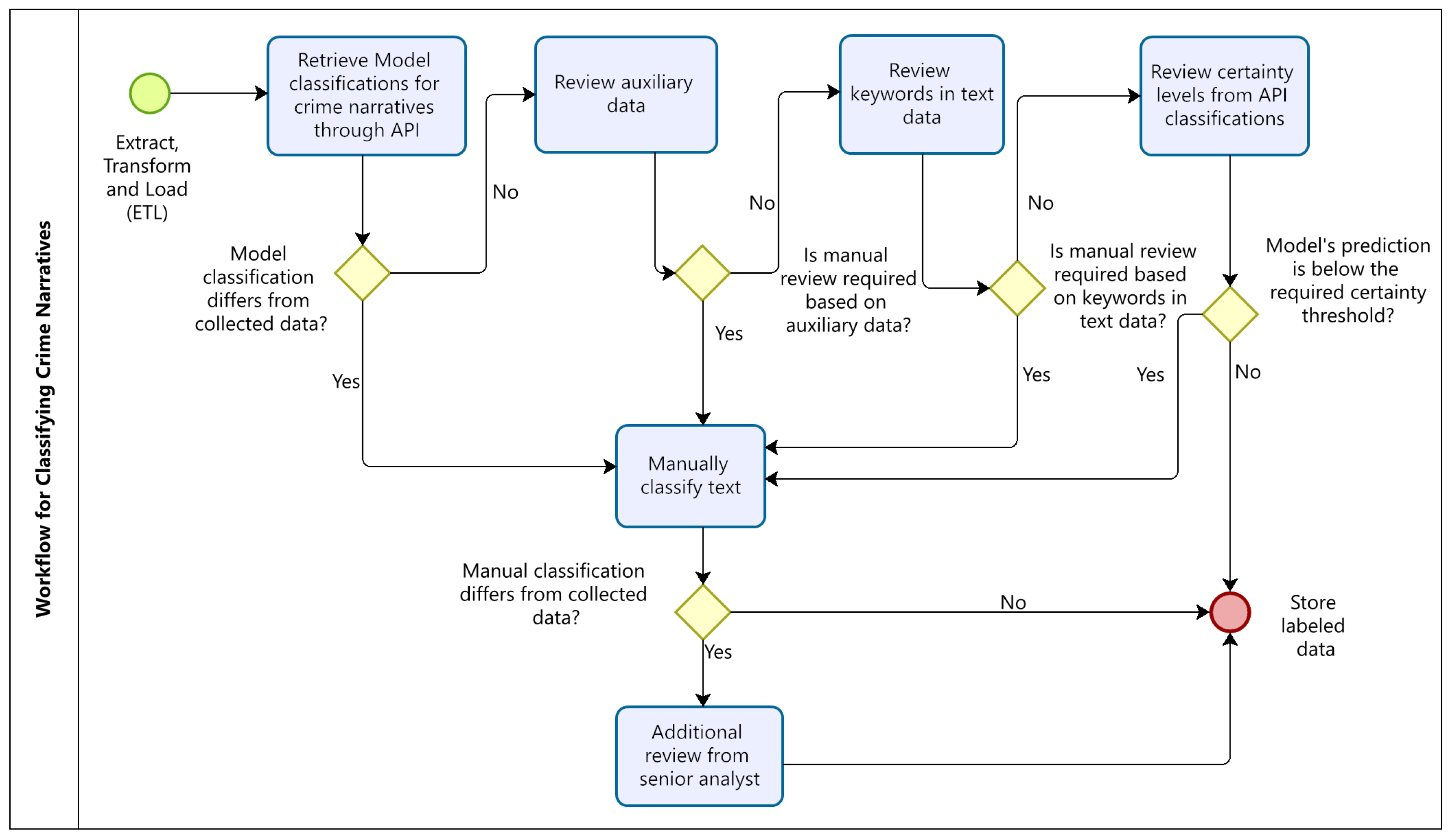
Figure 3 illustrates the complete process, based on a generic data extract. After integrating the downloaded data, a query is sent to the API, and the resulting classification is added as an additional column. Following the automated workflow, if the API’s classification matches the interviewer’s, if auxiliary variables raise no alerts, if no relevant terms indicate a potential issue, and if the narrative falls below the risk threshold, then the case does not require human review and the original field classification is retained.

Conversely, if any of these checkpoints in the workflow trigger an alert—whether due to a mismatch between the API and the field code, the presence of a specific value in an auxiliary variable, the detection of relevant terms, or the certainty score falling below the predefined classification threshold—the narrative is flagged for manual review.

Finally, it is important to note that if an analyst’s review results in a disagreement with the field-assigned code, an additional review is triggered. In such cases, a senior analyst or team coordinator must confirm whether the change to the original classification is warranted. In this sense, the workflow is designed to achieve an optimal balance between maximizing the use of the API and minimizing potential classification errors—whether from fieldwork or the API itself.

As shown in

Table 8. Manual and automatic review percentages in ENUSC 2024.

Crime	API	Manual
Vehicle vandalism	74.7%	25.3%
Domestic burglary	55.9%	44.1%
Household vandalism	63.3%	36.7%
Bank fraud	78.5%	21.5%
Fraud	64.2%	35.8%
Assault and injuries	48.9%	51.1%
Total	68.4%	31.6%

, for the 2024 ENUSC version—considering cycles three through eight (excluding the first two trial cycles)—a significant reduction in manual workload was achieved. Out of a total of 4591 narratives during this stage, 3141 were delegated to the API following the previously described workflow. Considering the six types of crimes that still include narratives in ENUSC, this represents a 68.4% reduction in the need for manual review.

Once the coding process under the new workflow was completed, a final quality control was implemented, involving a random review of approximately 10% of the records delegated to the API within each crime type. The results of this exercise are presented in

Table 9. Random review of records assigned to the API in ENUSC 2024.

Crime	Audited	Discrepancies	API
Vehicle vandalism	82	0	781
Domestic burglary	35	0	340
Household vandalism	29	0	276
Bank fraud	109	0	1029
Fraud	58	2	558
Assault and injuries	18	0	157
Total	331	2	3141

. Out of a total of 331 reviewed cases, only 2 discrepancies were found between the API and the human analyst’s judgment. However, these two cases were not classification mismatches; rather, they involved narratives that lacked sufficient information to allow for any classification (“insufficient” status), whereas the API had—by chance—assigned the field classification. This corresponds to an error rate of just 0.6%, which is remarkably low and demonstrates that the workflow is effective in isolating complex cases while reliably delegating the simpler ones to the API, resulting in significant labor savings with minimal error.

7. Conclusions

This work presents a successful case of applying deep learning for the automatic coding of text in the context of official statistics production. Unlike previous experiences focused on economic activity and occupation data, this case applies deep learning to crime data.

The tests conducted show that the deep learning approach outperforms a more “traditional” algorithm such as XGBoost. An interesting finding is that even a more traditional approach based on an algorithm like XGboost can take advantage of deep learning, incorporating a text representation based on word embeddings.

Among the deep learning options evaluated, the best-performing architecture was BETO, a large language model (LLM) fine-tuned for the task. However, its use in production was ruled out. Due to computing infrastructure constraints, a simpler deep learning model was selected. The LSTM network delivered slightly lower performance than BETO but requires significantly fewer resources, as it does not depend on GPU processing. In this regard, a trade-off was made: accepting a small decrease in accuracy in exchange for a substantial reduction in computational cost. This highlights the importance of balancing available infrastructure with the choice of model to be deployed.

The integration of the model into the ENUSC workflow greatly benefited from the availability of an API, which allows access to predictions without requiring business experts to have deep learning knowledge or advanced programming skills. This enabled ENUSC analysts to focus entirely on the challenge of developing business rules to operationalize the model and incorporate prediction outputs into their regular workflow.

Deploying the model into production has led to substantial savings in human resources. Of the 4591 narratives included in the review phase, 3141 were delegated to the API, freeing up time for the business team to focus on improving quality in other stages of the process. One of the most important conclusions of this work is the value of not fully replacing manual work. The results derived from the certainty indicator suggest that, given the current model performance, it is advisable to split the dataset—allowing the algorithm to handle part of the workload while assigning the more complex cases to human coders. As models improve, manual intervention may decrease; however, given the tools and capacities currently available at INE, maintaining some level of manual review remains necessary to uphold the institution’s high-quality standards.

One of the main limitations of this work relates to the computational trade-offs associated with model selection. While lightweight models offer a practical alternative for statistical offices with limited infrastructure, they do so at the cost of some predictive performance, particularly in more complex cases. However, these edge cases—where model certainty is low—are precisely the ones that should remain under manual review, which aligns with the intended use of automation as a complementary, not substitutive, tool.

A second limitation stems from the sensitive nature of the data used. Because crime narratives involve confidential personal information, the underlying microdata cannot be publicly released. This constraint limits external validation and open experimentation, which are essential for broader methodological development and cross-institutional collaboration.