Article

Requiem for Olympic Ethics and Sports’ Independence

Dipartimento di Scienze per la Qualità della Vita, Università di Bologna, C.so d’Augusto 237, 47921 Rimini, Italy
Stats 2025, 8(3), 67; https://doi.org/10.3390/stats8030067
Submission received: 11 June 2025 / Revised: 19 July 2025 / Accepted: 23 July 2025 / Published: 28 July 2025
(This article belongs to the Special Issue Ethicametrics)

Abstract

This paper suggests a theoretical framework to summarise the empirical literature on the relationships between sports and both religious and secular ethics, and it suggests two interrelated theoretical models to empirically evaluate the extent to which religious and secular ethics, as well as sports policies, affect achievements in sports. I identified two national ethics (national pride/efficiency) and two social ethics (social cohesion/ethics) by measuring achievements in terms of alternative indexes based on Olympic medals. I referred to three empirical models and applied three estimation methods (panel Poisson, Data Envelopment, and Stochastic Frontier Analyses). I introduced two sports policies (a quantitative policy aimed at social cohesion and a qualitative policy aimed at national pride), by distinguishing sports in terms of four possibly different ethics to be used for the eight summer and eight winter Olympic Games from 1994 to 2024. I applied income level, health status, and income inequality, to depict alternative social contexts. I used five main religions and three educational levels to depict alternative ethical contexts. I applied country dummies to depict alternative institutional contexts. Empirical results support the absence of Olympic ethics, the potential substitution of sport and secular ethics in providing social cohesion, and the dependence of sports on politics, while alternative social contexts have different impacts on alternative sport achievements.

1. Introduction

There are many theoretical papers on ethics of sport (i.e., individual rules to ensure fairness in competitions); for example, Devine [1] on excellence, Park et al. [2], Van Der Hoeven et al. [3], Moriconi & Almeida [4], and Csató [5] on match-fixing, Devine [6] on leadership, Constandt et al. [7] on illegal gambling, and Lewandowski [8] on the cornerman and boxer interactions. There are few empirical papers on the ethics of sport (i.e., reliable factors favouring individual fair behaviours). In particular, Tabar et al. [9] focus on the moral responsibility of sport societies by referring to 13 interviews with experts (i.e., a small sample); Spruit et al. [10] focus on moral behaviours on the playing field by referring to 27 previous studies (i.e., a meta-analysis).
There are many theoretical papers on ethics for sport (i.e., social rules to ensure fairness in access to competitions); for example, Ryba et al. [11] on social inclusion, Spowart [12] on single-motherhood, Ogunrinde [13] on black girls, Krieger et al. [14] and Zakhem & Mascio [15] on drugs, Hochstetler et al. [16] and Kirkwood [17] on doping, Cooper [18] and McCalla [19] on testosterone, Pike [20], Hamilton et al. [21], Shaw et al. [22], and Ordway et al. [23] on transgender issues, and Frias & Torres [24] on cloning horses in polo. There are few empirical papers on ethics for sport (i.e., reliable factors to ensure fair access socially). In particular, Kulkarni et al. [25] focus on the personal development of disadvantaged youths, although their dataset is based on 15 qualitative media studies (i.e., a meta-analysis).
There are many theoretical papers on ethics to sport (i.e., on government approaches or athletes’ attitudes toward sports); for example, Twietmeyer et al. [26] on Christian ethics, Tak et al. [27] on Confucianism, and Frias [28] on Protestant ethics. There are few empirical papers on ethics to sport. In particular, De Waegeneer et al. [29] focus on moral intentions, although their dataset consists of 171 participants (i.e., a small sample).
Note that research on ethics to sport has recently focused on sport integrity (i.e., sport stakeholders upholding a range of moral values such as honesty, sportsmanship, respect, and trustworthiness in fulfilling their sport organisational roles, namely, professional responsibility, as well as within wider society, namely, personal responsibility, to ensure a safe, fair, and inclusive on-field and in-competition activity) by taking an individual and psychological perspective (e.g., [30,31]).
There are many theoretical papers on ethics through sport (i.e., social or individual ethics acquired from sports); for example, Avner et al. [32] on sports work, Pankow et al. [33] on psychological skills, Aggerholm [34] on defiance, Constantin et al. [35] on sports integrity, and Debognies et al. [36] on disadvantaged youths. There are few empirical papers on ethics through sport. In particular, Uğraş et al. [37] focus on dedication by relying on a small sample of 237 amateurs (i.e., a small sample), and Quartiroli et al. [38] focus on self-care by referring to 1837 research records (i.e., a meta-analysis).
Note that research on ethics through sport has recently focused on sport education (i.e., sport students learning a range of moral values such as patience, tolerance, friendship, mutual respect, and excellence to address the most common threats to sustainable development, including global economic polarisation, deepening of social inequalities, neglect of human rights, and destruction of the global environment), by taking an international and social perspective (e.g., [39,40]).
In other words, four main gaps can be identified in the literature: the reliance on small samples, the application of meta-analyses, the focus on either religious or secular ethics, and the consideration of either ethics to or ethics through sport.
Note that Gunnell et al. [41] criticise the common use of meta-analysis in the sports literature.
The purpose of this paper is to bridge these four gaps by suggesting a theoretical framework (GOAL 1) to summarise the empirical literature on the relationships between both ethics to and ethics through sport and both religious and secular ethics (REL, SEC), and by suggesting two interrelated theoretical models (GOAL 2) to empirically evaluate to what extent REL or SEC as well as sport policies affect achievements in sport ethics, applying panel data analyses at a country level to Olympic Games as a case study of global ethics to and through sport (see Table 2 for the list of all acronyms). To do so, I identified two national ethics (i.e., national pride, national efficiency) and two social ethics (i.e., social cohesion, social ethics) by properly measuring achievements in terms of alternative indexes based on Olympic medals (i.e., gold medals per capita, GM, total medals per capita, TM, winning the gold match final, and winning the bronze match final BM). Moreover, I consistently referred to three empirical models and applied three estimation methods (i.e., panel Poisson Analysis PA, Data Envelopment Analysis DEA, and Stochastic Frontier Analysis SFA) by focusing on eight alternative estimations. Finally, I originally introduced two sport policies (i.e., a quantitative policy based on the total number of athletes and disciplines aimed at social cohesion, POLC, and a qualitative policy based on the variations’ coefficient of athletes across disciplines aimed at national pride, POLP), by distinguishing sports in terms of four possibly different ethics (i.e., direct games DIR, direct games with contact, DIRcon, direct games in teams, DIRtea, indirect games, IND) to be used for both summer and winter Olympic sports.
Note that I referred to income level, health status and income inequality (i.e., Gross Domestic Product per capita, GDP, Healthy Life Expectancy at Birth, HLEB, and the Gini Index, INE) to depict alternative social contexts, as used in the literature (e.g., [42]). Moreover, I firstly introduced five main religions (i.e., percentages of believers in Buddhism BUD, Christianity CHR, Hinduism, HIN, Islam, ISL, Judaism, JUD) and three educational levels (i.e., primary, GEP, secondary, GES, and tertiary, GET, gross enrolment rates) to depict alternative ethical contexts. Finally, I relied on country dummies to depict other country peculiarities, as used in the literature (e.g., [43]). Thus, the purpose of the present study is to estimate to what extent qualitative or quantitative sport policies are consistent with national or social ethics in alternative social and ethical contexts, where no statistically significant relationships between sport achievements and policies or ethics means that the Olympic ethics (i.e., the important thing in Olympic Games is not so much the winning but taking part, for the essential thing in life is not conquering but fighting well) prevail since my sample includes all athletes participating in Olympic Games from 1994 to 2024 (i.e., eight winter and eight summer editions).
Note that research on the Olympic values (e.g., [44,45]) has shown that the above definition of the Olympic ethics (i.e., fighting well by improving yourself—excellence, rather than winning dishonestly by trying to destroy others—disrespect) represents a popular, although concise, meaning of the Olympic spirit (i.e., a life philosophy grounded in the balanced development of the body and mind, joy emanating from hard work, the educational value of setting an example for others, patience, tolerance, friendship, equality, social responsibility, and respect for universal and fundamental human principles). Here, I will focus on the Olympic ethics to show that governments pursue well-defined objectives (i.e., national pride and social cohesion). Out of scope is the International Olympic Committee, which pursues the spread of the Olympic spirit (i.e., Olympism in sport integrity and sport education).
In other words, the research questions can be summarised as follows: RQ (1) Is Olympic ethics still relevant? RQ (2) Do different religious and secular ethics impact on sport achievements? RQ (3) Do different institutional contexts characterising different countries affect sport achievements? RQ (4) Is politics neutral toward sports?
Note that the focus on national or social ethics excludes specific insights into individual strategies and socio-ethical interactions at the individual level, which could be ideally obtained by developing a game theoretical model.
In addition to the theoretical framework for summarising the empirical literature on the relationships between sports and both religious and secular ethics, the topical contribution of the present paper is twofold: it finds that REL (i.e., Buddhism, Hinduism, Islam) and SEC (i.e., secondary education) have significantly larger negative and positive impacts on sport achievements, respectively, when governments pursue national pride rather than social cohesion; it finds that income level always positively impacts on GM only, health status always negatively affects both GM and TM, and income inequality always negatively impacts on TM only. In addition, the methodological contribution of the present paper is twofold: it shows that the Poisson Model is incorrect, and it shows that DEA is incomplete.
Note that NBIC technologies (i.e., nanotechnology, biotechnology, information technology, and cognitive science) are not conducive to social cohesion (e.g., [46]). Moreover, I will disregard studies on, and close to, the literature on sports medicine (e.g., Zurc [47] on the acceptance of health risks by athletes), sports management (e.g., Ribeiro et al. [48] on Olympic Games), sports education (e.g., Bakhtiyarova et al. [49] on ideals, values, and principles of Olympism), and sports regulation (e.g., Muñoz et al. [50] on governance of sports organisations). Finally, doping and testosterone are against national pride (e.g., [51]).
The structure of the present paper is as follows. Section 2 suggests the comprehensive theoretical framework by introducing an output index and two methodologies to complete the literature. Section 3 details the three empirical models, by presenting consistent formulas for PA, SFA and DEA in Section 3.1, Section 3.2 and Section 3.3, respectively. Section 4 constructs the dataset, considering summer and winter Olympic Games from 1994 to 2024. Section 5 details the estimations of the three empirical models, by presenting comparable results from PA, SFA, and DEA in Section 5.1, Section 5.2 and Section 5.3, respectively. Section 6 discusses the achievements of the three empirical models combined with respect to the research questions, highlighting the strengths and weaknesses of the methodology suggested in the present paper. Section 7 discusses the achievements of SFA with respect to the research purposes, highlighting the topical and methodological successes of the present paper.

2. Methods: The Theoretical Framework

From the literature on ethics to and through sport, one can obtain four objectives (national pride, social cohesion, social ethics, and national efficiency) (e.g., [43]), three indexes (gold medals, total medals, efficiency scores) (e.g., [52]) and two methodologies (PA and DEA) (e.g., [53]). I will complete this theoretical framework by introducing one index and two methodologies: ∆G = GM − SM and ∆B = BM − WM to depict social ethics (i.e., rewarded hard work, dedication and resilience), where SM, BM and WM stand for silver, bronze and wood (i.e., if the bronze match final is lost) medals, respectively; SFA with and without country dummies to represent the relationships between ethics and sports, by considering and disregarding country specificities, respectively.
Next, from the literature on ethics to and through sport, one can obtain three main independent variables (GDP, HLEB and INE) (e.g., [42]). I will complete this theoretical framework with two sport policies (POLP, POLC) and two ethics (REL, SEC). I will distinguish sports in terms of four different ethics or categories, common to winter and summer Olympic Games: direct competitions with contact (6 sports), direct competitions (18 sports), direct competition by teams (11 sports), indirect competitions (13 sports) [54] (See Supplementary Materials S1 for the detailed lists of sporting disciplines for each category). Thus, I will define POLP (i.e., a qualitative assessment of the governmental sport policy assumed to be directed to national pride by effectively using monetary and non-monetary resources to win as many GM as possible) as the variations’ coefficient of athletes across disciplines and POLC (i.e., a quantitative assessment of the governmental sport policy assumed to be directed to social cohesion by effectively using monetary and non-monetary resources to win as many TM as possible) as the total number of athletes across disciplines [55]. Note that I used the variations’ coefficients across categories to standardise with respect to the number of athletes for each country since there is a maximum given number of athletes for each discipline and the number of disciplines for each category is fixed. Moreover, I will distinguish REL (i.e., percentage of believers) into five main religions: BUD, CHR, HIN, ISL, and JUD (i.e., percentages of believers in Buddhism, Christianity, Hinduism, Islam, and Judaism). Finally, I will distinguish SEC (i.e., percentages of educated people) into three education levels: GEP, GES, and GET (i.e., primary, secondary, and tertiary gross enrolment rates).
Table 1 summarises the governmental objectives, output indices, input variables, and methods in a theoretical framework by stressing the expected positive or negative impacts of different input variables on alternative output indices.
Note that some impacts are expected to be positive. For example, a larger income level (GDP) is likely to favour larger funds for sports [56], although I will identify which governmental objective is more affected by the per capita income level. Similarly, a larger SEC is likely to make sport funds more productive [57], although I will specify which education level is more productive. Moreover, some impacts are expected to be negative. For example, a negative REL represents the absence of confrontative ethics in most religions [58], although I will specify which religions are less confrontative. Finally, some impacts could be either positive or negative, depending on the governmental objective under consideration. For example, a positive impact of income inequality (INE) could depict larger sport achievements in countries with more inequality due to the larger social redemption attached to sport [59], but a negative impact of INE could depict larger sport achievements in more equal countries, due to more opportunities for gifted people [60]. Similarly, I will use total population to standardise medals (i.e., to compare small and large countries) rather than as an independent variable since finding an Olympic athlete is a matter of quality (i.e., gifted people) rather than of quantity (i.e., young people) [61,62]. Consequently, HLEB represents both the health status of the general population and the proportion of old people: a positive impact of HLEB depicts contexts where a better health status of the general population prevails over a larger set to choose young athletes, whereas a negative impact of HLEB depicts contexts where a larger set to choose young athletes prevails over a larger proportion of old people. All these expected impacts will be verified in Section 5.
Some methodological observations are noteworthy here. First, I did not use a dummy variable for the hosting country and a variable for the time trend to favour the comparisons of estimations from SFA and DEA, although Supplementary Materials S3 provides all estimations with these additional variables. I did not refer to democracy, population aged 20–34 years, freedom, or perceived corruption since they are not significant in the literature. I did not use weighted medals, since relative weights (e.g., 3, 2, 1 for gold, silver and bronze medals, respectively) are arbitrary. I did not refer to sport traditions or climate conditions, since they are depicted by country dummies. Second, in governmental sport policies, I did not distinguish countries where governments finance sports directly (e.g., governmental federations), countries where governments finance sports indirectly (e.g., athletes employed in specific armies), and countries where governments do not finance sports (e.g., athletes enrolled in private colleges). However, governmental objectives for sport are similar. In governmental sport policies, I did not distinguish professional from non-professional sports. However, individual ethics to sport are similar. Third, in SFA, countries without medals are excluded, whereas PA includes these countries [53]. However, sport achievements are assumed to be casual in PA (i.e., a stochastic process possibly dependent on some factors), whereas they are assumed to be pursued in SFA (i.e., a stochastic production function based on specified inputs). In SFA a single objective can be depicted as an independent variable, whereas in DEA, both single and multi-objective independent variables can be estimated [63]. However, SFA provides a complete ranking of countries in terms of efficiency, estimating the significance and value of all country dummies, whereas DEA provides a partial ranking of countries in terms of efficiency, by calculating shadow prices for some specified countries. Note that there is a limit to the number of participants, so large countries are undervalued in terms of per capita Olympic achievements. Moreover, POLC is a sufficient but not necessary condition for a sport diffusion at a national level, although it changes over time, and it also estimates the quality of sport federations (i.e., number of athletes in each category) as well as the quantity of sports (i.e., category with at least one athlete). Finally, the Gini Index measures an outcome of both REL and SEC ethics at a country level (i.e., many cultural and institutional contexts).

3. Methods: The Empirical Models

From the literature on ethics to and through sport, one can obtain 2 methodologies (PA, DEA) (e.g., [53,63]). I will discuss PA in Section 3.1 and DEA in Section 3.3, completing these methodologies by introducing SFA in Section 3.2. Indeed, comparing estimations from PA and from SFA will highlight whether achieving Olympic medals is better represented as a production or as a stochastic process, where both PA and SFA are developed within a random framework. The statistical significance of policies in PA will suggest that a production process should be preferred to a stochastic process (i.e., requiem of Olympic ethics and sports’ independence). Moreover, comparing SFA applied to single medals, sums of medals, or differences in medals will highlight which governmental objective is pursued. The statistical significance of some policies for some governmental objectives in SFA will highlight which policy is used for which objective. Finally, comparing estimations from SFA and from DEA will highlight some peculiarities of some specific countries, where SFA and DEA assume a random and a deterministic production function, respectively. The similar relative importance of the same policies for the same objectives obtained in DEA for single countries and in SFA for many countries will suggest that DEA could be applied instead of SFA for small datasets on a few countries (i.e., the focus on efficiency in a deterministic production function). Note that I will test DEA for the top 3 countries according to lexicographic and sum rankings over the 16 editions of the Olympic Games.

3.1. Poisson Analysis

The literature on PA applied to Olympic medals refers to the well-grounded theory of stochastically countable quantities: Prob(Y = y|x) = F(y, x β + ξ), where X is Poisson distributed with mean exp(z). In particular, the Poisson Model can depict the countable Olympic medals (Mi,t) within random-effects panel-data models as follows:
P r o b ( M i , t ) = α P O L P O L i , t + β G D P G D P i , t + β H L E B H L E B i , t + β I N E I N E i , t + β R E L R E L i , t + β S E C S E C i , t + ψ i
With
ψ i Γ 1 , ω
where Mi,t are the number of medals achieved by country i in year t and POLi,t is the sport policy implemented by country i in year t, whereas GDPi,t, HLEBi,t, INEi,t, RELi,t, and SECi,t are the observed values of income level, health status, income inequality, religious and secular ethics in country i in year t. Note that ψi is assumed to be i.i.d. such that exp(ψi) is gamma with mean 1 and variance ω to be estimated from the data. In other words, winning medals is depicted by the Poisson Model as a stochastic process possibly dependent on sport policies (i.e., POL) and socio-ethical contexts (i.e., GDP, HLEB, and INE as social variables, whereas REL and SEC as ethical variables).

3.2. Stochastic Frontier Analysis

SFA applied to Olympic medals refers to the well-grounded production theory: Y = f(X), where Y is the achieved production level and X is the vector of used production factors. In particular, SFA can depict the Olympic medals (Mi,t) within random-effects panel-data models as follows:
L n M i , t = α P O L L n P O L i , t + β G D P G D P i , t + β H L E B H L E B i , t + β I N E I N E i , t + β R E L R E L i , t + β S E C S E C i , t + D i + ζ i , t + ξ i , t
With
  ζ i , t N μ ,   σ u   a n d   ξ i , t N ( 0 ,   σ v )
where Ln is the natural logarithm and Di are dummy variables capturing the country’s specificities. Note that coefficients of production factors represent a constant returns to scale (CRS) or a decreasing returns to scale production functions if they sum up to 1 or to less than 1, respectively; ζi,t depicts the level of efficiency of observation i at time t (truncated at 0 with mean μ and variance σu); and ξi,t represents the idiosyncratic error (independently and identically distributed with mean 0 and variance σv) [64]. In other words, it is assumed a Cobb-Douglas production function M = f(POL) which can be shifted up or down by income level, health status, income inequality, religious and secular ethics, once the country specificities other than ethics are caught by the country dummy variables (i.e., all constant terms are assumed to be depicted by variables other than POL).

3.3. Data Envelopment Analysis

DEA applied to Olympic medals refers to the well-grounded production theory: Y = f(X), where Y is the achieved production level and X is the vector of used production factors. In particular, the (output-oriented and CRS) DEA can depict the production function for each country as follows:
M i n λ , θ , ε + , ε i n ε i + ε i
s . t . ε i + 0 , ε i 0 , λ i 0 , i n λ i = 1
θ P O L i , G D P i , H L E B i , I N E i , t , R E L i , S E C i X λ ε i = 0
Y λ + ε i + = M i , t
where the vector λ represents the reference weights to be attached to observations to identify the optimal solution, and θ is the efficiency score. Note that the same problem will not be estimated by replacing the constant with a variable or non-increasing returns to scale for lack of adequate observations in each country [65].
Next, the (output-oriented and CRS) DEA can depict the joint-production function for each country as follows:
M i n λ , θ , ε + , ε i n ε i + ε i
s . t . ε i + 0 , ε i 0 , λ i 0 , i n λ i = 1
θ P O L i , G D P i , H L E B i , I N E i , t , R E L i , S E C i X λ ε i = 0
Y λ + ε i + = G M i , t , S M i , t , B M i , t
where GM, SM, and BM are gold, silver, and bronze medals and represent additional outputs. Note that the assumption of weak disposability (i.e., changes in GM can possibly be obtained only by affecting SM and BM, changes in SM can possibly be obtained only by affecting GM and BM, and changes in BM can possibly be obtained only by affecting GM and SM) is consistent with the (almost always) presence of a single type of medal for each sporting discipline [66].
In other words, winning medals is depicted by DEA as a single or joint production process, possibly dependent on sport policies (i.e., POL) and socio-ethical contexts (i.e., GDP, HLEB, and INE as social variables, whereas REL and SEC as ethical variables).

4. Methods: The Dataset

Section 1 suggested the adoption of a representative individual perspective at the country level, Section 2 suggested 4 governmental objectives, 4 output indices, 6 input indices and 4 methodologies, and Section 3 developed 4 empirical models based on production and stochastic processes as theoretical models. In this section, I will describe the per capita variables used to estimate the 4 empirical models in alternative cultural and institutional contexts. In particular, the number of Olympic medals and the number of Olympic athletes for each discipline are obtained from the Olympic dataset (www.olympic.org, accessed on 10 July 2025). Moreover, REL is obtained from the World Religions dataset (www.worldreligions.org, accessed on 10 July 2025) as a sum of believers (percentages) in all religions, although REL will be detailed by focusing on the 5 main religions (i.e., Buddhism, Christianity, Hinduism, Judaism, and Islam) to measure alternative religious ethics. Finally, GDP per capita (in current USD), HLEB (Healthy Life Expectancy at Birth in years), INE (the Gini Index) and SEC (the sum of primary, secondary and tertiary gross enrolment rates in percentages) are obtained from the World Bank dataset (accessed on 10 July 2025), although the focus will be on secondary education to measure common secular ethics.
Note that I focused on income inequality, as fairness is the crucial ethical concept in sport, whereas I disregarded gender discrimination, as ethics to and through sport is the same for distinct male and female sporting disciplines.
Table 2 summarises the main statistics of the used variables by considering the summer and winter Olympic Games from 1996 to 2024 (8 winter and 8 summer editions). Note that the winter and summer Olympic Games were in the same year in 1992 and before 1992 [67].
Some methodological observations are noteworthy here. First, the number of medals and athletes for team sports is larger than for individual sports. Second, I used the average of the two previous values for each variable other than medals (i.e., for each independent variable), since the Olympic Games take place in the first months and in the middle months of the Olympic year for winter and summer editions, respectively. Third, I used the proportion of athletes across disciplines for each country in 2020 and also in 2024 since data for 2024 show medals and total athletes only.

5. Results

Section 3 suggested three empirical models (i.e., PA, SFA, and DEA) with SFA and DEA based on the same theoretical model (i.e., a production function at a country level), while Section 4 described the per capita variables to estimate the empirical models in alternative cultural and institutional contexts. In this section, I will estimate these empirical models by referring to the alternative objectives and indices summarised in Table 1. In particular, PA will be estimated in Section 5.1, while SFA and DEA will be performed in Section 5.2 and Section 5.3, respectively.
Table 3 summarises the performed estimations, by specifying the related Tables in the main text and in Supplementary Materials S1 and S2.

5.1. Poisson Analysis

Research question RQ (1) in Section 1 mentioned Olympic ethics. This subsection will test whether Olympic achievements can be depicted as a stochastic process. In particular, Table 4 and Table 5 present results for PA applied to GM and TM, respectively.
Table 4 shows that both policies are significant (i.e., a negative POLP suggests to focus on few disciplines to win GM; a positive POLC suggests to increase the number of Olympic athletes to win GM); GDP is positively irrelevant (as it was unexpected); HLEB is negatively significant (i.e., the access to a larger set to choose young athletes prevails over a better health status of the general population); INE is negatively significant (i.e., opportunities for a larger number of people prevail over greater needs of social redemption from sports, whenever the objective is winning GM); REL as a whole is negatively irrelevant (as it was expected); and SEC a whole is positively significant (as it was expected). Note that the significant CONS at 1.76 measures GM per million people.
Comparing Table 5 with Table 4 shows that GDP becomes positively significant (i.e., larger funding to sports is beneficial, whenever the objective is winning many medals); INE is now positively significant (i.e., greater needs of social redemption from sport prevail over opportunities for a larger number of people, whenever the objective is winning many medals); and SEC is now negatively significant (i.e., larger opportunities other than sports for a larger number of people due to a greater access to education is detrimental, whenever the objective is winning many medals). Note that the significant CONS at 4.22 measures TM per million people. Therefore, both policies (i.e., POLP, POLC) are significant for both objectives (i.e., GM and TM), so winning medals cannot be represented as a stochastic process. In other words, athletes are used by governments to pursue their objectives in alternative cultural and institutional contexts.

5.2. Stochastic Frontier Analysis

Section 5.1 showed that winning Olympic medals is not a stochastic process. This subsection will test whether Olympic achievements can be depicted as a production process by performing SFA. In particular, Table 6 and Table 7 present the linkages with Table 4 and Table 5 in Section 5.1 (i.e., PA with undetailed REL and SEC), Table 8, Table 9, Table 10 and Table 11 show the detailed estimations focused on POLC, Table 12, Table 13, Table 14 and Table 15 show the detailed estimations focused on POLP, and Table S2.1 for GM and Table S2.2 for TM in Supplementary Materials S2 present the linkages with Table 18 in Section 5.3 (i.e., DEA estimations for some countries with undetailed REL and SEC).
Comparing Table 6 with Table 4 shows that some significant results are confirmed (i.e., positive POLC, negative HLEB, negative INE, CONS at 1.936), some variables become significant (i.e., GDP), and some variables become non-significant (i.e., SEC). Note that decreasing returns to scale prevail (i.e., 0.803 − 0.063 < 1). Comparing Table 7 with Table 5 shows that some significant results are confirmed (i.e., positive POLC, negative HLEB, CONS at 3.467), some variables become significantly negative (i.e., INE), and some variables become non-significant (i.e., GDP and SEC). Note that constant returns to scale prevail (i.e., 1.080 − 0.075 ≈ 1). Therefore, winning Olympic medals is a production process, with decreasing and constant returns to scale for GM and TM, respectively. These results are corroborated by comparing goodness of fit obtained in PA and in SFA (Table A1 in Appendix A), since SFA always shows a better fit than PA. Similarly, the comparison of significance levels of coefficients for sport policies with original P values (based on dependence between hypotheses) and adjusted P values (based on independence of hypotheses) supports these results (Table A2 in Appendix A) since POLC confirms its statistical significance, whereas POLP becomes statistically significant with the three types of adjusted P values (i.e., List, Shaikh and Xu; Bonferroni; Holm).
Research questions RQ (2) and RQ (3) in Section 1 mentioned different religious and secular ethics as well as different institutional contexts. Table 8, Table 9, Table 10, Table 11, Table 12, Table 13, Table 14 and Table 15 specify 5 main religions for REL and 3 education levels for SEC, together with income level, health status and income inequality.
Comparing Table 8 and Table 9 with Table 6 and Table 7 shows that all significant results are confirmed (i.e., decreasing and constant returns to scale for GM and TM, respectively; GDP impacting on GM but not on TM; negative HLEB and INE; CONS at around 2 and 3 for GM and TM, respectively). Comparing Table 8 with Table 9 shows that individual REL or SEC ethics are not significant for GM and TM (i.e., national pride and social cohesion), apart from a negatively significant impact of GEP on GM, but not on TM (i.e., primary education is not enough to achieve GM).
However, the impacts of individual ethics are better measured by ∆G and ∆B (i.e., social ethics).
Comparing Table 10 with Table 11 shows that winning the gold match final is negatively affected by individual REL ethics (i.e., Buddhism) and positively affected by individual SEC ethics (i.e., GES) to a greater extent than winning the bronze match final. Moreover, GDP and INE turn out to be positively and negatively significant only for the bronze and gold match finals, respectively. Finally, a negatively significant GET for the bronze match final seems to suggest a reduced focus on unimportant competitions whenever other life opportunities are available.
However, POLP and POLC are expected to be more important for GM and TM, respectively. By referring again to research questions RQ (2) and RQ (3), Table 12, Table 13, Table 14 and Table 15 replicate Table 8, Table 9, Table 10 and Table 11, by replacing POLP with POLC. In particular, comparing Table 12 and Table 13 with Table 8 and Table 9 shows that some significant results are confirmed (i.e., decreasing and constant returns to scale for GM and TM, respectively; negative GEP for GM; negative HLEB; negative HIN for GM), some variables become significant (i.e., positive GDP for TM; negative BUD and ISL for GM and TM; positive GES for GM and TM), and some variables become non-significant (i.e., INE for GM).
Note that, as expected, the estimated coefficients of POLP are larger for GM than for TM (i.e., −0.848 in Table 12 > −1.106 in Table 13), whereas the estimated coefficients of POLC are larger for TM than for GM (i.e., 1.076 in Table 8 > 0.796 in Table 9). Thus, if governments pursue national pride (i.e., by implementing POLP in Table 12 and Table 13) rather than social cohesion (i.e., by implementing POLC in Table 8 and Table 9), individual SEC ethics is more significant for social cohesion: a positively significant GES for GM in Table 12 and for TM in Table 13, with a negatively significant GEP for GM in Table 12, but no positively significant GES for GM in Table 8 and for TM in Table 9, with a negatively significant GEP for GM in Table 8.
In addition, comparing Table 14 and Table 15 with Table 10 and Table 11 shows that some significant results are confirmed (i.e., negative HLEB for ∆G; non-significant INE for ∆G and non-significant INE for ∆B; negative BUD; GDP for ∆B; positive GES for GM; negative BUD, HIN and ISL negative INE), some variables become significant (i.e., HLEB for ∆B), and some variables become non-significant (i.e., GDP for ∆G; HIN for GM). Thus, if governments pursue national pride (i.e., by implementing POLP in Table 14 and Table 15) or social cohesion (i.e., by implementing POLC in Table 10 and Table 11), individual SEC ethics is equally significant for social ethics: a positively significant GES for ∆G in Table 14 and in Table 10, with a negatively significant GET for ∆B in Table 11 and Table 15. Therefore, if governments pursue social cohesion, individual SEC ethics become less beneficial. These results are corroborated by comparing goodness of fit obtained in core and detailed estimations obtained in SFA (Table A3 in Appendix A) since core estimations always show a slightly better fit than the corresponding detailed estimations. Similarly, the analysis of the Wald tests for all estimations supports these results (Table A3 in Appendix A) since statistical insignificance is always rejected definitely (i.e., P values are based on LL and DF).
Note that if governments pursue social cohesion (i.e., by implementing POLC in Table 8, Table 9, Table 10 and Table 11), a decrease in believers in Buddhism and Hinduism could increase GM and the victory of gold match finals, respectively. In other words, less communitarian religions (i.e., BUD and HIN) have a detrimental impact on this governmental objective (i.e., two REL ethics oppose social cohesion). In contrast, if governments pursue national pride (i.e., by implementing POLP in Table 12 and Table 15), a decrease in believers in Buddhism, Hinduism and Islam could increase GM and TM, a decrease in believers in Buddhism and Hinduism could increase the victory of gold match finals, and a decrease in believers in Islam could increase the victory of bronze match finals. In other words, if the governmental objective is to increase national pride, an additional, more communitarian religion (i.e., ISL) has a detrimental impact on this governmental objective (i.e., three REL ethics resist national pride), where more confrontative REL ethics are less detrimental. Indeed, physical activity in BUD (e.g., Judo, Karate, Taekwondo) and in HIN (e.g., Karma Yoga, Jnana Yoga, Bhakti Yoga) aims at reaching an interior equilibrium, where excelling could be an obstacle to a superior spiritual life. Conversely, CHR, ISL, and JUD maintain that the human body is a gift from God and it should be used to glorify God, although ISL rejects outshining (e.g., no pride, no anger, but pardon, even if one can take revenge on someone in Holy Qur’an 16:126), CHR accepts outdoing if it serves other people (e.g., Mk 9,35), and JUD accepts outperforming (e.g., Jacob in Gn 32,29).
Table 16 summarises the main marginal impacts of ethical contexts (REL, SEC), sport policies (i.e., POLC and POLP) and social contexts (i.e., GDP, HLEB and INE) on Olympic achievements (i.e., GM and TM). REL shows a larger negative impact on GM than on TM (i.e., 4 out of 10 for GM and 3 out of 10 for TM), although REL is less detrimental if coupled with POLC aimed at social cohesion (i.e., 1 out of 10 with POLC and 6 out of 10 with POLP). In other words, REL and POLC seem to be interchangeable in fostering social cohesion. SEC shows inverted-L impacts, where primary education is insufficient, in particular for GM and national pride (i.e., 2 out of 2 for GM and 2 out of 2 with POLP); secondary education is important for both GM and TM (i.e., 1 out of 2 for GM, 1 out of 2 for TM), in particular for POLP (i.e., 2 out of 2 with POLP); and tertiary education is unimportant (i.e., 0 for GM and TM with POLC and POLP). In other words, GEP/GES and POLC seem to be substitutable/complementary in fostering social cohesion. Focusing on a small number of sporting disciplines is effective in terms of GM and TM, in particular if national pride is pursued (i.e., 2 out of 2 with POLP). Focusing on a large number of sports disciplines is effective in terms of GM and TM, in particular if social cohesion is pursued (i.e., 2 out of 2 with POLC). The income level shows positive impacts (i.e., 3 out of 4), in particular on GM (i.e., 2 out of 2) and POLP (i.e., 2 out of 2). The effect of a larger proportion of old people prevails over the effect of a better health status of the general population (i.e., 4 out of 4). The income inequality shows negative impacts (i.e., 3 out of 4), particularly on TM (i.e., 2 out of 2) and POLC (i.e., 2 out of 2).
Figure 1, Figure 2, Figure 3 and Figure 4 compare the significant impacts of independent variables coupled with POLC and POLP for alternative governmental objectives (i.e., GM, TM, ∆G, ∆B), by summarising results provided in Table 8, Table 9, Table 10, Table 11, Table 12, Table 13, Table 14 and Table 15. Note that factors characterising ethical contexts (i.e., INE, BUD, CHR, HIN, JUD, ISL, GEP, GES, and GET) supersede factors characterising social contexts (i.e., GDP and HLEB).
Figure 5 and Figure 6 compare all countries in the sample in terms of efficiency in achieving GM and TM, respectively, by referring to the country dummies specified in Supplementary Materials S2. Note that decreasing and constant returns to scale for GM and TM, respectively, are confirmed.

5.3. Data Envelopment Analysis

Research question RQ (4) in Section 1 mentioned the independence of sport from politics. Section 5.1 and Section 5.2 showed that this is not the case by applying PA and by performing SFA, respectively. This subsection will measure the relative importance of the same variables by performing DEA. In particular, Table 17 identifies and ranks the top 10 countries with respect to GM and TM, by providing also ranking in terms of ∆G and ∆B for the same countries, whereas Table 18 compares the top 3 countries for both GM and TM (i.e., the USA, Russia, and Germany) in terms of dummies from SFA and in terms of efficiency and relative importance of GDP, HLEB, INE, REL and SEC from DEA.
Therefore, although DEA refers to 3 (high and middle income) countries only, it confirms many results obtained from SFA in Table 8, Table 9, Table 12, and Table 13: POLC is more relevant than POLP (in SFA, coefficients of POLC are larger than coefficients of POLP); HLEB is more relevant than GDP (in SFA, HLEB is significant in four out of four cases, whereas GDP in three out of four cases); efficiency in GM is smaller than efficiency in TM and efficiency in POLP is smaller than efficiency in POLC (in SFA, inefficiency in GM and TM for POLC are 3.327 and 4.394, respectively; for POLP, they are 5.572 and 8.190, respectively); rankings of the top three countries in terms of efficiency are confirmed. Moreover, DEA produces a larger set of results than SFA, by estimating production functions with multiple objectives, although only confirmations are observed. Finally, DEA produces a smaller set of results than SFA, by focusing on rankings of some selected countries only.
Note that the inefficiency ranking of the top three countries in terms of both GM and TM might be due to the number of Olympic editions hosted in the period under consideration: 2 for USA, 1 for Russia, 0 for Germany.

6. Discussion

In this paper I applied PA, SFA, and DEA to answer the four research questions specified in Section 1. (1) PA compared with SFA showed that achieving Olympic medals is better represented as a production process rather than as a stochastic process (i.e., the absence of the Olympic ethics is empirically supported). (2) SFA showed that secular ethics (i.e., secondary education) has significantly larger positive impacts on sport achievements when governments pursue national pride rather than social cohesion (i.e., sport and secular ethics are substitutes in providing social cohesion). (3) SFA showed that alternative social contexts (i.e., income level, health status and income inequality, represented by GDP, HLEB and INE, respectively) have different impacts on alternative sport achievements (e.g., impacts of GDP on GM are always positive, but not always on TM; HLEB has always negative impacts on both sport achievements; impacts of INE on TM are always negative, but not always on GM). (4) PA, SFA, and DEA showed that sport policies are always crucial in sport achievements (i.e., the dependence of sports on politics is empirically supported).
In other words, the three combined methodologies enabled me to answer all research questions. In particular, the same research questions can be tackled by referring to specific countries. Let us refer to the USA, RUS and DEU, where DEA is detailed.
As for RQ1, it is not possible to perform regressions in PA for the three countries, but the results of DEA for them confirm the results of PA for all countries. Indeed, the relative importances of (quantitative POLC and qualitative POLP) sport policies and (REL and SOC) ethics obtained in DEA for the three countries are similar to those obtained from PA for all countries (i.e., 0.129 POLP and 4.654 POLC > 0.079 REL and 0.092 SEC for GM; 0.187 POLP and 12.398 POLC > 0.114 REL and 0.168 SEC). Thus, Olympic ethics in the three countries is not relevant, where the ranking of Olympic ethics for the three countries is DEU > USA > RUS (i.e., 0.029 < 0.175 < 0.183), by focusing on the relative importance of POLP for GM (i.e., the least ethically Olympic policy).
As for RQ2, shadow prices from DEA in the USA, RUS and DEU for REL applied to GM are 0.085, 0.118 and 0.033, whereas those for REL applied to TM are 0.148, 0.092 and 0.101. Thus, REL favours social cohesion more than national pride (i.e., 0.114 > 0.079 on average), where the ranking of REL impacts on national pride is RUS > USA > DEU, whereas the ranking of REL impacts on social cohesion is USA > DEU > RUS. Next, shadow prices from DEA in the USA, RUS and DEU for SEC applied to GM are 0.114, 0.138 and 0.024, whereas those for SEC applied to TM are 0.177, 0.231 and 0.098. Thus, SEC favours national pride more than social cohesion (i.e., 0.168 > 0.092 on average), where the ranking of SEC impacts on national pride is RUS > USA > DEU, whereas the ranking of REL impacts on social cohesion is USA > DEU > RUS.
As for RQ3, it is not possible to perform regressions in SFA for the three countries, but the results of DEA for them confirm the results of SFA for all countries. Indeed, the estimated dummy variables in SFA applied to GM (i.e., national pride) are −0.54, −1.57, and −1.88 in DEU, RUS, and USA, respectively, with an average of 0.31 over all countries. Next, the estimated dummy variables in SFA applied to TM (i.e., social cohesion) are −2.00, −2.67 and −3.00 in DEU, RUS and USA, respectively, with an average of −0.51 over all countries. Thus, institutions in the three countries have a large negative impact on sport achievements (i.e., efficiency scores for GM are 0.501, 0.659, and 0.809 for the USA, RUS, and DEU, respectively; efficiency scores for TM are 0.689, 0.731, and 0.721 for the USA, RUS, and DEU, respectively), where the ranking of institutional impacts for the three countries is DEU < RUS < USA, which might be largely due to their relative populations (i.e., 340 million in USA, 146 million in RUS, 84 million in DEU).
As for RQ4, shadow prices from DEA in the USA, RUS, and DEU for POLP applied to GM are 0.175, 0.183, and 0.029, whereas shadow prices for POLC applied to TM are 13.255, 2.609, and 21.332. Thus, politics is not neutral toward sports, with impacts of POLC being larger than impacts of GDP (i.e., 12.398 > 6.955 on average); and POLC impacts on social cohesion are larger than POLP impacts on national pride (i.e., 12.398 > 0.129 on average), where the ranking of POLC impacts on social cohesion (i.e., the most ethically social policy) is USA > DEU > RUS.
Note that additional insights are obtained in Supplementary Materials S1 on the impacts of the four sports categories. In particular, direct games in teams affect ∆G (0.384) to a greater extent than GM (0.264) and to a greater extent than TM (0.131), with a negative impact of INE, as expected. Moreover, direct games without contact affect TM (0.597) to a greater extent than direct games in teams (0.131) and also to a greater extent than direct games with contact (0.129); this has a negative impact of indirect games on ∆B, which was unexpected. Finally, returns to scale are decreasing for GM and constant for TM, with a positive impact of SEC on ∆G, as expected.
The main strengths of this paper are as follows:
  • SFA is applied by showing that the Poisson Model is incorrect.
  • A panel data analysis at a country level is applied, by referring to the Olympic Games as a case study of global ethics in many sports.
  • SFA is applied by showing that DEA is incomplete.
  • Alternative governmental objectives and individual REL and SEC ethics are distinguished by estimating ∆G and ∆B together with GM, TM, and efficiency.
Note that both sport policies are pursued before the Olympic events take place (i.e., if governments pursue POLC, they are expected to produce many athletes in different disciplines to achieve an Olympic level to be accepted; if governments pursue POLP, they are expected to funnel sport expenditures into a few disciplines), and all variables depicting social contexts (i.e., GDP, HLEB, and INE) and ethical contexts (i.e., REL and SEC) refer to the average values of the two years preceding the Olympic years. Consequently, this paper estimated causal relationships. Indeed, an estimated significant coefficient for an independent variable (i.e., POL, GDP, HLEB, INE, REL, and SEC) highlights its causal impact on the dependent variable under consideration (i.e., GM, TM, ∆G, and ∆B). Note that the obviously unbalanced sample I used (i.e., few countries win at least one medal of the same type in all Olympic events) did not allow me to empirically implement stationary and causality tests, although regressing medals in an Olympic year on social and ethical contexts in the two previous years is a practical method to emulate the main logic behind the Granger causality concept (i.e., the cause happens prior to its effect, the cause has unique information about the future values of its effect).
The main weaknesses of this paper are as follows:
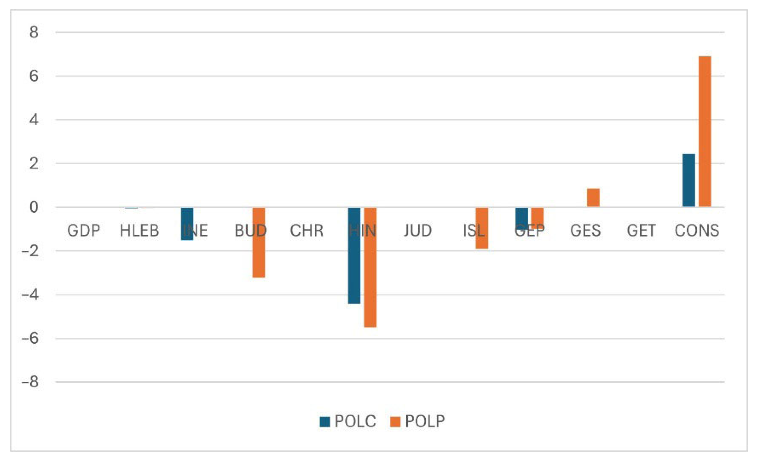
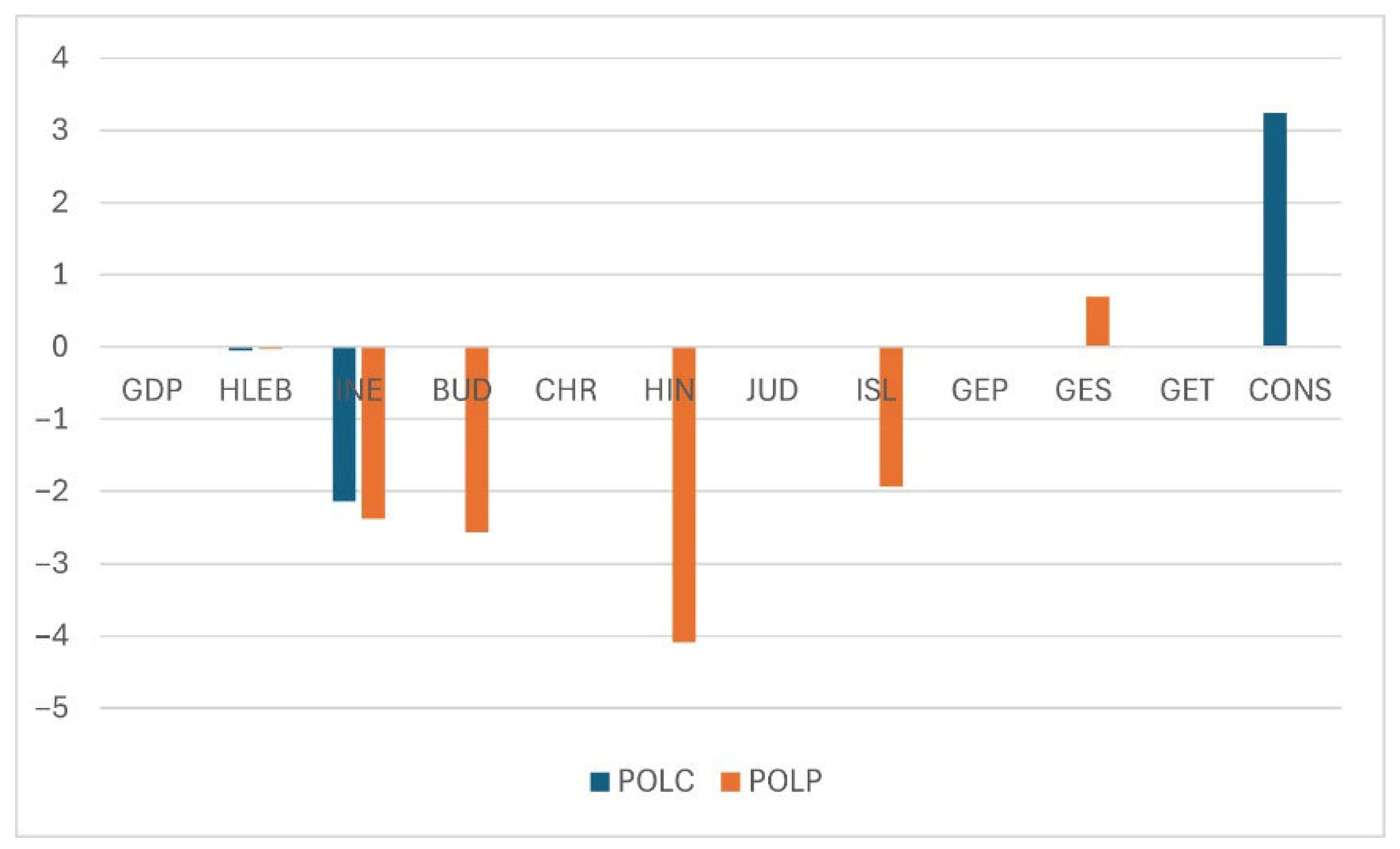
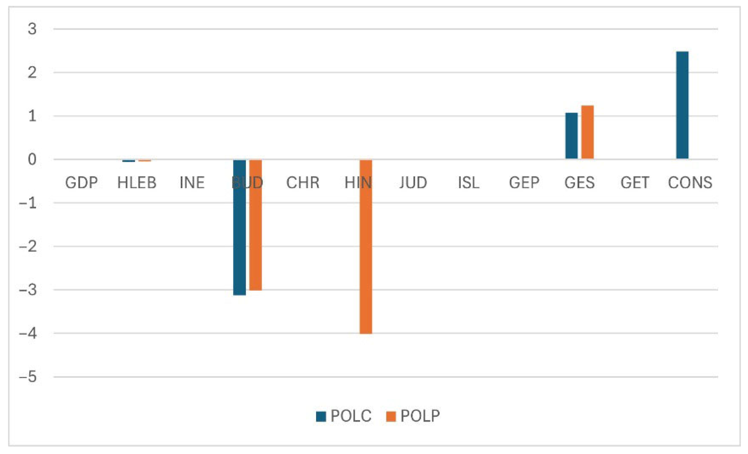
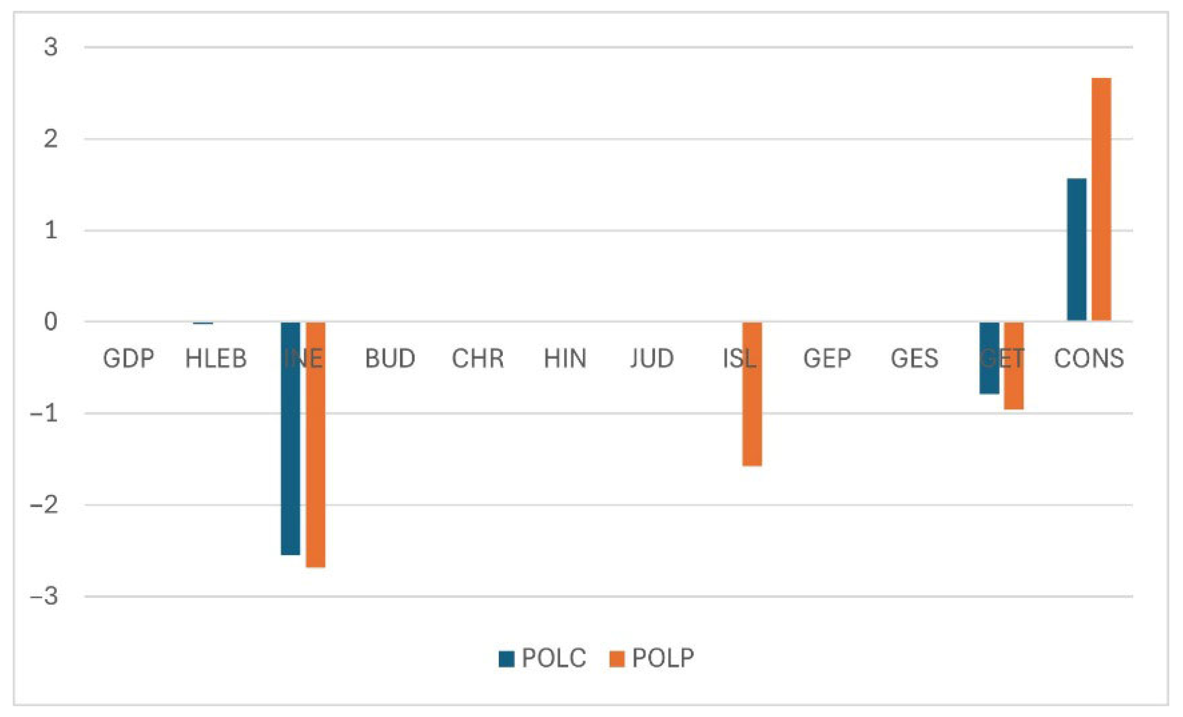
  • It did not use a dummy variable for hosting countries to reduce possible biases in medals in favour of them (i.e., athletes in hosting countries can have greater access to Olympic fields, courts, rivers, …). However, SFA estimations provided in Supplementary Materials S3 show that this dummy variable is positively significant in 5 out of 10 cases, particularly if GM and ∆G are the sport achievements under consideration (i.e., 2 out of 3 and 2 out of 2, respectively) and if POLP is the adopted sport policy (i.e., 3 out of 4). In other words, it is easier for hosting countries to obtain national pride by winning the GM and the gold match finals.
  • It did not use a time trend to avoid possible biases in favour of more recent sport achievements (i.e., the number of Olympic disciplines has increased over time). However, SFA estimations provided in Supplementary Materials S3 show that this time trend is negatively significant in 3 out of 10 cases, particularly if TM is the sport achievement under consideration (i.e., 2 out of 3). In other words, it is harder for original Olympic countries to win the same number of TM over time, due to the increasing number of Olympic countries.
Note that SFA does not require a balanced dataset like DEA. Consequently, adequate measures of additional features (e.g., gender inequality) could be used by SFA to show to what extent governmental objectives outside sport could affect sport achievements (e.g., women’s Olympic medals over men’s). Similarly, adequate measures of alternative contexts (e.g., collectivist vs. individualist cultures) could be used by SFA to show to what extent other socio-ethical contexts could affect sport achievements (e.g., total Olympic medals).
In summary, the present paper is a perfect example of Ethicametrics [68].

7. Conclusions

The purpose of this paper was to suggest a theoretical framework (GOAL 1) to summarise the empirical literature on the relationships between both ethics to and ethics through sport and both religious and secular ethics, and to suggest two interrelated theoretical models (GOAL 2) to empirically evaluate to what extent religious and secular ethics and sport policies affect achievements in sports, applying panel data analyses at a country level to Olympic Games as a case study of global ethics to and through sport.
The previous sections showed that my research succeeded topically. In particular, I detailed some expected results (i.e., I specified which religious ethics have larger negative impacts on sport achievements, and I specified which secular ethics have larger positive impacts on sport achievements). Moreover, I obtained many unexpected results (i.e., the positive impact of income level for GM larger than the positive impact of income level for TM, a negative impact of health status, and the negative impact of income inequality for GM smaller than the negative impact of income inequality for TM). Finally, I obtained some original results (i.e., the victory in the gold and bronze match finals as dependent on REL and SEC; decreasing returns for GM and constant returns to scale for TM).
In fact, my research was conducted in a much more methodological manner. In particular, I consistently applied PA and SFA obtaining comparable results (e.g., a positive impact of quantitative sport policy, a negative impact of health status). Moreover, I applied panel data analysis at the country level. Finally, I consistently applied SFA and DEA, obtaining comparable results (e.g., the crucial importance of quantitative sport policy, the crucial importance of health status).
Future developments could refer to doping practices in sports as the dependent variable (i.e., the avoidance of which is a governmental objective), to ethics of or ethics for sports (i.e., alternative ethical perspectives), or to educational protocols for sports as an independent variable (which is a governmental policy to be pursued).

Supplementary Materials

The supporting information SupMat123 can be downloaded at: https://www.mdpi.com/article/10.3390/stats8030067/s1.

Funding

This research received no external funding.

Institutional Review Board Statement

Not applicable.

Informed Consent Statement

Not applicable.

Data Availability Statement

Data available in a publicly accessible repository—The original data presented in the study are openly available in Olympic, World Religions and World Bank datasets at olympic.org, worldreligions.org and data.worldbank.org (accessed on 10 July 2025).

Conflicts of Interest

The authors declare no conflicts of interest.

Appendix A

Table A1. Checking goodness of fit for core estimations in PA and SFA. Abbreviations: PA = Poisson Analysis, SFA = Stochastic Frontier Analysis, GM = Gold Medals; TM = Total Medals; N = number of observations; LL = Log Likelihood; DF = Degree of Freedom; AIC = Akaike’s information criterion; BIC = Bayesian information criterion; AICc = corrected Akaike’s information criterion; CAIC = consistent Akaike’s information criterion.
NLLDFAICBICAICcCAIC
Table 4PAGM2056−871.633591761.2671811.9241761.3551820.924
Table 5PATM2182−2080.22794178.4544229.6464178.5374238.646
Table 6SFAGM600−860.8691121745.7381798.5011746.271810.501
Table 7SFATM850−1095.838122215.6762272.6192216.0492284.619
Table A2. Checking independence of hypotheses for core estimations in SFA.
P > zP List, Shaikh and XuP BonferroniP Holm
Table 6αPOLP0.7010.1630.3260.163
αPOLC0.0000.0900.0940.094
Table 7αPOLP0.501.0440.0890.044
αPOLC0.000.0020.0020.002
Table A3. Checking goodness of fit for detailed estimations in SFA. Abbreviations: GM = Gold Medals; TM = Total Medals; ∆G = winning the gold match final; ∆B = winning the bronze match final; POLC = a quantitative sport policy aimed at social cohesion; POLP = a qualitative sport policy aimed at national pride; BOTH = both sport policies; N = number of observations; LL = Log Likelihood; DF = Degree of Freedom; AIC = Akaike’s information criterion; BIC = Bayesian information criterion; AICc = corrected Akaike’s information criterion; CAIC = consistent Akaike’s information criterion.
NLLDFAICBICAICcCAIC
Table 6GMBOTH600−860.8691121745.7381798.5011746.271810.501
Table 7TMBOTH850−1095.838122215.6762272.6192216.0492284.619
Table 8GMPOLC600−856.8278171747.6561822.4031748.7071839.403
Table 9TMPOLC851−1093.036172220.0722300.7612220.8072317.761
Table 10∆GPOLC312−488.9894171011.9791075.611014.061092.61
Table 11∆BPOLC420−670.8647171375.7291444.4141377.2521461.414
Table 12GMPOLP600−902.743171839.4861914.2341840.5381931.234
Table 13TMPOLP850−1255.018172544.0362624.7052544.7722641.705
Table 14∆GPOLP312−492.8417171019.6831083.3141021.7651100.314
Table 15∆BPOLP419−675.6865171385.3731454.0171386.8991471.017

References

  1. Devine, J.W. Elements of excellence. J. Philos. Sport 2022, 49, 195–211. [Google Scholar] [CrossRef]
  2. Park, J.-H.; Choi, C.H.; Yoon, J.; Girginov, V. How should sports match fixing be classified? Cogent Soc. Sci. 2019, 5, 1–11. [Google Scholar] [CrossRef]
  3. Van Der Hoeven, S.; De Waegeneer, E.; Constandt, B.; Willem, A. Match-fixing: Moral challenges for those involved. Ethics Behav. 2020, 30, 425–443. [Google Scholar] [CrossRef]
  4. Moriconi, M.; Almeida, J.P. Portuguese Fight Against Match-Fixing: Which Policies and What Ethic? J. Glob. Sport Manag. 2019, 4, 79–96. [Google Scholar] [CrossRef]
  5. Csató, L. When neither team wants to win: A flaw of recent UEFA qualification rules. Int. J. Sports Sci. Coach. 2020, 15, 526–532. [Google Scholar] [CrossRef]
  6. Devine, J.W. O Captain! My Captain! leadership, virtue, and sport. J. Philos. Sport 2021, 48, 45–62. [Google Scholar] [CrossRef]
  7. Constandt, B.; Vertommen, T.; Cox, L.; Kavanagh, E.; Kumar, B.P.; Pankowiak, A.; Woessner, M. Quid interpersonal violence in the sport integrity literature? A scoping review. Sport Soc. 2024, 27, 162–180. [Google Scholar] [CrossRef]
  8. Lewandowski, J.D. Between rounds: The aesthetics and ethics of sixty seconds. J. Philos. Sport 2020, 47, 438–450. [Google Scholar] [CrossRef]
  9. Tabar, M.N.; Andam, R.; Bahrololoum, H.; Memari, Z.; Rezaei Pandari, A. Study of football social responsibility in Iran with Fuzzy cognitive mapping approach. Sport Soc. 2022, 25, 982–999. [Google Scholar] [CrossRef]
  10. Spruit, A.; Kavussanu, M.; Smit, T.; IJntema, M. The Relationship between Moral Climate of Sports and the Moral Behavior of Young Athletes: A Multilevel Meta-analysis. J. Youth Adolesc. 2019, 48, 228–242. [Google Scholar] [CrossRef] [PubMed]
  11. Ryba, T.V.; Schinke, R.J.; Quartiroli, A.; Wong, R.; Gill, D.L. ISSP position stand on cultural praxis in sport psychology: Reaffirming our commitments to the ethics of difference, cultural inclusion, and social justice. Int. J. Sport Exerc. Psychol. 2024, 22, 533–552. [Google Scholar] [CrossRef]
  12. Spowart, L. Navigating divorce, single-motherhood and long-distance triathlon: A visual-autoethnography. Sport Soc. 2024, 27, 1293–1313. [Google Scholar] [CrossRef]
  13. Ogunrinde, J.O. Toward a critical socioecological understanding of urban Black girls’ sport participation. Sport Educ. Soc. 2023, 28, 477–492. [Google Scholar] [CrossRef]
  14. Krieger, J.; Parks Pieper, L.; Ritchie, I. Sex, drugs and science: The IOC’s and IAAF’s attempts to control fairness in sport. Sport Soc. 2019, 22, 1555–1573. [Google Scholar] [CrossRef]
  15. Zakhem, A.; Mascio, M. Sporting Integrity, Coherence, and Being True to the Spirit of a Game. Sport Ethics Philos. 2019, 13, 227–236. [Google Scholar] [CrossRef]
  16. Hochstetler, D.; Linder, G.F.; Ball, J. Ethical discourses for and against doping in sport philosophy. J. Philos. Sport 2024, 51, 515–538. [Google Scholar] [CrossRef]
  17. Kirkwood, K.W. Of luck both epistemic and moral in questions of doping and non-doping. Ethics Prog. 2020, 11, 77–84. [Google Scholar] [CrossRef]
  18. Cooper, J. Testosterone: ‘the best discriminating factor’. Philosophies 2019, 4, 36. [Google Scholar] [CrossRef]
  19. McCalla, S. Sexism or fair play: Intersex women in competitive sports. Int. J. Appl. Philos. 2019, 33, 259–273. [Google Scholar] [CrossRef]
  20. Pike, J. Safety, fairness, and inclusion: Transgender athletes and the essence of Rugby. J. Philos. Sport 2021, 48, 155–168. [Google Scholar] [CrossRef]
  21. Hamilton, B.R.; Guppy, F.M.; Barrett, J.; Seal, L.; Pitsiladis, Y. Integrating transwomen athletes into elite competition: The case of elite archery and shooting. Eur. J. Sport Sci. 2021, 21, 1500–1509. [Google Scholar] [CrossRef]
  22. Shaw, A.L.; Williams, A.G.; Stebbings, G.K.; Chollier, M.; Harvey, A.; Heffernan, S.M. The perspective of current and retired world class, elite and national athletes on the inclusion and eligibility of transgender athletes in elite sport. J. Sports Sci. 2024, 42, 381–391. [Google Scholar] [CrossRef]
  23. Ordway, C.; Nichol, M.; Parry, D.; Tweedie, J.W. Human rights and inclusion policies for transgender women in elite sports: The case of Australia Rules Football (AFL). Sport Ethics Philos. 2023, 17, 1–23. [Google Scholar] [CrossRef]
  24. Frias, F.J.L.; Torres, C.R. The ethics of cloning horses in polo. Int. J. Appl. Philos. 2019, 33, 125–139. [Google Scholar] [CrossRef]
  25. Kulkarni, S.; McGannon, K.R.; Pegoraro, A. Expanding understanding of elite athlete parenthood in socio-cultural context: A meta-synthesis of qualitative media research findings on motherhood and sport. Sport Soc. 2024, 27, 1254–1273. [Google Scholar] [CrossRef]
  26. Twietmeyer, G.; Watson, N.J.; Parker, A. Sport, Christianity and Social Justice? Considering a Theological Foundation. Quest 2019, 71, 121–137. [Google Scholar] [CrossRef]
  27. Tak, M.; Kim, Y.J.; Rhind, D.J. Rights-based policies for role-bearing people: Are geo-cultural norms a hindrance to cultivating safer sport? Int. Rev. Sociol. Sport 2024, 60, 591–610. [Google Scholar] [CrossRef]
  28. Frias, F.J.L. Unnatural technology in a “natural” practice? Human nature and performance-enhancing technology in sport. Philosophies 2019, 4, 35. [Google Scholar] [CrossRef]
  29. De Waegeneer, E.; Constandt, B.; Van Der Hoeven, S.; Willem, A. Badminton Players’ Moral Intentions: A Factorial Survey Study into Personal and Contextual Determinants. Front. Psychol. 2019, 10, 2272. [Google Scholar] [CrossRef]
  30. Robertson, J.; Constandt, B. Moral disengagement and sport integrity: Identifying and mitigating integrity breaches in sport management. Eur. Sport Manag. Q. 2021, 21, 714–730. [Google Scholar] [CrossRef]
  31. Quartiroli, A.; Wagstaff, C. Continuing education in sport psychology: A survey of where we are and where we need to go. Int. J. Sport Exerc. Psychol. 2024, 1, 1–23. [Google Scholar] [CrossRef]
  32. Avner, Z.; Hall, E.T.; Potrac, P. Affect and emotions in sports work: A research agenda. Sport Soc. 2023, 26, 1161–1177. [Google Scholar] [CrossRef]
  33. Pankow, K.; Fraser, S.N.; Holt, N.L. A retrospective analysis of the development of psychological skills and characteristics among National Hockey League players. Int. J. Sport Exerc. Psychol. 2021, 19, 988–1004. [Google Scholar] [CrossRef]
  34. Aggerholm, K. Defiance in sport. J. Philos. Sport 2020, 47, 183–199. [Google Scholar] [CrossRef]
  35. Constantin, P.-N.; Stanescu, R.; Pelin, F.; Stoicescu, M.; Stanescu, M.; Barkoukis, V.; Vershuuren, P. How to Develop Moral Skills in Sport by Using the Corruption Heritage? Sustainability 2022, 14, 400. [Google Scholar] [CrossRef]
  36. Debognies, P.; Schaillée, H.; Haudenhuyse, R.; Theeboom, M. Personal development of disadvantaged youth through community sports: A theory-driven analysis of relational strategies. Sport Soc. 2019, 22, 897–918. [Google Scholar] [CrossRef]
  37. Uğraş, S.; Mergan, B.; Çelik, T.; Hidayat, Y.; Özman, C.; Üstün, Ü.D. The relationship between passion and athlete identity in sport: The mediating and moderating role of dedication. BMC Psychol. 2024, 12, 76. [Google Scholar] [CrossRef]
  38. Quartiroli, A.; Martin, D.R.; Hunter, H.; Wagstaff, C.R. A thematic-synthesis of self-care in sport psychology practitioners. Int. J. Sport Exerc. Psychol. 2023, 23, 1–25. [Google Scholar] [CrossRef]
  39. Park, S.; Lim, D. Applicability of Olympic Values in Sustainable Development. Sustainability 2022, 14, 5921. [Google Scholar] [CrossRef]
  40. Robertson, J.; Eime, R.; Westerbeek, H. Conceptualizing the contingent nature of social responsibility in sport. Res. Handb. Corp. Soc. Responsib. Sport 2025, 34–51. [Google Scholar] [CrossRef]
  41. Gunnell, K.E.; Belcourt, V.J.; Tomasone, J.R.; Weeks, L.C. Systematic review methods. Int. Rev. Sport Exerc. Psychol. 2022, 15, 5–29. [Google Scholar] [CrossRef]
  42. Yeh, C.-C.; Peng, H.-T.; Lin, W.-B. Achievement Prediction and Performance Assessment System for Nations in the Asian Games. Appl. Sci. 2024, 14, 789. [Google Scholar] [CrossRef]
  43. Ogwang, T.; Cho, D.I. Olympic rankings based on objective weighting schemes. J. Appl. Stat. 2021, 48, 573–582. [Google Scholar] [CrossRef] [PubMed]
  44. Reid, H.L. Olympic Philosophy: The Ideas and Ideals Behind the Ancient and Modern Olympic Games; Parnassos Press: Sioux City, IA, USA, 2020. [Google Scholar]
  45. Grix, J.; Gallant, D.; Brannagan, P.M.; Jones, C. Olympians’ Attitudes toward Olympic Values: A “Sporting” Life History Approach. J. Olymp. Stud. 2020, 1, 72–99. [Google Scholar] [CrossRef]
  46. Aggerholm, K. Sport humanism: Contours of a humanist theory of sport. J. Philos. Sport 2024, 52, 1–24. [Google Scholar] [CrossRef]
  47. Zurc, J. Ethical aspects of health and wellbeing of young elite athletes: Conceptual and normative issues. Synth. Philos. 2019, 34, 341–358. [Google Scholar] [CrossRef]
  48. Ribeiro, T.; Correia, A.; Biscaia, R.; Bason, T. Organizational Issues in Olympic Games: A Systematic Review. Event Manag. 2021, 25, 135–154. [Google Scholar] [CrossRef]
  49. Bakhtiyarova, S.; Murzakhmetov, Y.; Kashkynbai, K.M.; Kuderiyev, Z.K.; Sundetov, M. Olympic education as one of the priority areas of physical education and sports specialists. J. Phys. Educ. Sport 2020, 20, 273–279. [Google Scholar]
  50. Muñoz, J.; Solanellas, F.; Crespo, M.; Kohe, G.Z. Governance in regional sports organisations: An analysis of the Catalan sports federations. Cogent Soc. Sci. 2023, 9, 2209372. [Google Scholar] [CrossRef]
  51. Park, K.; Ok, G. The Legacy of Sports Nationalism in South Korean Sport. Int. J. Hist. Sport 2022, 39, 787–801. [Google Scholar] [CrossRef]
  52. Flegl, M.; Andrade, L.A. Measuring countries’ performance at the Summer Olympic Games in Rio 2016. Opsearch 2018, 55, 823–846. [Google Scholar] [CrossRef]
  53. Globan, T.; Rewilak, J. A new index to rank nations at the Summer Olympics. Manag. Sport Leis. 2024, 29, 1–19. [Google Scholar] [CrossRef]
  54. Loland, S. Classification in sport: A question of fairness. Eur. J. Sport Sci. 2021, 21, 1477–1484. [Google Scholar] [CrossRef] [PubMed]
  55. Meeuwsen, S.; Kreft, L. Sport and Politics in the Twenty-First Century. Sport Ethics Philos. 2023, 17, 342–355. [Google Scholar] [CrossRef]
  56. Han, X.; Zou, Y. Research on the group path of improving the efficiency of China’s public sports services based on DEA and fsQCA analysis. Sci. Rep. 2024, 14, 29482. [Google Scholar] [CrossRef] [PubMed]
  57. Kovács, K.; Oláh, Á.J.; Pusztai, G. The role of parental involvement in academic and sports achievement. Heliyon 2024, 10, e24290. [Google Scholar] [CrossRef] [PubMed]
  58. Sofyan, D.; Hafezad Abdullah, K.; Uriri Osiobe, E.; Indrayogi, I.; Mustafillah Rusdiyanto, R.; Gazali, N.; Touvan Juni Samodra, Y. Sport and religion: A mapping analytical research. Int. J. Public Health Sci. 2023, 12, 1302–1310. [Google Scholar] [CrossRef]
  59. Wan, K.-M.; Ng, K.-U.; Lin, T.-H. The Political Economy of Football: Democracy, Income Inequality, and Men’s National Football Performance. Soc. Indic. Res. 2020, 151, 981–1013. [Google Scholar] [CrossRef]
  60. Sitthiyot, T.; Holasut, K. A quantitative method for benchmarking fair income distribution. Heliyon 2022, 8, e10511. [Google Scholar] [CrossRef]
  61. Marinho, B.; Do Amaral, F.V.V.; Luz, L.G.O.; Guimarães, G.L.; Batista, L.A.; Chagas, D.V. Generic motor tests as tools to identify sports talent: A systematic review. Hum. Mov. 2024, 25, 53–63. [Google Scholar] [CrossRef]
  62. Güllich, A.; Barth, M. Effects of Early Talent Promotion on Junior and Senior Performance: A Systematic Review and Meta-Analysis. Sports Med. 2024, 54, 697–710. [Google Scholar] [CrossRef]
  63. Lozano, S.; Villa, G. Multi-objective centralized DEA approach to Tokyo 2020 Olympic Games. Ann. Oper. Res. 2023, 322, 879–919. [Google Scholar] [CrossRef]
  64. Herzer, D.; Strulik, H. Religiosity and income: A panel cointegration and causality analysis. Appl. Econ. 2017, 49, 2922–2938. [Google Scholar] [CrossRef]
  65. Podinovski, V.V. Direct estimation of marginal characteristics of nonparametric production frontiers in the presence of undesirable outputs. Eur. J. Oper. Res. 2019, 279, 258–276. [Google Scholar] [CrossRef]
  66. Aigner, L.; Asmild, M. Identifying the most important set of weights when modelling bad outputs with the weak disposability approach. Eur. J. Oper. Res. 2023, 310, 751–759. [Google Scholar] [CrossRef]
  67. Bačík, V. Olympic medalists of the modern summer Olympic games 1896–2016. J. Maps 2021, 17, 145–153. [Google Scholar] [CrossRef]
  68. Zagonari, F. Ethicametrics: A New Interdisciplinary Science. Stats 2025, 8, 50. [Google Scholar] [CrossRef]
Figure 1. Comparing significant impacts on GM provided in Table 8 and Table 12. Notes: CONS = constant, whereas acronyms of variables are summarized in Table 2.
Stats 08 00067 g001
Figure 2. Comparing significant impacts on TM provided in Table 9 and Table 13. Notes: CONS = constant, whereas acronyms of variables are summarized in Table 2.
Stats 08 00067 g002
Figure 3. Comparing significant impacts on ∆G provided in Table 10 and Table 14. Notes: CONS = constant, whereas acronyms of variables are summarized in Table 2.
Stats 08 00067 g003
Figure 4. Comparing significant impacts on ∆B provided in Table 11 and Table 15. Notes: CONS = constant, whereas acronyms of variables are summarized in Table 2.
Stats 08 00067 g004
Figure 5. Dummies from SFA applied to GM. Abbreviations: DEU = Germany, RUS = Russia, USA = United States of America.
Stats 08 00067 g005
Figure 6. Dummies from SFA applied to TM. Abbreviations: DEU = Germany, RUS = Russia, USA = United States of America.
Stats 08 00067 g006
Table 1. The theoretical framework and the expected impacts. Abbreviations: GM = gold medals, SM = Silver medals, BM = bronze medals, WM = wood medals, TM = total medals, μ = inefficiency score, θ = efficiency score, + = expected positive impact, − = expected negative impact, blank = no expected impacts, CM = country dummies, MO = Multi-Output. Notes: Social ethics = reward hard work, dedication and resilience; REL will be split into BUD, CHR, HIN, ISL, and JUD in additional estimations; SEC will be split into PRIMARY, SECONDARY, and TERTIARY in additional estimations; POL will be used as POLP for national pride and POLC for social cohesion.
Governmental
Objectives
(Output)
Indexes
(Input)
Variables
Methods
POLGDPHLEBINERELSEC
National
pride
Lexicographic
GM
+/−++/−+/−+Poisson Analysis
SFA
Social
cohesion
Sum
TM = GM + SM + BM
+/−++/−+/−+Poisson Analysis
SFA
Social
ethics
∆G = GM − SM,
∆B = BM − WM
+/−++/−+/−+SFA
National
efficiency
μ (inefficiency)
θ (efficiency)
θ (efficiency)
θ (efficiency)
+/−++/− SFA with CM
DEA Lexicographic
DEA Sum
MO DEA G, S, B
Table 2. Statistics of the variables used. Notes: all variables are per country and per Olympic event. Abbreviations: N = number of. Additional variables: ∆G = GM − SM, ∆S = SM − BM, ∆B = BM − WM, CONS = constant.
NameMeaningUnitMeanSDMAXMIN
GMGold MedalsN10.9010.751630
SMSilver MedalsN9.919.051100
BMBronze MedalsN9.708.85960
WMWood MedalsN9.417.35600
TMTotal MedalsN23.1514.383230
DIRconAthletes in direct games with contactN8.217.87560
INDAthletes in indirect gamesN20.5325.471610
DIRteaAthletes in direct games in teamsN37.9130.182740
DIRAthletes in direct gamesN34.9356.484620
POLPA qualitative policy aimed at national prideVariation’s coefficient of athletes across disciplines1.370.6020
POLCA quantitative policy aimed at social cohesionTotal number of athletes across disciplines61.5566.348561
GDPGross Domestic ProductCurrent Thousand USD15,89724,140208,835337
BUDBelievers in Buddhism%0.120.140.870.00
CHRBelievers in Christianity%0.570.390.990.00
HINBelievers in Hinduism%0.070.090.740.00
ISLBelievers in Islam%0.310.341.000.00
JUDBelievers in Judaism%0.030.060.740.00
RELSum of believers%0.860.351.010.00
SECSum of gross enrolment rates%0.730.321.270.00
GEPPrimary Gross Enrolment Rates%1.010.381.520.00
GESSecondary Gross Enrolment Rates%0.820.411.630.00
GETTertiary Gross Enrolment Rates%0.390.301.500.00
HLEBHealthy Life Expectancy at BirthYears62.8424.6976.9546.50
INEInequalityGini Index in [0, 1]0.380.160.650.24
POPPopulationMillion4115314230
Table 3. Summary of estimations performed. Abbreviations: * = for top 3 countries only.
GMTM∆G∆B
Poisson AnalysisBoth POL, REL, SECTable 4Table 5NONO
SFABoth POL, REL, SECTable 6Table 7NONO
POLC, specific REL and SECTable 8Table 9Table 10Table 11
POLP, specific REL and SECTable 12Table 13Table 14Table 15
Specific sports, REL and SECTable S1.1Table S1.2Table S1.3Table S1.4
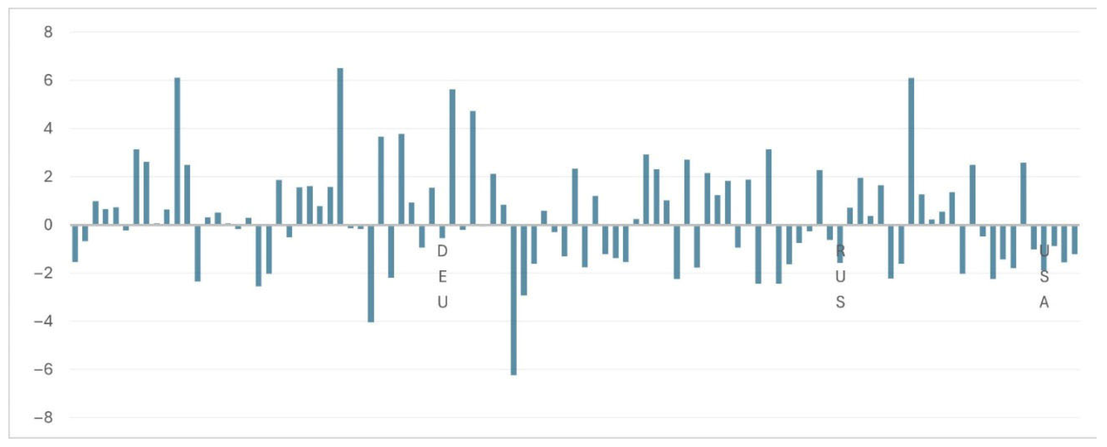
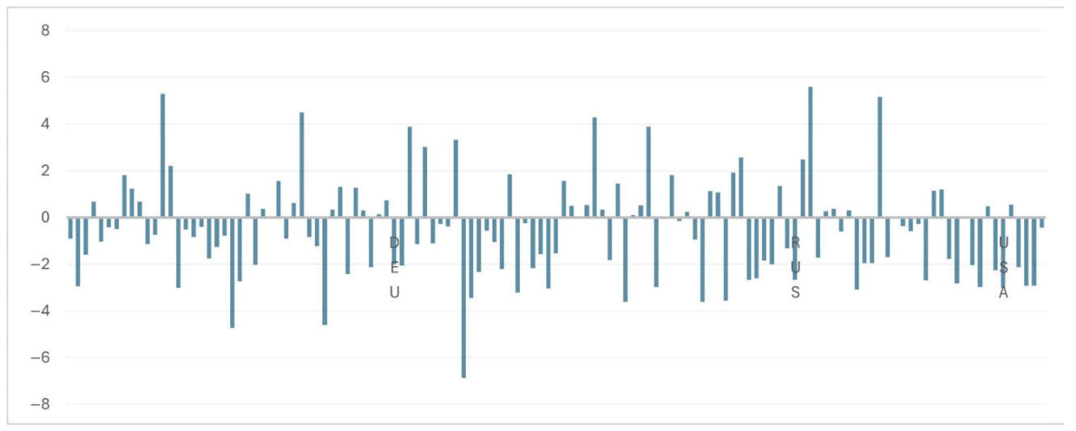
Both POL, REL, SEC
with country dummies
Table S2.1
Figure 1
Table S2.2
Figure 2
NONO
DEABoth POL, REL, SEC * Table 18 Table 18 NONO
Table 4. PA applied to GM. No. observations = 2056, No. groups = 206, Prob (random-effects model = pooled model) = 0. Bold = significant at 90%.
GMCoefficientStd. Err.zP > z[95% Conf.Interval]
POLP−1.0529730.2145596−4.910.000−1.473502−0.632444
POLC0.00601810.00061469.790.0000.00481350.0072227
GDP0.0045030.00413681.090.276−0.00360490.012611
HLEB−0.04793970.0135697−3.530.000−0.0745357−0.0213437
INE−2.8903460.845927−3.420.001−4.548332−1.232359
REL−0.89957670.9050115−0.990.320−2.6733670.8742134
SEC2.2901740.43080725.320.0001.44580730.134541
CONS1.7607980.47082353.740.0000.83800062.683595
Table 5. PA applied to TOTAL medals. No. observations = 2182, No. groups = 206, Prob (random-effects model = pooled model) = 0. Bold = significant at 90%.
TMCoefficientStd. Err.zP > z[95% Conf.Interval]
POLP−1.9274090.1185815−16.250.000−2.159824−1.694993
POLC0.00370320.000338310.950.0000.00304020.0043663
GDP0.0132010.00204386.460.0000.00919530.0172067
HLEB−0.0420490.0080627−5.220.000−0.0578517−0.0262463
INE1.5823270.59470532.660.0080.41672572.747928
REL−0.25166340.4606511−0.550.585−1.1545230.6511962
SEC−0.78667660.231724−3.390.001−1.240847−0.332506
CONS4.2289670.351683312.020.0003.539684.918253
Table 6. SFA applied to GM and both POL. No. observations = 600, No. groups = 100, significant μ (average inefficiency) = 2.248, non-significant η (increasing inefficiency) = 0.000, σu2 (similarity between countries) = 4.340, σv2 (similarity between countries over time) = 0.631. Bold = significant at 90%.
LnGMCoefficientStd. Err.zP > z[95% Conf.Interval]
LnPOLP−0.06318340.1647541−0.380.701−0.38609560.2597288
LnPOLC0.80359040.071525611.240.0000.66340280.943778
GDP0.00713880.00400261.780.074−0.00070610.0149838
HLEB−0.05952450.012079−4.930.000−0.0831989−0.03585
INE−1.627680.8402739−1.940.053−3.2745860.0192268
REL0.3090630.67551960.460.647−1.0149311.633057
SEC−0.42258080.5338317−0.790.429−1.4688720.6237101
CONS1.9366990.51758063.740.0000.92225982.951139
Table 7. SFA applied to TM and both POL. No. observations = 850, No. groups = 128, significant μ (average inefficiency) = 4.695, significant η (increasing inefficiency) = 0.001, σu2 (similarity between countries) = 3.249, σv2 (similarity between countries over time) = 0.453. Bold = significant at 90%.
LnTMCoefficientStd. Err.zP > z[95% Conf.Interval]
LnPOLP−0.07571330.1126301−0.670.501−0.29646430.1450377
LnPOLC1.0807570.050750821.300.0000.98128781.180227
GDP0.00202530.00305170.660.507−0.00395580.0080065
HLEB−0.04708240.0085301−5.520.000−0.063801−0.0303637
INE−2.1916150.6757723−3.240.001−3.516104−0.8671255
REL0.16706220.38777920.430.667−0.59297110.9270956
SEC−0.34477630.3543987−0.970.331−1.0393850.3498325
CONS3.4675911.3553192.560.0110.81121476.123968
Table 8. SFA applied to GM and POLC. No. observations = 600, No. groups = 100, significant μ (average inefficiency) = 3.327, non-significant η (increasing inefficiency) = −0.000, σu2 (similarity between countries) = 2.823, σv2 (similarity between countries over time) = 0.632. Bold = significant at 90%.
LnGMCoefficientStd. Err.zP > z[95% Conf.Interval]
LnPOLC0.79697840.066858111.920.0000.6659390.9280179
GDP0.00740250.00423571.750.081−0.00089920.0157042
HLEB−0.04220960.0124041−3.400.001−0.0665211−0.0178981
INE−1.5190870.8829199−1.720.085−3.2495780.2114044
BUD−2.3358971.467871−1.590.112−5.212870.5410772
CHR−0.2443770.5193302−0.470.638−1.2622460.7734915
HIN−4.4075072.399516−1.840.066−9.1104730.2954589
JUD−0.4894742.438828−0.200.841−5.269494.290542
ISL−0.46283660.6683368−0.690.489−1.7727530.8470795
GEP−1.0240380.5456254−1.880.061−2.0934450.0453677
GES0.50681590.36529171.390.165−0.20914271.222775
GET−0.33172270.3147018−1.050.292−0.94852690.2850816
CONS2.4549060.79451023.090.0020.8976954.012118
Table 9. SFA applied to TM and POLC. No. observations = 851, No. groups = 128, significant μ (average inefficiency) = 4.394, non-significant η (increasing inefficiency) = 0.001, σu2 (similarity between countries) = 2.871, σv2 (similarity between countries over time) = 0.458. Bold = significant at 90%.
LnTMCoefficientStd. Err.zP > z[95% Conf.Interval]
LnPOLC1.0768010.045959423.430.0000.98672231.16688
GDP0.0027120.00309840.880.381−0.00336080.0087848
HLEB−0.04781290.008295−5.760.000−0.0640708−0.0315551
INE−2.1372350.6913677−3.090.002−3.49229−0.7821788
BUD−1.8164151.292973−1.400.160−4.3505940.7177646
CHR0.4854660.37275091.300.193-.24511231.216044
HIN−2.4371351.696278−1.440.151−5.761780.8875094
JUD0.18674732.429090.080.939−4.5741824.947677
ISL−0.2766690.4429708−0.620.532−1.1448760.5915378
GEP−0.33696140.316855−1.060.288−0.95798580.284063
GES0.09436820.27125770.350.728−0.43728720.6260236
GET−0.06860110.2376173−0.290.773−0.53432260.3971203
CONS3.2469011.5419852.110.0350.22466646.269136
Table 10. SFA applied to ∆G medals and POLC. No. observations = 312, No. groups = 93, significant μ (average inefficiency) = 2.764, non-significant η (increasing inefficiency) = −0.003, σu2 (similarity between countries) = 2.095, σv2 (similarity between countries over time) = 0.751. Bold = significant at 90%.
Ln∆GCoefficientStd. Err.zP > z[95% Conf.Interval]
LnPOLC0.39169150.09645044.060.0000.20265230.5807307
GDP0.00877580.00597381.470.142−0.00293260.0204843
HLEB−0.04955880.0154762−3.200.001−0.0798917−0.0192259
INE−1.0593791.140695−0.930.353−3.29511.176342
BUD−3.1227781.588258−1.970.049−6.235705−0.0098499
CHR0.08391870.58164820.140.885−1.0560911.223928
HIN−3.6721022.354621−1.560.119−8.2870750.9428711
JUD−0.06423542.20858−0.030.977−4.3929724.264501
ISL−0.4347020.6512745−0.670.504−1.7111770.8417726
GEP−0.54529430.7453215−0.730.464−2.0060980.9155089
GES1.0831080.48867332.220.0270.12532552.04089
GET−0.12394010.5536306−0.220.823−1.2090360.961156
CONS2.4890421.1977962.080.0380.1414064.836679
Table 11. SFA applied to ∆B medals and POLC. No. observations = 420, No. groups = 103, non-significant μ (average inefficiency) = 0.423, significant η (increasing inefficiency) = −0.000, σu2 (similarity between countries) = 4.733, σv2 (similarity between countries over time) = 0.866. Bold = significant at 90%.
Ln∆BCoefficientStd. Err.zP > z[95% Conf.Interval]
LnPOLC0.41426820.09866164.200.0000.22089490.6076414
GDP0.01000380.0053071.890.059−0.00039770.0204053
HLEB−0.026280.0141699−1.850.064−0.05405260.0014926
INE−2.5522321.218396−2.090.036−4.940244−0.1642198
BUD−0.89128921.191349−0.750.454−3.2262891.443711
CHR0.30145650.5627050.540.592−0.80142511.404338
HIN−0.1900772.093201−0.090.928−4.2926753.912521
JUD−0.16410361.537227−0.110.915−3.1770142.848806
ISL−0.88469790.6109603−1.450.148−2.0821580.3127623
GEP−0.45983440.6704948−0.690.493−1.773980.8543112
GES0.10218340.50522790.200.840−0.8880451.092412
GET−0.78766960.4401333−1.790.074−1.6503150.0749758
CONS1.5667950.55196832.840.0050.48495722.648633
Table 12. SFA applied to GM and POLP. No. observations = 600, No. groups = 100, significant μ (average inefficiency) = 5.572, non-significant η (increasing inefficiency) = −0.002, σu2 (similarity between countries) = 1.841, σv2 (similarity between countries over time) = 0.802. Bold = significant at 90%.
LnGMCoefficientStd. Err.zP > z[95% Conf.Interval]
LnPOLP−0.84801620.1630012−5.200.000−1.167493−0.5285397
GDP0.01128220.00467332.410.0160.00212280.0204416
HLEB−0.02438530.0121951−2.000.046−0.0482871−0.0004834
INE−1.5215170.971031−1.570.117−3.4247030.3816687
BUD−3.2258541.320531−2.440.015−5.814048−0.6376606
CHR−0.64186750.5311708−1.210.227−1.6829430.3992082
HIN−5.4805611.982397−2.760.006−9.365989−1.595134
JUD−1.4248752.036209−0.700.484−5.415772.566021
ISL−1.9059650.6042405−3.150.002−3.090255−0.7216758
GEP−0.98293140.5885843−1.670.095−2.1365350.1706725
GES0.86477460.39819952.170.0300.08431791.645231
GET−0.33745330.3495964−0.970.334−1.022650.3477431
CONS6.905942.1311873.240.0012.7288911.08299
Table 13. SFA applied to TM and POLP. No. observations = 850, No. groups = 128, non-significant μ (average inefficiency) = 8.190, non-significant η (increasing inefficiency) = −0.000, σu2 (similarity between countries) = 1.872, σv2 (similarity between countries over time) = 0.766. Bold = significant at 90%.
LnTMCoefficientStd. Err.zP > z[95% Conf.Interval]
LnPOLP−1.1063230.1284515−8.610.000−1.358084−0.8545632
GDP0.00931050.00384252.420.0150.00177930.0168417
HLEB−0.02305140.0085382−2.700.007−0.0397859−0.0063169
INE−2.3785380.8423017−2.820.005−4.029419−0.7276569
BUD−2.5668341.129472−2.270.023−4.780558−0.3531098
CHR−0.06044620.4314735−0.140.889−0.90611870.7852263
HIN−4.0909671.557554−2.630.009−7.143717−1.038217
JUD−0.65648021.962348−0.330.738−4.5026123.189652
ISL−1.9276650.4552839−4.230.000−2.820005−1.035325
GEP−0.33612170.390846−0.860.390−1.1021660.4299224
GES0.69940610.33331052.100.0360.04612941.352683
GET−0.18631060.3111−0.600.549−0.79605540.4234341
CONS9.89644714.907190.660.507−19.321139.11399
Table 14. SFA applied to ∆G and POLP. No. observations = 312, No. groups = 93, non-significant μ (average inefficiency) = 10.539, non-significant η (increasing inefficiency) = −0.001, σu2 (similarity between countries) = 1.516, σv2 (similarity between countries over time) = 0.816. Bold = significant at 90%.
Ln∆GCoefficientStd. Err.zP > z[95% Conf.Interval]
LnPOLP−0.59117080.2476905−2.390.017−1.076635−0.1057063
GDP0.0115220.00575892.000.0450.00023480.0228092
HLEB−0.04307760.0151426−2.840.004−0.0727566−0.0133986
INE−1.1656421.1413−1.020.307−3.4025491.071265
BUD−3.0060291.405671−2.140.032−5.761094−0.2509643
CHR−0.04280120.5789178−0.070.941−1.1774591.091857
HIN−4.0121812.060582−1.950.052−8.0508490.026486
JUD−0.409271.969264−0.210.835−4.2689563.450416
ISL−0.9879210.635373−1.550.120−2.2332290.2573873
GEP−0.75730140.7528087−1.010.314−2.2327790.7181765
GES1.2401190.4879212.540.0110.28381112.196426
GET0.15787920.55966750.280.778−0.93904891.254807
CONS11.454727.7138351.480.138−3.66412226.57356
Table 15. SFA applied to ∆B and POLP. No. observations = 419, No. groups = 103, non-significant μ (average inefficiency) = 0.282, non-significant η (increasing inefficiency) = −0.001, σu2 (similarity between countries) = 4.078, σv2 (similarity between countries over time) = 0.949. Bold = significant at 90%.
Ln∆BCoefficientStd. Err.zP > z[95% Conf.Interval]
LnPOLP−0.44416020.2117808−2.100.036−0.8592429−0.0290774
GDP0.01302380.00553222.350.0190.0021810.0238666
HLEB−0.01700130.0139894−1.220.224−0.044420.0104173
INE−2.6832021.235406−2.170.030−5.104552−0.2618518
BUD−1.400821.189057−1.180.239−3.7313290.9296888
CHR0.09824080.57214480.170.864−1.0231421.219624
HIN−1.434162.08493−0.690.492−5.5205482.652228
JUD−0.40208861.435406−0.280.779−3.2154332.411256
ISL−10.5781770.5862269−2.690.007−2.727161−0.4291934
GEP−0.46847070.7045606−0.660.506−1.8493840.9124427
GES0.37863610.51964620.730.466−0.63985161.397124
GET−0.95863320.446888−2.150.032−1.834518−0.0827489
CONS2.6653010.50448865.280.0001.6765223.65408
Table 16. Marginal impacts on Olympic achievements. Abbreviations: GM = Gold Medals, TM = Total Medals, P = a statistically positive impact, PP = two statistically positive impacts, N = a statistically negative impact, NN = two statistically negative impacts, 0 = no statistically significant impact.
Table 8Table 9Table 12Table 13SumSumSumSum
GM and POLCTM and POLCGM and POLPTM and POLPGMTMPOLCPOLP
BUD00NNNN0NN
CHR00000000
HINN0NNNNNNNN
JUD00000000
ISL00NNNN0NN
GEPN0N0NN0NNN
GES00PPPP0PP
GET0000 00
POLP NNNN NN
POLCPP PPPP
GDPP0PPPPPPPP
HLEBNNNNNNNNNNNN
INENN0NNNNNNN
Table 17. Top 10 countries for alternative nation’s objectives. Notes: ° = 20 countries better ranked than Norway; * = 32 countries better ranked than Korea.
CouNamCouCodCouNumGOLDRankTOTALRank∆GOLDRank∆BRONZERank
United StatesUSA25211021245110.1520.085
Russian FederationRUS201463213882−0.0290.038
GermanyDEU874423125730.0530.066
ChinaCHN454044105140.035−0.0311
CanadaCAN37304587660.0440.029
AustraliaAUS12272610255−0.06100.182
FranceFRA8224877557−0.018−0.0110
NetherlandsNLD1722368641100.017−0.0913
United KingdomGBR2512149635110.0360.047
NorwayNOR18119810476130.170.103
KoreaKOR1251881154712−0.08110.251 *
JapanJPN119187126569−0.0812−0.0812
ItalyITA117170137028−0.09130.094
Table 18. DEA applied to GM, TM, and multi-medals for the top 3 countries (i.e., USA, RUS, and DEU).
GMθRankDummyRankPOLPPOLCGDPHLEBINERELSEC
USA0.5013−1.8830.1752.17212.0918.7310.0510.0850.114
RUS0.6592−1.5720.1834.8341.9988.3720.0520.1180.138
DEU0.8091−0.5410.0296.9551.2822.1310.0080.0330.024
Mean0.656 0.1294.6545.1246.4110.0370.0790.092
TMθRankDummyRankPOLPPOLCGDPHLEBINERELSEC
USA0.6893−3.0030.20913.25513.17012.5390.0750.1480.177
RUS0.7311−2.6720.2522.6094.68215.7660.0000.0920.231
DEU0.7212−2.0010.09921.3323.0137.8490.0320.1010.098
Mean0.713 0.18712.3986.95512.0510.0360.1140.168
MULTIθRank POLPPOLCGDPHLEBINERELSECGMSMBM
USA0.8203 0.10913.2578.2864.7970.0290.0650.0700.0180.0250.007
RUS0.8242 0.1162.1992.2068.2980.0550.1260.1400.0200.0410.019
DEU0.8551 0.0808.2843.7804.4180.0200.0600.0530.0320.0820.088
Mean 0.1017.9134.7575.8380.0350.0840.0880.0230.0490.038
Disclaimer/Publisher’s Note: The statements, opinions and data contained in all publications are solely those of the individual author(s) and contributor(s) and not of MDPI and/or the editor(s). MDPI and/or the editor(s) disclaim responsibility for any injury to people or property resulting from any ideas, methods, instructions or products referred to in the content.

