Machine Learning Ensemble Algorithms for Classification of Thyroid Nodules Through Proteomics: Extending the Method of Shapley Values from Binary to Multi-Class Tasks

Abstract

The need to improve medical diagnosis is of utmost importance in medical research, consisting of the optimization of accurate classification models able to assist clinical decisions. To minimize the errors that can be caused by using a single classifier, the voting ensemble technique can be used, combining the classification results of different classifiers to improve the final classification performance. This paper aims to compare the existing voting ensemble techniques with a new game-theory-derived approach based on Shapley values. We extended this method, originally developed for binary tasks, to the multi-class setting in order to capture complementary information provided by different classifiers. In heterogeneous clinical scenarios such as thyroid nodule diagnosis, where distinct models may be better suited to identify specific subtypes (e.g., benign, malignant, or inflammatory lesions), ensemble strategies capable of leveraging these strengths are particularly valuable. The motivating application focuses on the classification of thyroid cancer nodules whose cytopathological clinical diagnosis is typically characterized by a high number of false positive cases that may result in unnecessary thyroidectomy. We apply and compare the performance of seven individual classifiers, along with four ensemble voting techniques (including Shapley values), in a real-world study focused on classifying thyroid cancer nodules using proteomic features obtained through mass spectrometry. Our results indicate a slight improvement in the classification accuracy for ensemble systems compared to the performance of single classifiers. Although the Shapley value-based voting method remains comparable to the other voting methods, we envision this new ensemble approach could be effective in improving the performance of single classifiers in further applications, especially when complementary algorithms are considered in the ensemble. The application of these techniques can lead to the development of new tools to assist clinicians in diagnosing thyroid cancer using proteomic features derived from mass spectrometry.

1. Introduction

Thyroid nodules are exceedingly common; as much as half of all people are found to have at least one thyroid nodule by the age of 60. Fine needle aspiration biopsies (FNAs) are the first-line diagnostic tool for thyroid nodule evaluation. Fortunately, only 5 to 10% of thyroid nodules are found to be cancerous. However, how to distinguish between benign and malignant thyroid nodules is a crucial clinical challenge that has an impact on the appropriate management of patients, which indicates whether surgery or follow-up are necessary. Indeed, a significant percentage of these lesions (20–30%) is still “indeterminate for malignancy” at FNA, thus requiring diagnostic thyroidectomy, which often leads to a final histological diagnosis of benignity in around 80% of cases. Patients who undergo surgery to remove the thyroid gland need lifelong hormone replacement therapy, which is burdensome for the patient and leads to high healthcare costs for society. Different molecular tests pointing to abnormal molecular mechanisms of thyroid cancer, as genetic testing or gene-expression classifiers, have been proposed to improve the pre-operative risk assessment of malignancy on thyroid FNAs, but their costs still limit the implementation in routine clinical practice. Matrix-assisted laser desorption ionization mass spectrometry imaging (MALDI-MSI) represents a more conservative and less expensive tool to explore the spatial distribution of proteins directly in situ, integrating molecular and cytomorphological information. Preliminary results [1] suggest that the presence of different cell phenotypes are associated with specific mass spectra profiles. These results highlight the ability of proteomic MALDI-MSI analysis to generate specific molecular signatures representing different clinical entities.

The most widespread supervised machine learning and deep learning techniques, such as penalized regression, artificial neural networks, decision trees, and support vector machines, are often used for the prediction of prognosis or diagnosis on biological data. However, each classifier has its own strengths and weaknesses; consequently, choosing only one classifier for the analysis of complex data, such as mass spectrometry, could not be straightforward. The possibility to integrate many classifiers together can lead to an improvement in classification results because unrelated errors created by a single classifier can be avoided [2]. Two main voting systems exist to combine similar or conceptually different machine learning classifiers to predict the final class label [3]: 1. The final class label is the one that has been predicted most frequently by the classification models (majority voting). 2. The final class label is assessed by averaging the class probabilities of the different classifiers (averaging voting). These latter methods may also be improved by considering appropriate weights for each classifier, and in this weighted voting system, weights are assigned to the classifiers based on a specific criterion. The final prediction result is then obtained by averaging the weighted class probabilities. Usually, the weight of each classifier is chosen based on the performance, e.g., accuracy of the classifier in the training set, resulting in a higher weight for the classification model that performs better. It has been shown that the use of ensemble learners provides encouraging results in several studies where different classification approaches have been used [4,5]. In 2021, Benedek et al. [4] proposed the use of Shapley values (SVs) to weigh the different contributions of each classifier. This approach has been previously applied in different settings [5], such as in machine learning for feature selection, where SVs were used to measure feature importance: features were considered as players that cooperate to achieve high goodness of fit. Another machine learning domain for applying the SVs method is neural networks, pruning them to downsize overparameterized classifiers. This paper enhances the existing weighted voting ensemble learning technique and explores the new approach based on SVs to aid in the development of a diagnostic model for the prediction of thyroid cancer. To address the high heterogeneity in the diagnosis of thyroid cancer, also due to the possible misdiagnosis between cancer and Hashimoto disease, we extended the weighted voting system based on SVs from binary to multiple-class diagnostic problems. In such a heterogeneous diagnostic context, it is likely that different classifiers may excel at identifying specific patterns, for instance, one model might better distinguish malignant lesions, while another may be more sensitive to inflammatory or benign profiles. A voting method that incorporates the complementary contributions of individual classifiers can therefore offer improved reliability. For this reason, we aimed to extend the Shapley value ensemble approach, which is inherently designed to weigh each classifier’s marginal contribution, to multi-class problems involving complex clinical data.

The remainder of the paper is set up as follows. First, we illustrate the motivating clinical context. Subsequently, we introduce the concept of ensemble games, discuss SVs for the binary model, and present the extension suitable for multinomial classification. We evaluate the proposed algorithm, showing the application to the clinical study described above for both the binary and the multi-class classification tasks. Finally, we summarize our findings for each single machine learning algorithm and voting system and discuss the study limitations and future perspectives.

2. Materials and Methods

2.1. Patients

The cohort enrolled in this study is composed of 140 patients admitted to the ultrasound (US)-guided FNA at the ASST Monza (San Gerardo Hospital, University of Milano–Bicocca, Monza, Italy). Patients underwent a standard procedure of US-guided FNA that included a minimum of 2 needle passes per nodule. A morphological FNA diagnosis according to the 5-tiered SIAPEC/Bethesda reporting systems [6] was obtained by 2 expert cytopathologists. Patients with a non-malignant cytologic diagnosis underwent a 2-year follow-up monitoring to exclude the presence of echographic malignant features, while malignant or indeterminate cytological diagnosis underwent thyroidectomy. Patients were histologically classified according to the latest World Health Organization classification of endocrine tumours [7] as Hyperplastic (HP), Hashimoto Thyroiditis (HT), or Papillary Thyroid Carcinomas (PTC). We included 140 nodules in the study, corresponding to 70 HP, 54 PTC, and 16 HT. Patients with a clear diagnosis on cytologic examination were included in the training set, while indeterminate nodules with confirmed diagnosis in follow-up or histopathologic examinations contributed to the validation cohort.

Informed consent was obtained from patients included in the study. The study was approved by the Ethical Board of the ASST Monza (AIRC MFAG 2016, n.133/7-2-2017).

2.2. Mass Spectrometry

MALDI-MSI FNA thyroid needle washes were collected into a CytoLyt solution and prepared as previously described [8]. Then, they were transferred to indium tin oxide (ITO) slides directly and sent to MALDI-MSI examination. All the mass spectra were acquired in linear positive mode in the mass range of 3000 to 15,000 m/z, using 300 laser shots per spot, with a laser focus setting of 50 $\mathsf{\mu }$m and a pixel size of 50 × 50 $\mathsf{\mu }$m with an UltrafleXtreme mass spectrometer (Bruker Daltonics, Bremen, Germany). Data acquisition and visualization were performed using the Bruker software packages (flexControl $3.4$, flexImaging $5.0$). After MALDI-MSI analysis, the slides were stained with H&E and the cytological specimen was converted into digital by scanning the slide through the ScanScope CS digital scanner (Aperio, Park Center Dr., Vista, CA, USA), thus allowing the direct overlap and integration of cytomorphological and molecular information. Regions of interest (ROIs) containing specific pathological areas (i.e., benign and malignant thyrocytes, and lymphocites) were comprehensively annotated by the pathologist. All spectra from MALDI-MSI analysis were preprocessed as follows: baseline subtraction (median algorithm), smoothing (moving average method, half window width $=2.5$), normalization (Total Ion Current, TIC), peak alignment, and peak picking ($S/N\ge 6$) [1]. After having preprocessed mass spectrometry data, 1043 features were extracted and used to train all the classifiers. The high-dimensional nature of MSI data, which typically results in thousands of features, reflects the complex molecular content being captured. In this study, no feature selection was performed, as the focus was on evaluating ensemble learning strategies rather than optimizing the feature set. Data preprocessing was performed using the MALDIquant package (v.1.21) of the open-source R software (R Foundation for Statistical Computing, Vienna, Austria).

2.3. Statistical Methods

The statistical analysis of proteomic data was performed on the ROI average spectra generated by MALDI-MSI analysis in both the training and validation phases. For the training phase, the number of ROIs detected by pathologists from FNA biopsies of patients involved in the training cohort was 354 HP, 174 PTC, and 57 HT. For the validation cohort, 357 HP ROIs, 311 PTC ROIs, and 31 HT ROIs were available. The study includes analyses for both a binary classification problem (HP vs. PTC) and a multinomial classification problem (HP vs. HT vs. PTC). ROIs of HT nodules were included only in the multinomial model. To overcome bias in the results of the multinomial model due to the unbalanced number of ROIs of HT patients compared with PTC and HP, an equal number of ROIs were randomly selected, 50 ROIs for each class to construct the training cohort and 30 ROIs for each class constituting the validation phase. The selection was performed using the sample() function in the open-source R software, with a fixed random seed (set.seed(123)) to ensure reproducibility. Only ROIs previously confirmed by the pathologists as representative of either HP, HT or PTC phenotypes were considered for inclusion. This strategy allowed us to create a balanced dataset for the training and validation of the multinomial classification task, as previously explained, minimizing potential biases due to class imbalance.

2.3.1. Model Training and Hyperparameters

Among the standard classification models, seven were selected among those commonly adopted in the clinical literature relevant to our application domain, to form a diverse committee of expert models. These include the following: Extreme Gradient Boosting (XGB) [9], Random Forest (RF) [10], Multilayer Perceptron (MLP) [11], Support Vector Machine with linear (SVMlin) and polynomial (SVMpoly) kernels [12], K-Nearest Neighbors (KNNs) [13], and Gaussian Naive Bayes (NB) [14]. It is important to note that this list is not exhaustive of all algorithms proposed in the literature. Instead, we selected a representative and complementary set of models that are widely adopted in recent years, particularly in clinical and biomedical applications. Among them, Random Forest (RF) and Extreme Gradient Boosting (XGB) represent advanced ensemble-based evolutions of the basic decision tree (DT) [15], both based on aggregations of multiple decision trees. The set also includes neural models like the Multilayer Perceptron (MLP), margin-based classifiers such as Support Vector Machines (SVMs) with linear and polynomial kernels, instance-based learning methods like K-Nearest Neighbors (KNNs), and probabilistic approaches exemplified by Gaussian Naive Bayes (NB).

All classifiers were implemented using scikit-learn (v1.6.1) and XGBoost (v2.1.4) Python packages. Hyperparameters were selected based on literature references and refined via grid search on the training set. XGB was configured with eval_metric=’logloss’, using the default n_estimators=100, learning_rate=0.1, and max_depth=3. The option use_label_encoder=False was also set. RF used n_estimators=100 and criterion=’gini’, with unlimited tree depth (max_depth=None), and default bootstrapping. MLP consisted of a single hidden layer with 100 units, using ReLU activation and Adam solver. The maximum number of iterations was set to 1000, without early stopping, and the random state fixed to 42 for reproducibility. SVMs were trained with two different kernels. The linear version was configured with C=2, kernel=’linear’ and probability=True. The polynomial SVM used the same C=2, with kernel=’poly’, degree=3, and default settings for other parameters. KNN classification was performed with n_neighbors=5, using uniform weights, automatic algorithm selection, and Euclidean distance (p=2 in the Minkowski metric). NB was used with default settings, namely priors=None and var_smoothing=1E9.

2.3.2. Ensemble Construction

This diversity in modeling paradigms ensures a broad representation of learning strategies and supports robust ensemble construction. This selection of 7 algorithms was also crucial to enable the application of SV-based ensemble voting, a method designed to fairly quantify the predictive contribution of each classifier within an ensemble. SVs operate by evaluating the marginal contribution of a classifier across all possible subsets of the ensemble. Since the influence of each model depends on the composition of the subset to which it is added, this requires computing all possible permutations of classifiers. The resulting computational complexity grows factorially [4] with the number of models (n!), making it impractical to include a large number of classifiers. With 9 models, for example, 362,880 permutations (9!) would be needed, which is computationally prohibitive. By limiting the ensemble to seven classifiers, the number of required permutations is reduced to 5040 (7!), allowing the SVs computation to remain both feasible and meaningful.

Therefore, we applied the following ensemble voting schemes on these 7 performing classifiers:

• Simple majority voting system;
• Simple average voting system;
• Weighted average voting system by accuracy;
• Weighted average voting system by SVs.

Among these, the first three are typical combination methods [3], while the fourth is a novel class of cooperative ensemble methods based on game theory [4].

The study consisted of three consecutive stages.

• Construction of classifiers on the training set: in this stage, individual classifiers using the training set were constructed. Each of the 7 classifiers was trained to learn patterns and make predictions based on the given data.
• Evaluation of classifiers’ performance on a separate validation set: once the classifiers were constructed, their performances were evaluated using a separate validation set by the seven metrics (i.e., Accuracy, Specificity, Sensitivity, Negative Predictive Value (NPV), Positive Predictive Value (PPV) and their 95% Confidence Intervals (CIs)). Specifically, the ROIs classification was defined by the highest of the probabilities for the two classes (i.e., HP vs. PTC) and multiclass tasks (i.e., HP, HT, and PTC).
• Comparative evaluation of classifiers and combination rules: in this stage, a comparative evaluation of all the classifiers created and four different combination rules was performed. The four ensemble rules were evaluated both on all the seven standard classifiers (7cl) and on the best three classifiers (3cl) by Accuracy/SV.

All analyses were performed using the open-source R software v.4.4.2 and Python 3.7.12.

2.3.3. Voting Based on Shapley Values (SVs) for Binary Classification

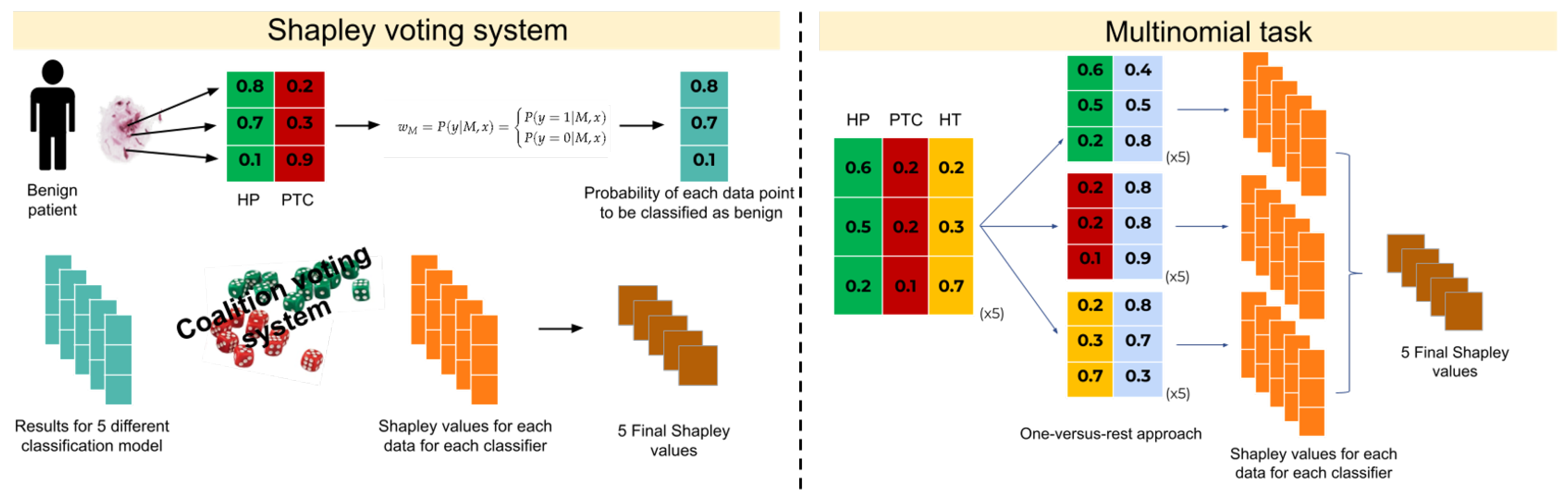
We define each of the m classifiers as a player of a game. In an ensemble game, players cooperate to classify every single unit of the cohort of size n (in our study, each unit is an ROI annotated by pathologists on the morphological FNA biopsy). Players vote to make an aggregated decision of the ensemble as follows:

• Assuming that the true label $y_i$ of each unit $x_i(i=1,\dots ,n)$ was known, for each binary classifier $M_j(j=1,\dots ,m)$, the probability of having a positive or negative classification is given by (1).

  $$w_{i_{M_j}}=P\left(y_i\right|M_j,x_i)=\left\{\begin{array}{c}P(y_i=1|M_j,x_i)\hfill \\ P(y_i=0|M_j,x_i)\hfill \end{array}\right.$$

  (1)
  These weights represent the confidence of each classifier to correctly classifying a single unit.
• For each possible subset of classifiers $S_k=\{M_1,\dots ,M_{m_{Sk}}\}$ where $m_{Sk}$ is the number of classifiers in the subset $S_k(k=1,\dots ,K)$ and K the total number of subsets, the average of the weights obtained by (1) is calculated in (2).

  $$w_i\left(S_k\right)={\displaystyle \frac{1}{m_{Sk}}}\sum _{M\in Sk}{w}_{i_{M_j}}$$

  (2)
• The outcome assigned to each unit depends on the value of $w_i\left(S_k\right)$. If its value is greater than a certain value between 0 and 1, i.e., 0.5, the class is equal to 1; otherwise, it is equal to 0. We define in (3) the payoff function of the game $f_i:2^m\to \{0,1\}$ as:

  $$f_i\left(S_k\right)=\left\{\begin{array}{c}1if{w}_i\left(S_k\right)>\gamma \hfill \\ 0otherwise.\hfill \end{array}\right.$$

  (3)
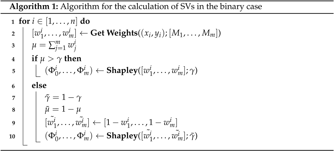
• Given the weights in (1), the next step is to calculate the SVs through the shapley Python library [4], here reported in the following Algorithm 1. In this equation, a SV for the unit i based on the m classifiers is calculated. For simplicity, we report the general formula in (4), where A is a player (in our case one of m classifiers), $\left|S\right|!$ considers the number of combinations before A in the possible subset of classifiers, $\left(\right|K|-|S|-1)!$ refers to the number of combinations of classifiers after A, and $\left|K\right|!$ is the number of total combinations. This is multiplied by the marginal contribution of player A.

  $${\mathsf{\Phi }}_A(S,f)=\sum _{S\subseteq KA}{\displaystyle \frac{\left|S\right|!\left(\right|K|-|S|-1)!}{\left|K\right|!}}[f(S\cup A)-f\left(S\right)]$$

  (4)
  For each unit, the sum of the m SVs is equal to one. The SV represents a model’s contribution to correctly classifying the unit, "ranking" the classifiers with different weights from the most to the least accurate.
• For each classifier, the mean of the SVs of the n units was calculated, leading to one weight for each binary classifier, called the m final SVs.

Algorithm 1: Algorithm for the calculation of SVs in the binary case

2.3.4. Extension of Voting Based on Shapley Values (SVs) for Multi-Class Tasks

In the case of the multinomial classification issue, the idea was to reduce the multi-class problem into a binary case using a one-versus-rest approach. The SVs were trained for each classifier per class (P), then the mean of the P final SVs within each classifier were returned obtaining the final m SVs (see Algorithm 2).

Algorithm 2: Extension of the algorithm for the calculation of SVs in the multiclass case

//  Extract positive probabilities for each class 1  class0 = first column of the three-columns array of probs 2  class1 = second column of the three-columns array of probs 3  class2 = third column of the three-columns array of probs //  Calculate the negative probabilities for each class 4  versus-class0 = 1 - class0 5  versus-class1 = 1 - class1 6  versus-class2 = 1 - class2 //  Obtain the two-columns array for each class 7  class0-vs-all = [class0, versus-class0] 8  class1-vs-all = [class1, versus-class1] 9  class2-vs-all = [class0, versus-class2]

This strategy involves training the SVs of each classifier per class, looking at the probabilities of each class vs. the sum of probabilities of all other classes (considered as a unique class). With the one-versus-rest approach, the workflow previously described was applied to each class, resulting in $P*m$SVs, with P the number of classes and m the number of classifiers. The mean of the P final SVs within the classifier returns one value for each, and consequently the final m SVs. An exemplification overview of the SVs system is reported in Figure 1.

3. Results

We report here the results of the seven classifiers (i.e., XGB, RF, MLP, SVMlin, SVMpoly, KNN, NB) and the four voting systems (i.e., majority voting, mean voting, weighted mean voting with weights based on the classifiers’ accuracy estimated in the training set, and the novel and previously described method based on SVs with weights based on the classifiers’ SVs estimated in the training set) applied to the two- and three-class classification problem in the motivating clinical context of thyroid cancer.

3.1. Two Classes

For the two-class problem, we used a validation set of 668 ROIs: 357 HP and 311 PTC. The distribution of the ROI specific predicted probabilities of being in the two classes are reported in Appendix A Figure A1 for each classifier and voting system. The graph is divided into two panels that distinguish samples with HP as the pathologist’s classification (top panel) and those with PTC labels (bottom panel). The predicted probabilities of being HP were very high and thus consistent with the pathologist HP classification in almost all models, with roughly 75% of the ROI probabilities above 0.70. The ability of the different models to predict PTC shows heterogeneity in the response, and median predicted probabilities of being PTC are between 0.60 and 0.75 in the majority of models.

The performances of the binary classification in terms of accuracy are reported in

Table 1. Accuracy (with 95% confidence interval) of single classifiers and voting methods for the two-class classification problem (HP vs. PTC) in the validation set. Voting methods are based on the seven standard classifiers (7cl) and on the three best classifiers among the seven ones (3cl).

	Method	Accuracy	95% CI
Single Classifier	XGB	0.71	(0.68–0.75)
	RF	0.69	(0.65–0.73)
	MLP	0.75	(0.72–0.78)
	SVMlin	0.75	(0.72–0.78)
	SVMpoly	0.66	(0.63–0.70)
	KNN	0.71	(0.68–0.75)
	NB	0.76	(0.72–0.79)
Voting systems	Majority.vot.7cl	0.75	(0.72–0.78)
	Majority.vot.3cl	0.76	(0.72–0.79)
	Mean.vot.7cl	0.76	(0.73–0.80)
	Mean.vot.3cl	0.78	(0.74–0.81)
	Weighted.mean.acc.7cl	0.76	(0.72–0.79)
	Weighted.mean.acc.3cl	0.78	(0.74–0.81)
	Shapley.7cl	0.76	(0.72–0.79)
	Shapley.3cl	0.78	(0.74–0.81)

and Appendix A 

Table A1. Performance metrics (with 95% confidence interval) of single classifiers and voting methods for the two-class classification problem (HP and PTC) in the validation set. Voting methods are based on the seven standard classifiers (7cl) and on the three best classifiers among the seven (3cl).

Method	Specificity	Sensitivity	NPV	PPV
XGB	0.89 (0.85–0.92)	0.51 (0.45–0.57)	0.68 (0.63–0.72)	0.80 (0.74–0.85)
RF	0.64 (0.59–0.69)	0.75 (0.69–0.79)	0.74 (0.69–0.79)	0.64 (0.59–0.69)
MLP	0.91 (0.88–0.94)	0.57 (0.51–0.62)	0.71 (0.66–0.75)	0.85 (0.79–0.90)
SVMlin	0.77 (0.73–0.82)	0.72 (0.67–0.77)	0.76 (0.72–0.81)	0.74 (0.68–0.78)
SVMpoly	0.93 (0.90–0.95)	0.36 (0.30–0.41)	0.62 (0.58–0.67)	0.82 (0.74–0.88)
KNN	0.87 (0.83–0.91)	0.53 (0.47–0.58)	0.68 (0.63–0.72)	0.78 (0.72–0.84)
NB	0.76 (0.72–0.81)	0.75 (0.70–0.80)	0.78 (0.73–0.82)	0.74 (0.68–0.78)
Majority.vot.7cl	0.90 (0.86–0.93)	0.59 (0.53–0.64)	0.71 (0.67–0.75)	0.83 (0.77–0.88)
Majority.vot.3cl	0.82 (0.78–0.86)	0.68 (0.63–0.73)	0.75 (0.70–0.79)	0.77 (0.71–0.82)
Mean.vot.7cl	0.89 (0.85–0.92)	0.62 (0.57–0.68)	0.73 (0.69–0.77)	0.83 (0.77–0.87)
Mean.vot.3cl	0.82 (0.77–0.86)	0.73 (0.67–0.78)	0.77 (0.73–0.82)	0.78 (0.72–0.82)
Weighted.mean.acc.7cl	0.88 (0.84–0.91)	0.62 (0.57–0.68)	0.73 (0.68–0.77)	0.82 (0.76–0.86)
Weighted.mean.acc.3cl	0.82 (0.77–0.86)	0.73 (0.67–0.78)	0.77 (0.73–0.82)	0.78 (0.72–0.82)
Shapley.7cl	0.88 (0.84–0.91)	0.62 (0.57–0.68)	0.73 (0.68–0.77)	0.82 (0.76–0.86)
Shapley.3cl	0.82 (0.77–0.86)	0.73 (0.67–0.78)	0.77 (0.73–0.82)	0.78 (0.72–0.82)

. The best-performing methods are MLP, SVMlin, and NB, each achieving an accuracy of 75%. Although they reach the same overall accuracy, these classifiers exhibit contrasting behaviors in distinguishing between benign and malignant diagnoses (Table 1). MLP demonstrates a stronger ability to identify benign lesions, with a specificity of 91%, whereas NB is more effective in detecting malignant characteristics, achieving a sensitivity of 75%. Notably, SVMpoly attains the highest specificity among all models (93%), highlighting its strength in recognizing benign cases. On the other hand, RF matches NB in terms of sensitivity (75%), making it particularly suitable for identifying malignant lesions.

The overall poorest performance in sensitivity, however, was recorded by SVMpoly, which scored only 36% despite its high specificity. This suggests that SVMpoly is biased towards correctly classifying benign lesions, at the expense of misclassifying malignant ones (Appendix A Table A1).

Regarding the ensemble voting methods, all configurations yielded similar accuracies, ranging between 75% and 78%. As expected, ensemble systems based on the top three classifiers outperformed those including all seven, with the best results achieved by both simple and weighted average voting, as well as SV-based voting, each applied to the top three classifiers, reaching an accuracy of 78% (Appendix A Table A1). Interestingly, the highest specificity was achieved exclusively by the majority voting system involving all seven classifiers.

We also reported in Appendix A 

Table A2. Accuracy and SVs for the two-class classification problem (HP and PTC) in the training set.

	XGB	RF	MLP	SVMlin	SVMpoly	KNN	NB
Accuracy	100%	100%	99.2%	89.8%	93.8%	98.7%	100%
SVs	0.148	0.148	0.146	0.129	0.137	0.145	0.147

the accuracy and the SVs of the single classifiers on the training set. Notably, the rating of the single classifiers are the same based on the two metrics; this leads to equal results in the classification performances for the seven-classifiers and three-classifiers voting systems.

3.2. Three Classes

For the three-class problem, we used a reduced validation set to overcome bias due to the unbalanced number of ROIs of HT patients compared with PTC and HP. The predicted probabilities for the three classes are reported in Appendix A Figure A2. In general, the ensemble method showed good performance in the identification of HP and PTC ROIs compared to single classifiers that are more affected by errors. In contrast, the HT class resulted in a higher rate of incorrect final classifications, sharing similar characteristics to both the malignant and benign nodules. The pathogenetic prognostic relationship between HT and cancer is debated too; areas of cytologic atypia of the follicular epithelium in HT can be so prominent that they are mistaken for PTC [1,16,17].

Table 2. Accuracy (with 95% confidence interval) of single classifiers and voting methods for the three-class classification problem (HP, HT and PTC) in the validation set. Voting methods are based on the seven standard classifiers (7cl) and on the three best classifiers of the seven (3cl).

	Method	Accuracy	95% CI
Single Classifier	XGB	0.40	(0.30–0.51)
	RF	0.49	(0.38–0.60)
	MLP	0.33	(0.24–0.44)
	SVMlin	0.33	(0.24–0.44)
	SVMpoly	0.37	(0.27–0.47)
	KNN	0.44	(0.34–0.55)
	NB	0.40	(0.30–0.51)
Voting systems	Majority.vot.7cl	0.51	(0.40–0.62)
	Majority.vot.3cl	0.48	(0.37–0.59)
	Mean.vot.7cl	0.43	(0.33–0.54)
	Mean.vot.3cl	0.49	(0.38–0.60)
	Weighted.mean.acc.7cl	0.42	(0.32–0.53)
	Weighted.mean.acc.3cl	0.48	(0.37–0.59)
	Shapley.7cl	0.42	(0.32–0.53)
	Shapley.3cl	0.48	(0.37–0.59)

shows the summary results of the three-class classification task (HP, HT, and PTC) in terms of accuracy. To provide a more comprehensive description of the performance of the methods considered, we also made available the other performance metrics, considering a one-vs-others perspective, which are reported in Appendix A (

Table A3. Performance metrics (with 95% confidence interval) of single classifiers and voting methods for the three-class classification problem (HP vs. HT and PTC) in the validation set. Voting methods are based on the seven standard classifiers (7cl) and on the three best classifiers among the seven (3cl).

Method	Accuracy	Specificity	Sensitivity	NPV	PPV
XGB	0.68 (0.57–0.77)	0.60 (0.41–0.77)	0.72 (0.59–0.83)	0.51 (0.34–0.69)	0.78 (0.65–0.88)
RF	0.76 (0.65–0.84)	0.83 (0.65–0.94)	0.72 (0.59–0.83)	0.60 (0.43–0.74)	0.90 (0.77–0.97)
MLP	1.00 (0.88–1.00)	1.00 (0.88–1.00)	0.50 (0.00–1.00)	1.00 (0.88–1.00)	0.50 (0.00–1.00)
SVMlin	1.00 (0.88–1.00)	1.00 (0.88–1.00)	0.50 (0.00–1.00)	1.00 (0.88–1.00)	0.50 (0.00–1.00)
SVMpoly	0.71 (0.61–0.80)	0.23 (0.10–0.42)	0.95 (0.86–0.99)	0.70 (0.35–0.93)	0.71 (0.60–0.81)
KNN	0.71 (0.61–0.80)	0.73 (0.54–0.88)	0.70 (0.57–0.81)	0.55 (0.38–0.71)	0.84 (0.71–0.93)
NB	0.68 (0.57–0.77)	0.33 (0.17–0.53)	0.85 (0.73–0.93)	0.53 (0.29–0.76)	0.72 (0.60–0.82)
Majority.vot.7cl	0.79 (0.69–0.87)	0.87 (0.69–0.96)	0.75 (0.62–0.85)	0.63 (0.47–0.78)	0.92 (0.80–0.98)
Majority.vot.3cl	0.74 (0.64–0.83)	0.73 (0.54–0.88)	0.75 (0.62–0.85)	0.59 (0.42–0.75)	0.85 (0.72–0.93)
Mean.vot.7cl	0.71 (0.61–0.80)	0.60 (0.41–0.77)	0.77 (0.64–0.87)	0.56 (0.38–0.74)	0.79 (0.67–0.89)
Mean.vot.3cl	0.76 (0.65–0.84)	0.60 (0.41–0.77)	0.83 (0.71–0.92)	0.64 (0.44–0.81)	0.81 (0.69–0.90)
Weighted.mean.acc.7cl	0.71 (0.61–0.80)	0.60 (0.41–0.77)	0.77 (0.64–0.87)	0.56 (0.38–0.74)	0.79 (0.67–0.89)
Weighted.mean.acc.3cl	0.74 (0.64–0.83)	0.60 (0.41–0.77)	0.82 (0.70–0.90)	0.62 (0.42–0.79)	0.80 (0.68–0.89)
Shapley.7cl	0.71 (0.61–0.80)	0.60 (0.41–0.77)	0.77 (0.64–0.87)	0.56 (0.38–0.74)	0.79 (0.67–0.89)
Shapley.3cl	0.74 (0.64–0.83)	0.60 (0.41–0.77)	0.82 (0.70–0.90)	0.62 (0.42–0.79)	0.80 (0.68–0.89)

,

Table A4. Performance metrics (with 95% confidence interval) of single classifiers and voting methods for the three-class classification problem (HT vs. HP and PTC) in the validation set. Voting methods are based on the seven standard classifiers (7cl) and on the three best classifiers among the seven (3cl).

Method	Accuracy	Specificity	Sensitivity	NPV	PPV
XGB	0.54 (0.44–0.65)	0.17 (0.06–0.35)	0.73 (0.60–0.84)	0.24 (0.08–0.47)	0.64 (0.51–0.75)
RF	0.64 (0.54–0.74)	0.03 (0.00–0.17)	0.95 (0.86–0.99)	0.25 (0.01–0.81)	0.66 (0.55–0.76)
MLP	0.50 (0.37–0.63)	0.00 (0.00–0.12)	1.00 (0.88–1.00)	0.50 (0.00–1.00)	0.50 (0.37–0.63)
SVMlin	0.50 (0.37–0.63)	0.00 (0.00–0.12)	1.00 (0.88–1.00)	0.50 (0.00–1.00)	0.50 (0.37–0.63)
SVMpoly	0.61 (0.50–0.71)	0.00 (0.00–0.12)	0.92 (0.82–0.97)	0.00 (0.00–0.52)	0.65 (0.54–0.75)
KNN	0.60 (0.49–0.70)	0.03 (0.00–0.17)	0.88 (0.77–0.95)	0.12 (0.00–0.53)	0.65 (0.53–0.75)
NB	0.50 (0.39–0.61)	0.27 (0.12–0.46)	0.62 (0.48–0.74)	0.26 (0.12–0.45)	0.63 (0.49–0.75)
Majority.vot.7cl	0.64 (0.54–0.74)	0.00 (0.00–0.12)	0.97 (0.88–1.00)	0.00 (0.00–0.84)	0.66 (0.55–0.76)
Majority.vot.3cl	0.60 (0.49–0.70)	0.07 (0.01–0.22)	0.87 (0.75–0.94)	0.20 (0.03–0.56)	0.65 (0.54–0.75)
Mean.vot.7cl	0.57 (0.46–0.67)	0.07 (0.01–0.22)	0.82 (0.70–0.90)	0.15 (0.02–0.45)	0.64 (0.52–0.74)
Mean.vot.3cl	0.59 (0.48–0.69)	0.17 (0.06–0.35)	0.80 (0.68–0.89)	0.29 (0.10–0.56)	0.66 (0.54–0.76)
Weighted.mean.acc.7cl	0.56 (0.45–0.66)	0.07 (0.01–0.22)	0.80 (0.68–0.89)	0.14 (0.02–0.43)	0.63 (0.51–0.74)
Weighted.mean.acc.3cl	0.59 (0.48–0.69)	0.17 (0.06–0.35)	0.80 (0.68–0.89)	0.29 (0.10–0.56)	0.66 (0.54–0.76)
Shapley.7cl	0.56 (0.45–0.66)	0.07 (0.01–0.22)	0.80 (0.68–0.89)	0.14 (0.02–0.43)l	0.63 (0.51–0.74)
Shapley.3cl	0.59 (0.48–0.69)	0.17 (0.06–0.35)	0.80 (0.68–0.89)	0.29 (0.10–0.56)	0.66 (0.54–0.76)

and

Table A5. Performance metrics (with 95% confidence interval) of single classifiers and voting methods for the three-class classification problem (PTC vs. HP and HT) in the validation set. Voting methods are based on the seven standard classifiers (7cl) and on the three best classifiers among the seven (3cl).

Method	Accuracy	Specificity	Sensitivity	NPV	PPV
XGB	0.58 (0.47–0.68)	0.43 (0.25–0.63)	0.65 (0.52–0.77)	0.38 (0.22–0.56)	0.70 (0.56–0.81)
RF	0.58 (0.47–0.68)	0.60 (0.41–0.77)	0.57 (0.43–0.69)	0.41 (0.26–0.57)	0.74 (0.59–0.86)
MLP	0.50 (0.37–0.63)	0.00 (0.00–0.12)	1.00 (0.88–1.00)	0.50 (0.00–1.00)	0.50 (0.37–0.63)
SVMlin	0.50 (0.37–0.63)	0.00 (0.00–0.12)	1.00 (0.88–1.00)	0.50 (0.00–1.00)	0.50 (0.37–0.63)
SVMpoly	0.41 (0.31–0.52)	0.87 (0.69–0.96)	0.18 (0.10–0.30)	0.35 (0.24–0.47)	0.73 (0.45–0.92)
KNN	0.58 (0.47–0.68)	0.57 (0.37–0.75)	0.58 (0.45–0.71)	0.40 (0.26–0.57)	0.73 (0.58–0.85)
NB	0.62 (0.51–0.72)	0.60 (0.41–0.77)	0.63 (0.50–0.75)	0.45 (0.29–0.62)	0.76 (0.62–0.87)
Majority.vot.7cl	0.59 (0.48–0.69)	0.67 (0.47–0.83)	0.55 (0.42–0.68)	0.43 (0.28–0.58)	0.77 (0.61–0.88)
Majority.vot.3cl	0.61 (0.50–0.71)	0.63 (0.44–0.80)	0.60 (0.47–0.72)	0.44 (0.29–0.60)	0.77 (0.62–0.88)
Mean.vot.7cl	0.59 (0.48–0.69)	0.63 (0.44–0.80)	0.57 (0.43–0.69)	0.42 (0.28–0.58)	0.76 (0.60–0.87)
Mean.vot.3cl	0.63 (0.53–0.73)	0.70 (0.51–0.85)	0.60 (0.47–0.72)	0.47 (0.32–0.62)	0.80 (0.65–0.90)
Weighted.mean.acc.7cl	0.58 (0.47–0.68)	0.60 (0.41–0.77)	0.57 (0.43–0.69)	0.41 (0.26–0.57)	0.74 (0.59–0.86)
Weighted.mean.acc.3cl	0.62 (0.51–0.72)	0.67 (0.47–0.83)	0.60 (0.47–0.72	0.45 (0.30–0.61)	0.78 (0.64–0.89)
Shapley.7cl	0.58 (0.47–0.68)	0.60 (0.41–0.77)	0.57 (0.43–0.69)	0.41 (0.26–0.57)	0.74 (0.59–0.86)
Shapley.3cl	0.62 (0.51–0.72)	0.67 (0.47–0.83)	0.60 (0.47–0.72)	0.45 (0.30–0.61)	0.78 (0.64–0.89)

).

Among the seven classifiers tested, the RF method showed the best performance in the three-class setting, while the MLP, SVMlin, and poly had the worst accuracy. Concerning the voting methods, they all have a comparable behaviour, which is slightly better for the ensemble methods (see Table A3, Table A4 and Table A5). These tables show that the voting methods generally have more homogeneous final performances. Both the seven single classifiers and the four ensemble methods perform better in correctly classifying the HP class (Table A3, reaching a 100% accuracy and specificity in some cases) compared to the HT class that results in the worst classification performances (Table A4). As expected, the methods are better for classifying malignant and benign ROIs. At the same time, they have difficulty in distinguishing HT, an inflammatory state for the HT class, from a benign condition that can degenerate into a cancerous state. Despite everything, it is curious to note that for each class (HP, HT, and PTC), ensemble methods help to bring out the best in each machine learning model by offering the best possible performance in each scenario.

4. Discussion

The use of MALDI-MSI for the discovery of potential diagnostic markers in thyroid cytopathology has already been investigated in previous works through the use of classical classification models identifying potential clusters of signals with discriminant diagnostic capability [1]. In this paper, we have explored the use of an ensemble of machine learning approaches in order to improve the predictive power of the proteomic features in capturing the different aspects of the data. Their performances were investigated, and a high variability in the accuracy results was observed (Table 1 and Table 2).

By integrating many classifiers together through standard voting systems, we have not seen a relevant gain with respect to the performance of the single best classifier both for the problem of two and three classes. Furthermore, we have considered an integration strategy based on cooperative games involving SVs, which accounts for both classifiers’ ability and redundancy. As the method was proposed only to deal with binary classification problems, we extended this approach in order to allow its use also for multi-class problems. In the clinical application, this method achieved higher accuracy when including only the three best classifiers in the ensemble both for the two- and three-class tasks. However, the improvement with respect to the single best classifiers was slightly limited. The choice of the algorithms to include in the ensemble is crucial to obtain satisfactory results. When worse classifiers are also included in the ensemble, the performance of all the voting systems tends to decrease and can be lower than the ability of the single best classifiers. For this reason, as seen in the results, the application of the voting system to the subset of the three best classifiers improves the classification accuracy. Regarding the voting method based on SVs, the following considerations stem from our results: the biggest advantage of this method over the other voting techniques is achieved when classifiers with complementary ability are included in the ensemble. Using this method, the best contribution to the classification task given to one (or more) classifier comes from another (or more) algorithm that is able to correctly label the observations that are misclassified by the first.

To the best of our knowledge, the possibility to combine different classification methods on the complex setting of mass spectrometry data using the game theory approach was never investigated in the literature before for both binary and multinomial tasks. Recent advancements in ensemble learning have increasingly focused on enhancing adaptability and reliability in classifier aggregation strategies. One early contribution by Jiménez and Walsh (1998) [18] introduced a dynamically weighted neural network ensemble, where combination weights are updated based on each model’s confidence, thus improving responsiveness to instance-specific uncertainty. Building on this concept, Dogan and Birant (2019) [19] proposed a Weighted Majority Voting Ensemble (WMVE) that adjusts classifier weights based on their historical performance, emphasizing correct predictions on difficult instances and resulting in more effective decision fusion than traditional majority voting. More sophisticated frameworks like META-DES [20] leverage meta-learning to dynamically estimate classifier competence. By extracting diverse meta-features to assess local accuracy, META-DES selects only the most reliable classifiers for each input, outperforming static ensembles particularly in low-data regimes. Xu and Chetia (2023) [21] extended this paradigm with a selective ensemble that incorporates a rejection mechanism, allowing the system to abstain from uncertain predictions. Their method improves computational efficiency and decision reliability, especially on imbalanced datasets. Compared to these instance-specific approaches, our SV-based method introduces a global perspective grounded in cooperative game theory. Instead of adapting classifier choice per instance, it evaluates the marginal contribution of each model across different ensemble configurations. While less dynamic than methods like META-DES, our approach captures complex interactions between classifiers and provides a comprehensive understanding of ensemble behavior. We recognize that dynamic selection and weighted voting techniques are advantageous in real-time or large-scale scenarios. However, our SV-derived value system enhances interpretability and supports global model auditing. Future research may explore hybrid approaches that combine per-instance adaptability with the explanatory power of SV-based global contribution analysis.

It is important to underline that even if this work is a proof of concept of this methodology on a limited case study, it could have an important impact also in other contexts where the aim is to combine multiple classifiers to achieve better results. Further research is needed to obtain methods with improved performance in the context of the classification of thyroid cancer nodules. Enlargement of the training set and further validation cohorts are needed to better evaluate the performance of ensemble game methods on a multinomial classifier based on MALDI-MSI features. Future multi-center studies are necessary to evaluate the generalizability of our ensemble-based approach in diverse clinical settings. In this study, data were collected from a single center, which ensured methodological consistency but limited the external validity of the results.

Another relevant direction concerns the input feature space itself. The role of feature selection in improving the performance of both individual classifiers and ensemble methods is worth investigating. While this aspect falls outside the scope of the present study, we acknowledge that dimensionality reduction or filtering strategies may significantly impact the learning process and merit a dedicated analysis. Moreover, the feature set used in classification is highly influenced by the preprocessing pipeline. In this regard, we carried out a complementary study, which explores how different preprocessing choices affect feature extraction and, consequently, the downstream performance of classification models [22].

An interesting extension to the application of SVs method in this context could be the possibility of using SVs for weighting both the contribution of each feature to the prediction of each single classifier as well as the contribution of each single classifier to the final prediction of the voting system, although the computational costs could potentially represent a major challenge for this task. Moreover, as most of the individual models achieved very high accuracy on the training set, including cases of perfect classification, the resulting SVs may be affected by overfitting, thus limiting their reliability for ensemble weighting. Future work should explore the use of cross-validated SV approximations, particularly once larger cohorts become available, in order to ensure more robust and generalizable contribution estimates. This could help balance interpretability and predictive stability in the aggregation process.

5. Conclusions

Although the improvements in accuracy achieved through the Shapley value-based voting method were modest, our main contribution lies in extending this game-theory-based approach to multi-class classification. The principal contribution of our study lies in the methodological extension of this game-theory approach to multi-class classification problems. Its effectiveness is enhanced when combining classifiers with complementary predictive abilities, allowing the ensemble to exploit distinct strengths from single classifiers. Future work may explore hybrid ensemble frameworks that combine the global interpretability offered by Shapley values with dynamically adaptable aggregation strategies, in order to further improve classification robustness. Although currently in a proof-of-concept stage, the proposed ensemble strategies, including the Shapley-based method, show promise for integration into clinical decision support systems. Their ability to aggregate diverse classifiers and provide interpretable, probabilistic outputs could support clinicians and pathologists in the diagnostic assessment of thyroid nodules, particularly in complex or borderline cases where single-model predictions may be insufficient.

References

- Capitoli, G.; Piga, I.; Clerici, F.; Brambilla, V.; Mahajneh, A.; Leni, D.; Garancini, M.; Pincelli, A.I.; L’Imperio, V.; Galimberti, S.; et al. Analysis of Hashimoto’s thyroiditis on fine needle aspiration samples by MALDI-Imaging. Biochim. Biophys. Acta-(Bba)-Proteins Proteom. 2020, 1868, 140481. [Google Scholar] [CrossRef] [PubMed]
- Rahman, A.F.R.; Alam, H.; Fairhurst, M.C. Multiple classifier combination for character recognition: Revisiting the majority voting system and its variations. In Proceedings of the International Workshop on Document Analysis Systems, Princeton, NJ, USA, 19–21 August 2002; pp. 167–178. [Google Scholar]
- Bramer, M. Ensemble classification. In Principles of Data Mining; Springer: Berlin/Heidelberg, Germany, 2013; pp. 209–220. [Google Scholar]
- Rozemberczki, B.; Sarkar, R. The Shapley Value of Classifiers in Ensemble Games. arXiv 2021, arXiv:2101.02153. [Google Scholar]
- Rozemberczki, B.; Watson, L.; Bayer, P.; Yang, H.T.; Kiss, O.; Nilsson, S.; Sarkar, R. The Shapley Value in Machine Learning. arXiv 2022, arXiv:2202.05594. [Google Scholar]
- Nardi, F.; Basolo, F.; Crescenzi, A.; Fadda, G.; Frasoldati, A.; Orlandi, F.; Palombini, L.; Papini, E.; Zini, M.; Pontecorvi, A.; et al. Italian consensus for the classification and reporting of thyroid cytology. J. Endocrinol. Investig. 2014, 37, 593–599. [Google Scholar] [CrossRef] [PubMed]
- Tallini, G.; Biase, D.d.; Repaci, A.; Visani, M. What is new in thyroid tumor classification, the 2017 World Health Organization classification of tumours of endocrine organs. In Thyroid FNA Cytology; Springer: Berlin/Heidelberg, Germany, 2019; pp. 37–47. [Google Scholar]
- Piga, I.; Capitoli, G.; Tettamanti, S.; Denti, V.; Smith, A.; Chinello, C.; Stella, M.; Leni, D.; Garancini, M.; Galimberti, S.; et al. Feasibility Study for the MALDI-MSI Analysis of Thyroid Fine Needle Aspiration Biopsies: Evaluating the Morphological and Proteomic Stability Over Time. Proteom. Clin. Appl. 2019, 13, 1700170. [Google Scholar] [CrossRef] [PubMed]
- Chen, T.; Guestrin, C. XGBoost: A scalable tree boosting system. In Proceedings of the 22nd ACM SIGKDD International Conference on Knowledge Discovery and Data Mining, ACM, San Francisco, CA, USA, 13–17 August 2016; pp. 785–794. [Google Scholar] [CrossRef]
- Behrmann, J.; Etmann, C.; Boskamp, T.; Casadonte, R.; Kriegsmann, J.; Maaβ, P. Deep learning for tumor classification in imaging mass spectrometry. Bioinformatics 2018, 34, 1215–1223. [Google Scholar] [CrossRef] [PubMed]
- Rumelhart, D.E.; Hinton, G.E.; Williams, R.J. Learning representations by back-propagating errors. Nature 1986, 323, 533–536. [Google Scholar] [CrossRef]
- Bhavsar, H.; Panchal, M.H. A review on support vector machine for data classification. Int. J. Adv. Res. Comput. Eng. Technol. 2012, 1, 185–189. [Google Scholar]
- Cover, T.; Hart, P. Nearest neighbor pattern classification. IEEE Trans. Inf. Theory 1967, 13, 21–27. [Google Scholar] [CrossRef]
- Rish, I. An empirical study of the naive Bayes classifier. In Proceedings of the IJCAI 2001 Workshop on Empirical Methods in Artificial Intelligence, Seattle, DC, USA, 4–6 August 2001; Volume 3, pp. 41–46. [Google Scholar]
- Safavian, S.R.; Landgrebe, D. A survey of decision tree classifier methodology. IEEE Trans. Syst. Man, Cybern. 1991, 21, 660–674. [Google Scholar] [CrossRef]
- Vita, R.; Ieni, A.; Tuccari, G.; Benvenga, S. The increasing prevalence of chronic lymphocytic thyroiditis in papillary microcarcinoma. Rev. Endocr. Metab. Disord. 2018, 19, 301–309. [Google Scholar] [CrossRef] [PubMed]
- Lubin, D.; Baraban, E.; Lisby, A.; Jalali-Farahani, S.; Zhang, P.; Livolsi, V. Papillary thyroid carcinoma emerging from Hashimoto thyroiditis demonstrates increased PD-L1 expression, which persists with metastasis. Endocr. Pathol. 2018, 29, 317–323. [Google Scholar] [CrossRef] [PubMed]
- Jiménez, D. Dynamically weighted ensemble neural networks for classification. In Proceedings of the 1998 IEEE International Joint Conference on Neural Networks Proceedings, IEEE World Congress on Computational Intelligence (Cat. No. 98CH36227), IEEE, Anchorage, AK, USA, 4–9 May 1998; Volume 1, pp. 753–756. [Google Scholar]
- Dogan, A.; Birant, D. A weighted majority voting ensemble approach for classification. In Proceedings of the 2019 4th International Conference on Computer Science and Engineering (UBMK), IEEE, Samsun, Turkey, 11–15 September 2019; pp. 1–6. [Google Scholar]
- Cruz, R.M.; Sabourin, R.; Cavalcanti, G.D.; Ren, T.I. META-DES: A dynamic ensemble selection framework using meta-learning. Pattern Recognit. 2015, 48, 1925–1935. [Google Scholar] [CrossRef]
- Xu, H.; Chetia, C. An Efficient Selective Ensemble Learning with Rejection Approach for Classification. In Proceedings of the 32nd ACM International Conference on Information and Knowledge Management, Birmingham, UK, 21–25 October 2023; pp. 2816–2825. [Google Scholar]
- Capitoli, G.; Van Abeelen, K.C.; Piga, I.; L’Imperio, V.; Nobile, M.S.; Besozzi, D.; Galimberti, S. Well Begun is Half Done: The Impact of Pre-Processing in MALDI Mass Spectrometry Imaging Analysis Applied to a Case Study of Thyroid Nodules. Stats 2025, 8, 57. [Google Scholar] [CrossRef]