The Extended Kumaraswamy Model: Properties, Risk Indicators, Risk Analysis, Regression Model, and Applications

Abstract

We propose a new unit distribution, study its properties, and provide an important application in the field of geology through a set of risk indicators. We test its practicality through two applications to real data, make comparisons with the well-known beta and Kumaraswamy distributions, and estimate the parameters of the new distribution in different ways. We provide a new regression model and apply it in statistical prediction operations for residence times data.

1. Introduction

In the dynamic field of petroleum engineering, the importance of risk analysis cannot be overstated. The extraction and production of oil and gas resources are inherently fraught with uncertainties that can have significant financial and operational implications. Understanding the behavior of petroleum rock samples is crucial for optimizing extraction processes, ensuring safety, and maximizing resource efficiency. As such, robust statistical methodologies are essential to accurately assess and manage these risks (Friedman and Sotero, 2012 [1]; Chikhi, 2016 [2]; and Pérez and Del Río, 2019 [3]).

The extended Kumaraswamy (ExKw) model, a versatile statistical tool that enhances the Kumaraswamy (Kw) distribution, is introduced by adding flexibility through additional parameters. This model is particularly well-suited for analyzing complex data associated with petroleum rock samples, enabling a more nuanced understanding of their characteristics and behaviors. Using the ExKw model, we focus on the analysis of Peaks Over Random Threshold Value-at-Risk (PORT-VaR), a vital technique to evaluate potential financial risks linked to geological anomalies and operational thresholds. This approach not only helps identify extreme events that could affect production but also supports strategic decision-making by providing a quantitative basis for risk mitigation. In addition, we incorporate the ExKw regression model to explore the relationships between various geological and operational factors. By applying the mean of order P (MoP) analysis, we assess the central tendency and variability within the data, enriching our understanding of risk dynamics associated with petroleum rock samples. Through detailed applications and case studies, the usefulness of the ExKw model in addressing the specific challenges faced in the petroleum sector is highlighted. Recently, our findings will contribute to improving risk management strategies, fostering safer and more efficient operations in an industry that is vital to a global energy supply. By bridging theoretical advances with practical applications, this work supports sustainable practices in petroleum engineering. The probability density function (PDF) of the Kw model is

$$f(x;a,b)=ab{x}^{a-1}{(1-x^a)}^{b-1},$$

(1)

where a and b are two positive shape parameters.

This distribution is notable for several reasons. Firstly, it is useful for modeling different types of proportional data, which makes it suitable for various fields. Compared to some other distributions, it has simpler analytical forms for its moments, making it easier to work with in statistical applications. It can effectively model phenomena that are constrained within a specific range, such as probabilities, proportions, and rates. It is often used in reliability analysis to model life data and failure rates. Its flexibility allows it to capture different life behaviors of systems or components. It can model financial ratios, return rates, and other bounded financial metrics, providing insight into risk assessments and investment behaviors. In manufacturing and quality control processes, this distribution can model the proportions of defective products, allowing companies to implement better quality assurance measures. It is applied in biostatistical models, particularly in the analysis of biological proportions, survival rates, and other bounded measurements in health studies (Wang and Rakhsha, 2012 [4]; Nadarajah and Kotz, 2006 [5]). We extend this model to avoid its drawbacks and add more advantages to its features. Following [6], the cumulative distribution function (CDF) of the ExKw model is

$$F(x;a,b,c)={\displaystyle \frac{1-{(1-x^a)}^b}{1-{(1-x^a)}^b+{(1-x^a)}^c}},0<x<1,$$

(2)

where all parameters are positive shape parameters. For $b=c$, it gives the Kw distribution. The PDF of the ExKw distribution has the form

$$f(x;a,b,c)={\displaystyle \frac{a{x}^{a-1}{(1-x^a)}^{c-1}\left[c+(b-c){(1-x^a)}^b\right]}{{\left[1-{(1-x^a)}^b+{(1-x^a)}^c\right]}^2}}.$$

(3)

The ExKw distribution stands as a compelling alternative to the Kw and beta distributions, offering improved flexibility, closed-form expressions, and improved fitting capabilities for empirical data. Its ability to generalize existing models and address zero inflation makes it a useful statistical tool for applications in multiple disciplines. Its hazard rate function (HRF) becomes

$$h(x;a,b,c)={\displaystyle \frac{a{x}^{a-1}\left[c+(b-c){(1-x^a)}^b\right]}{(1-x^a)\left[1-{(1-x^a)}^b+{(1-x^a)}^c\right]}}.$$

(4)

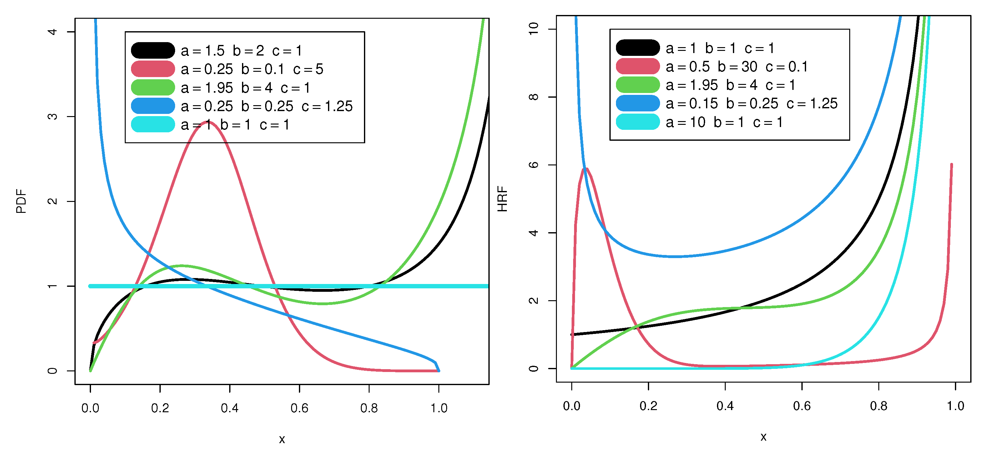
Figure 1 (left) reports some plots of the new PDF. Figure 1 (right) displays some graphs of the new HRF. Figure 1 (left) reveals that the new PDF can be increasing upside-down, unimodal with a right tail, with no peak with a right tail, or uniform. Figure 1 (right) reveals that the new HRF can be increasing monotonically, upside-down U shape, increasing upside-down, U shape (bathtub), or J shape.

The paper is organized as follows. In Section 2, we obtain some properties of the ExKw distribution. In Section 3, we address risk analysis and statistical modeling in the context of insurance, finance, and reliability applications. In Section 4, we present a risk analysis based on a dataset collected from measurements of petroleum rock samples. Different estimation methods and simulations of the new model are discussed in Section 5. Two applications to two real data points empirically show the importance of the ExKw model in Section 6. Many parametric regression models are widely used to explain proportional data. Then, we define the ExKw regression model and provide applications in Section 7. Some conclusions and future works are offered in Section 8.

2. Structural Properties

Let $x\sim$ExKw$(a,b,c)$ be a random variable with PDF (3).

2.1. Asymptotics

The asymptotics of (2)–(4) as $x\to 0^{+}$ are

$$\begin{array}{c}\hfill F\left(x\right)\sim b{x}^a,f\left(x\right)\sim ab{x}^{a-1},h\left(x\right)\sim {\displaystyle \frac{ab{x}^{a-1}}{1-b{x}^a}}.\end{array}$$

The asymptotics of (2)–(4) as $x\to 1^{-}$ are

$$\begin{array}{c}\hfill 1-F\left(x\right)\sim a^c{(1-x)}^c,f\left(x\right)\sim c{a}^c{(1-x)}^{c-1},h\left(x\right)\sim {\displaystyle \frac{c}{1-x}}.\end{array}$$

2.2. Moments

The nth ordinary moment (for any $n>0$) of X is

$$\begin{array}{ccc}& & {\mu }_n^{\prime }=n{\int }_0^1{x}^{n-1}\left[1-F\left(x\right)\right]dx=r{\int }_0^1{\displaystyle \frac{x^{n-1}{(1-x^a)}^c}{1-{(1-x^a)}^b+{(1-x^a)}^c}}dx\hfill \\ & =& n\sum _{i=0}^{\infty }{\int }_0^1{x}^{n-1}{(1-x^a)}^c{\left[{(1-x^a)}^b-{(1-x^a)}^c\right]}^{i}dx\hfill \\ & =& {\displaystyle \frac{n}{a}}\sum _{i=0}^{\infty }\sum _{j=0}^i{(-1)}^j\left({\displaystyle \genfrac{}{}{0pt}{}{i}{j}}\right)B\left({\displaystyle \frac{n}{a}},(j+1)c+(i-j)b+1\right),\hfill \end{array}$$

(5)

where $B(a,b)={\int }_0^1{z}^{a-1}{(1-z)}^{b-1}dz$ is the beta function.

The nth incomplete moment (for any $n>0$) of X, namely $m_n\left(x\right)=E\left(X^n\right|X<x)$, reduces to

$$\begin{array}{ccc}& & m_n\left(x\right)={\displaystyle \frac{a}{F\left(x\right)}}{\int }_0^x{\displaystyle \frac{z^{n+a-1}{(1-z^a)}^{c-1}\left[c+(b-c){(1-z^a)}^b\right]}{{\left[1-{(1-z^a)}^b+{(1-z^a)}^c\right]}^2}}dz\hfill \\ & =& {\displaystyle \frac{a}{F\left(x\right)}}\sum _{i=0}^{\infty }\sum _{j=0}^i{w}_{i,j}{\int }_0^x{z}^{n+a-1}{(1-z^a)}^{(j+1)c+(i-j+1)b-1}\left[c+(b-c){(1-z^a)}^b\right]dz,\hfill \end{array}$$

(6)

where $w_{i,j}=(i+1){(-1)}^j\left({\displaystyle \genfrac{}{}{0pt}{}{i}{j}}\right)$. Finally,

$$\begin{array}{ccc}& & m_n\left(x\right)={\displaystyle \frac{c}{F\left(x\right)}}\sum _{i=0}^{\infty }\sum _{j=0}^i{w}_{i,j}B\left(x^a;{\displaystyle \frac{n}{a}}+1,(j+1)c+(i-j)b\right)\hfill \\ & & +{\displaystyle \frac{b-c}{F\left(x\right)}}\sum _{i=0}^{\infty }\sum _{j=0}^i{w}_{i,j}B\left(x^a;{\displaystyle \frac{n}{a}}+1,(j+1)c+(i-j+1)b\right),\hfill \end{array}$$

(7)

where $B(y;a,b)={\int }_0^y{z}^{a-1}{(1-z)}^{b-1}dz$ is the incomplete beta function.

2.3. Entropy

The cumulative entropy of X, namely $CE\left(X\right)=-{\int }_0^{1}F\left(x\right)log\left[F\left(x\right)\right]dx$, after some simple algebraic manipulation using geometric and generalized binomial expansions, can be written as

$$CE\left(X\right)=S_1+S_2+S_3+S_4,$$

where

$$\begin{array}{ccc}& & S_1=\sum _{i,j=0}^{\infty }\sum _{k=0}^j{\displaystyle \frac{{(-1)}^k\left({\displaystyle \genfrac{}{}{0pt}{}{j}{k}}\right)B\left(\frac{1}{a},(i+j-k+1)b+kc+1\right)}{(i+1)a}},\hfill \\ & & S_2=-\sum _{i,j=0}^{\infty }\sum _{k=0}^j{\displaystyle \frac{{(-1)}^k\left({\displaystyle \genfrac{}{}{0pt}{}{j}{k}}\right)B(\frac{1}{a},(i+j-k+2)b+kc+1)}{(i+1)a}},\hfill \\ & & S_3=\sum _{i,j=0}^{\infty }\sum _{k=0}^{i+j}{\displaystyle \frac{{(-1)}^k\left({\displaystyle \genfrac{}{}{0pt}{}{j}{k}}\right)B(\frac{1}{a},(i+j-k)b+kc+1)}{(i+1)a}},\hfill \\ & & S_4=-\sum _{i,j=0}^{\infty }\sum _{k=0}^{i+j}{\displaystyle \frac{{(-1)}^k\left({\displaystyle \genfrac{}{}{0pt}{}{j}{k}}\right)B(\frac{1}{a},(i+j-k+1)b+kc+1)}{(i+1)a}}.\hfill \end{array}$$

The cumulative residual entropy of X, namely $CRE\left(X\right)=-{\int }_0^1[1-F\left(x\right)]log[1-F\left(x\right)]dx$, reduces to

$$\begin{array}{c}\hfill CRE\left(X\right)=\sum _{i,j=0}^{\infty }\sum _{k=0}^j{\displaystyle \frac{{(-1)}^{j+k}\left({\displaystyle \genfrac{}{}{0pt}{}{-i-2}{j}}\right)\left({\displaystyle \genfrac{}{}{0pt}{}{j}{k}}\right)B(\frac{1}{a},(i+j-k+1)b+(k+1)c+1)}{(i+1)a}}.\end{array}$$

3. Risk Indicators

In recent years, the use of distributions in risk analysis has increased, particularly in finance, insurance, reinsurance, and others. Recently, Hamedani et al. (2023) [7] and Yousof et al. (2024) [8] introduced an extended reciprocal distribution for risk analysis. Alizadeh et al. (2023) [9] and Alizadeh et al. (2024) [10] explored the extended Gompertz model to extreme stress data. Elbatal et al. (2024) [11] proposed a new model for loss and revenue analysis, integrating entropy principles and case studies. For more details, see McNeil et al. (1997) [12], Hogg and Klugman (2009) [13], Jordan and Katz (2018) [14], Martínez-Ruiz (2018) [15], Korkmaz et al. (2018) [16] and Ibrahim et al. (2023) [17].

3.1. The VaR [$q;\widehat{a},\widehat{b},\widehat{c}$] Indicator

The Value-at-Risk (VaR) indicator of X at a confidence level q for the ExKw distribution follows when its CDF equals q. This involves identifying the threshold below which the worst $(1-q)\times 100\%$ of losses are expected, which is a crucial measure to understand and manage extreme risk in financial contexts. The VaR of X is

$$F\left(x_{\mathrm{VaR}\left[q;\widehat{a},\widehat{b}\right]};a,b,c\right)=q,$$

(8)

which is useful for model relevance and sensitivity tests.

3.2. The TVaR $\left[q;\widehat{a},\widehat{b},\widehat{c}\right]$ Indicator

By definition, the Tail Value-at-Risk, or TVR$\left[q;\widehat{a},\widehat{b}\right]$, of X has the form

$$\mathrm{TVaR}=\mathrm{TVaR}\left[q;\widehat{a},\widehat{b},\widehat{c}\right]={\displaystyle \frac{1}{1-\mathrm{VaR}\left[q;\widehat{a},\widehat{b},\widehat{c}\right]}}\mathbf{I}\left(\mathrm{VaR}\left[q;\widehat{a},\widehat{b},\widehat{c}\right];1|q\right),$$

(9)

where

$$\mathbf{I}\left(\mathrm{VaR}\left[q;\widehat{a},\widehat{b},\widehat{c}\right];\infty |q\right)={\int }_{\mathrm{VaR}\left[q;\widehat{a},\widehat{b},\widehat{c}\right]}^{1}xf\left(x;a,b,c\right)dx.$$

(10)

The integral (10) can be found by numerical methods.

3.3. MoP Analysis

The MoP analysis is a robust method for finance and risk assessment to examine the central tendencies and key characteristics of a dataset by analyzing its moments. This technique involves raising each data point to a positive power integer P and calculating the mean of these transformed values, offering insights of various aspects of the data. The choice of P (known as MoP analysis) determines the moments to be analyzed, such as the mean, variance, skewness, or higher moments. This selection affects how different data characteristics, including tail behavior and extreme values, are represented, which is essential for risk evaluation. As discussed by Alizadeh et al. (2024) [10], varying P provides a more thorough analysis, often employing multiple values of P (e.g., $P\in I^{+}=1,2,\dots$) to evaluate the influence of different moments on the dataset. The MOP is defined as

$$\mathrm{MoP}={\left({\displaystyle \frac{1}{n}}\sum _{i=1}^n{x}_i^P\right)}^{{\displaystyle \frac{1}{P}}},$$

where $x_i$ represents the individual data points, n is the total number of observations, and P is the order. For $P=1$, we have the arithmetic mean; for $P=2$, the quadratic mean, also known as the root mean square; and for $P=0$, the geometric mean, but not strictly defined in the MOP framework, only applicable when all $x_i>0$. The MoP becomes more sensitive to extreme values when P increases. For example, the quadratic mean ($P=2$) gives more weight to larger values compared to the arithmetic mean.

The steps for calculating PORT-VaR$\left[q;\widehat{a},\widehat{b}\right]$ include the following:

(1)

Choose the threshold: Determine the threshold T_h based on the data.

(2)

Identify exceedances: Filter the dataset to find all values greater than $T_h$.

(3)

Count exceedances: Calculate the total number of exceedances.

(4)

Estimate the empirical CDF: Calculate the empirical CDF for the exceedances.

(5)

Calculate VaR: Use the empirical distribution of exceedances to find VaR$\left[q;\widehat{a},\widehat{b}\right]$.

3.4. The PORT-VaR$\left[q;\widehat{a},\widehat{b}\right]$ Indicator

PORT-VaR is a sophisticated method utilized in financial risk analysis, which extends the traditional concept of VaR, based on a confidence interval. In essence, VaR provides a statistical measure that indicates the worst expected loss under normal market conditions over a set time frame, allowing financial institutions to gauge their exposure to potential downturns. However, while this indicator is useful for assessing regular market fluctuations, it may not adequately capture the risk associated with extreme losses, which is where PORT-VaR becomes particularly valuable. Using this indicator, we can cope with situations beyond the usual fluctuations captured by standard VaR. This capability enables organizations to implement more robust risk management strategies. Furthermore, PORT-VaR plays a crucial role in ensuring compliance with regulatory requirements, particularly those related to capital reserves. Regulatory bodies often mandate that financial institutions maintain adequate capital against potential extreme loss scenarios to promote stability and protect against systemic risks. For more in-depth information and detailed methodologies related to PORT-VaR, see Alizadeh et al. (2024) [10]. The steps for calculating PORT-VaR include the following:

• Choose the threshold: Determine the threshold from the data or domain knowledge.
• Identify exceedances: Filter the data to find all values greater than the threshold.
• Count exceedances: Calculate the total number of exceedances.
• Estimate the empirical CDF: Calculate the empirical CDF for the exceedances.
• Calculate VaR: Use the empirical distribution of exceedances to find VaR.

4. Risk Analysis

We present a risk analysis based on a dataset collected from measurements of petroleum rock samples. This dataset includes 48 rock samples sourced from a petroleum reservoir, comprising twelve core samples taken from four different cross-sections. Each core sample underwent permeability testing, and the dataset includes measurements for several variables within each cross-section: the total pore area, the total pore perimeter, and the shape of the pores. Furthermore, we analyze the relationship between the shape perimeter and the squared area variable. The importance of risk analysis using methods such as VaR, MOP, PORT-VaR, and TVaR for petroleum rock data is significant for several reasons; see Alizadeh et al. (2024) [10]. and Yousof et al. (2024) [8]. Due to Elbatal et al. (2024) [11], the PORT-VaR quantifies the potential loss in value of an investment portfolio due to adverse market movements. In the context of petroleum rock samples, it can evaluate the financial risk associated with extracting oil from a specific reservoir. By assessing the volatility and expected returns based on the dataset, stakeholders can better understand their potential financial exposure. The MoP can provide insights into average performance of a particular characteristic within the dataset, such as permeability or pore characteristics. By analyzing different moments (e.g., mean, variance), decision makers can gauge the reliability of the samples, which aids in planning extraction strategies and resource allocation. Risk analysis helps to capture the inherent variability in the data. Understanding how different rock samples behave in terms of permeability and other properties can inform predictions about overall reservoir performance and yield. Both MOP and PORT-VaR can facilitate scenario analysis, allowing analysts to simulate various conditions and their impact on reservoir performance. This can help to evaluate “what-if” scenarios related to changes in market prices, extraction technologies, or regulatory environments. Investors can use these risk analyses to make informed decisions about where to allocate capital. By understanding the risk–return profiles of different petroleum reservoirs based on the data, investors can optimize their portfolios and minimize risks.

Friedman and Sotero (2012) [1] underscore the critical role of risk analysis and management within the petroleum industry. Their work highlights the inherent uncertainties associated with oil and gas extraction, emphasizing that effective risk management strategies are essential for optimizing operations and ensuring safety. By integrating statistical methodologies with practical risk management frameworks, their research provides valuable insights that can aid industry professionals in navigating the complex landscape of petroleum production. This study serves as a foundational reference for understanding how statistical analysis can be utilized to mitigate risks and enhance decision-making processes. Chikhi (2016) [2] contributes significantly to the field by exploring the application of the Kw distribution in analyzing petroleum reservoir data. This study illustrates the flexibility and effectiveness of this model in capturing the unique characteristics of geological data, which often exhibit non-standard behaviors. By demonstrating how this distribution can be used to model risks associated with petroleum reservoirs, Chikhi’s research enriches the statistical toolkit available to practitioners. The findings advocate for the adoption of more sophisticated statistical approaches in petroleum engineering, thereby enhancing the accuracy of risk assessments and ultimately improving operational efficiency. Pérez and Del Río (2019) provided a comprehensive review of statistical modeling in petroleum engineering, highlighting the advancements and methodologies that have emerged in recent years. Their analysis not only identifies the various statistical techniques used in the industry but also underscores the importance of integrating these models with real-life applications. By bridging the gap between theoretical developments and practical applications, their research serves as a vital resource for professionals seeking to apply statistical methods in risk assessment. The emphasis on statistical modeling in their work further encourages the incorporation of data-driven decision-making processes, which are essential to address complexities and uncertainties inherent in petroleum exploration and production.

4.1. MoP Analysis for the Petroleum Rock Sample

Table 1. Findings for unit capacity factor data.

$\mathit{P}\uparrow$	$1,2,3,4,5$
TMV	0.2181104
MOO $[P\uparrow ]$	0.0903296, 0.1020908, 0.1070815, 0.1109154, 0.1153489
MSE	0.01632794, 0.01346055, 0.01232742, 0.01149077, 0.01055993
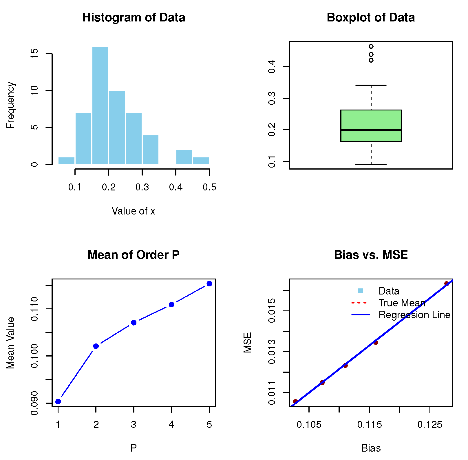
Bias	0.1277808, 0.1160196, 0.1110289, 0.107195, 0.1027615

provides a comprehensive assessment of the MoP under varying values of P (from 1 to 5) for the measurements of petroleum rock samples. This table is crucial for understanding the statistical properties and behavior of the dataset, as it illustrates how different moments capture the underlying characteristics of the rock samples. The TMV value of 0.2181104 serves as a baseline measure of variability in the dataset. This figure reflects the total dispersion of the measurements and provides context for interpreting the subsequent MoP and MSE values. A higher TMV indicates greater variability among samples, which is significant for assessing the performance of the reservoir. The MoP values show a consistent upward trend as P increases. The values range from 0.0903296 for $P=1$ to 0.1153489 for $P=5$. The increase in MoP can indicate a growing emphasis on higher-order characteristics, which are relevant in geological and petroleum studies. The MSE values give a downward trend, ranging from 0.01632794 for $P=$1 to 0.01055993 for $P=5$. This decreasing pattern suggests that the estimates become more accurate as higher moments are considered. A lower MSE indicates improved model fit and reliability of the estimates, which is essential to make sound decisions regarding reservoir management and extraction strategies. The bias values also show a decreasing trend, starting from 0.1277808 for $P=1$ and dropping to 0.1027615 for ($P=5$). This reduction in bias indicates that the models are increasingly aligned with the true underlying parameters of the data. Minimizing bias is critical in statistical modeling, as it enhances the credibility of the estimates.

Furthermore, Table 1 provides valuable insights into the statistical behavior of the petroleum rock data. The consistent trends in the MoP, MSE, and bias values underline the advantages of using higher-order moments for analysis. As P increases, the analysis captures more nuanced aspects of the data, improving both accuracy and reliability. These findings can inform petroleum engineers and geologists in their evaluations of reservoir properties, guiding decisions related to resource extraction and management. The reduced MSE and bias with increasing P shows that employing higher-order moment analysis can provide better informed and more effective strategies in the exploration and production of petroleum resources. Overall, Table 1 highlights the importance of advanced statistical measures in enhancing our understanding of complex geological data. Figure 2 reports the histogram, box plot, MoPs, and biases versus MSE plot for the current data. Figure 3 displays MSEs and biases versus P for these data.

4.2. PORT-VaR$\left[q;\widehat{a},\widehat{b}\right]$ Estimator for Petroleum Rock Data

Table 2. VaR , TVaR, and PORT-VaR$\left[q;\widehat{a},\widehat{b},\widehat{c}\right]$ for petroleum rock data.

CLs ↓	PORT Analysis
	VaR	TVaR	N. of PORT	Min.; 1st Qu.; Median; ExV; 3rd Qu.; Max.
55%	0.201	0.286	26	0.192; 0.210; 0.258; 0.273; 0.307; 0.464
60%	0.208	0.299	29	0.183; 0.201; 0.240; 0.264; 0.291; 0.464
65%	0.229	0.308	31	0.177; 0.200; 0.232; 0.258; 0.286; 0.464
70%	0.239	0.318	33	0.167; 0.198; 0.230; 0.253; 0.281; 0.464
75%	0.263	0.335	36	0.162; 0.188; 0.227; 0.245; 0.277; 0.464
80%	0.276	0.356	38	0.154; 0.183; 0.215; 0.241; 0.276; 0.464
85%	0.291	0.365	40	0.151; 0.179; 0.204; 0.236; 0.276; 0.464
90%	0.327	0.399	43	0.145; 0.170; 0.201; 0.230; 0.269; 0.464
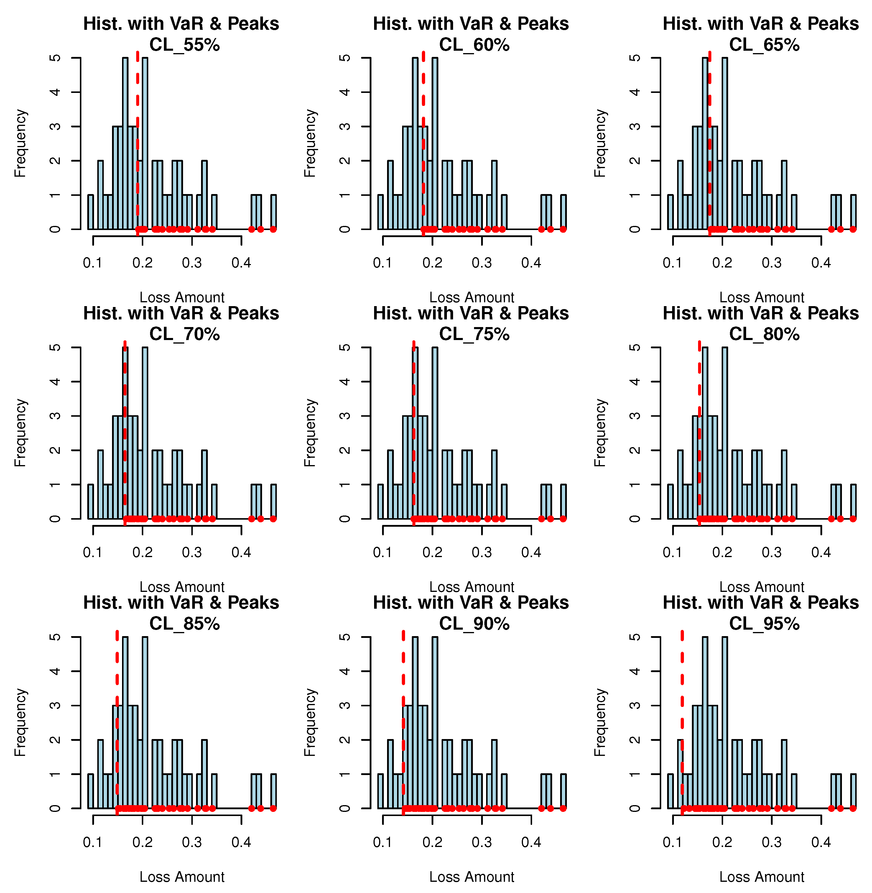
95%	0.393	0.441	45	0.122; 0.164; 0.200; 0.226; 0.263; 0.464

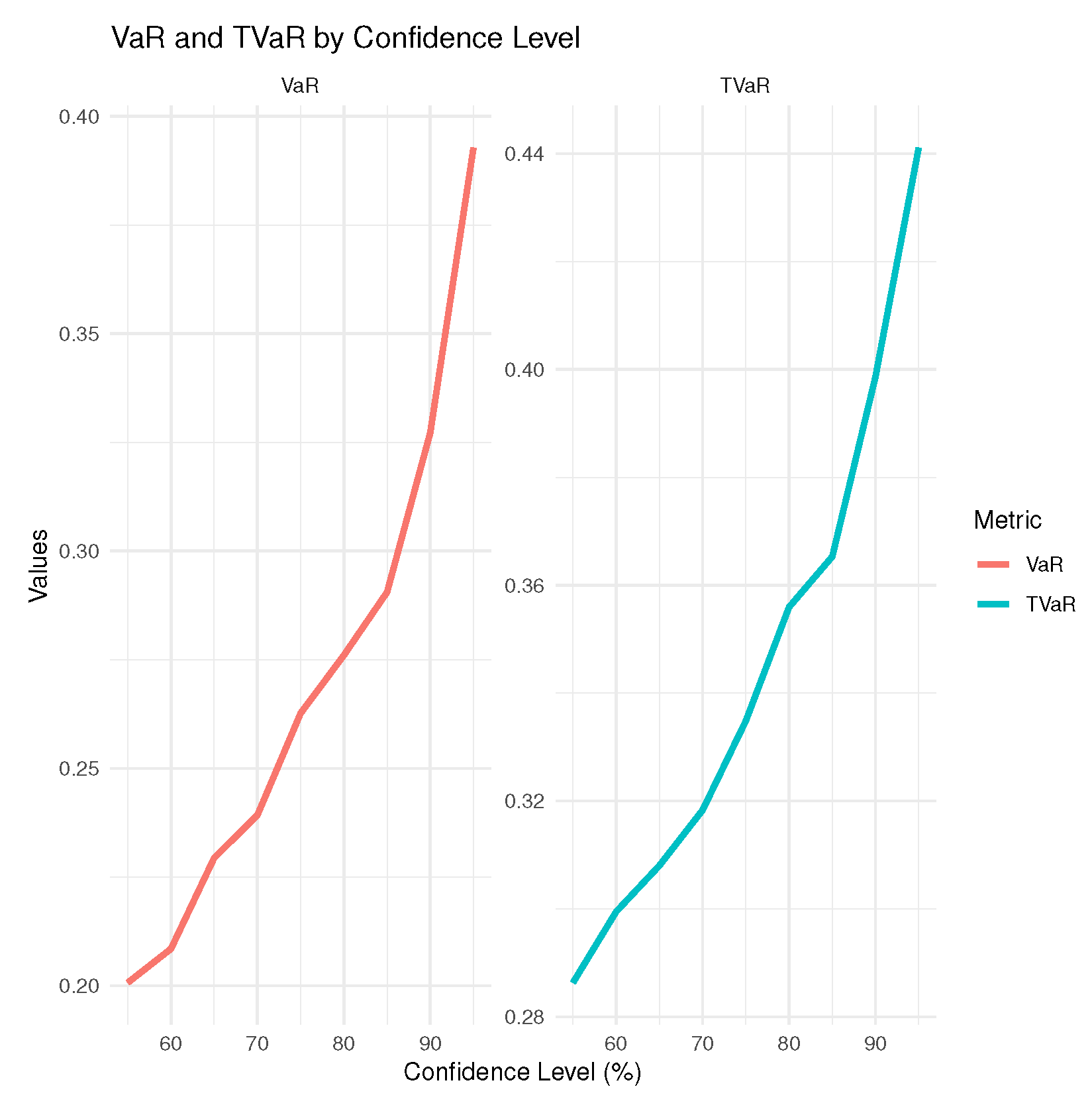
provides risk analysis using VaR, TVaR, and PORT-VaR $\left[q;\widehat{a},\widehat{b}\right]$ for petroleum rock data. It gives results according to some confidence levels (CLs) ranging from 55% to 95%, providing information on the potential risks associated with the dataset. The confidence levels are listed in the first column, indicating the percentage of time in which the losses are expected to be below the specified VaR threshold. As the confidence level increases, the VaR and TVaR values generally increase, reflecting higher risk thresholds. The VaR values increase with higher confidence levels, ranging from 0.2006995 at 55% to 0.3927556 at 95%. The rising trend highlights the increasing potential risk as we consider more extreme scenarios. The TVaR values also show an upward trend, starting at 0.2863168 for 55% and reaching 0.4411047 for 95%. The TVaR metric is particularly important for understanding the potential severity of extreme losses in the tail of the distribution. The number of PORT values increases with higher confidence levels from 26 at 55% to 45 at 95%. This represents the number of observations that fall within the calculated risk thresholds, indicating a growing sample size of extreme cases as confidence increases. It gives some descriptive statistics, including the minimum and maximum, expected value (ExV), and quartiles for the data. These statistics help us to understand the distribution of the data. The minimum values decrease when the confidence level increases, thus indicating that more extreme values are being captured. The median remains relatively stable but shifts upwards with higher confidence levels, reflecting an overall increase in the central tendency of the data. The maximum value remains constant at 0.4641 across all confidence levels, suggesting a capped extreme loss scenario in the dataset.

Also, Table 2 highlights the risks associated with the measurements of petroleum rock samples for some statistical metrics. The consistent increases in VaR and TVaR values with higher confidence levels underscore the importance of considering risk in the management of petroleum resources. Understanding these metrics can help engineers and geologists in anticipating potential losses, allowing them for strategies and operational practices. These statistics offer a comprehensive view of data behavior and help specialists to recognize the variability and potential extreme outcomes associated with petroleum rock samples. This detailed risk assessment is crucial for developing strategies to mitigate risks, optimize resource extraction, and ensure the sustainability of petroleum operations. Table 2 emphasizes the necessity of robust risk management frameworks in the field of petroleum engineering and geology.

Figure 4 provides the PORT-VaR analysis conducted on the petroleum rock data. It is a comprehensive review of the VaR portfolio, highlighting the potential losses that could be encountered under various market conditions. The PORT-VaR specialists can assess the overall risk associated with the dataset, enabling them to decide on resource management and extraction strategies. Figure 5 displays the VaR and TVaR values for the petroleum rock data. The first measure provides an estimate of the maximum expected loss for a certain confidence level. In contrast, the second one offers insight into the expected loss in scenarios where the loss exceeds the VaR threshold. These metrics provide detailed risk assessment, helping stakeholders to understand both typical and extreme risk scenarios associated with the petroleum reservoir. All plots contribute to a deeper understanding of the risks inherent in petroleum extraction and management. By integrating insights from PORT-VaR analysis, peak density evaluations, and VaR/TVaR metrics, specialists can develop more effective strategies to mitigate risks, optimize resource extraction, and enhance decision-making processes in the petroleum industry.

Based on the insights from Table 1 and Table 2, some recommendations can be made for engineering and geology specialists in the petroleum industry:

• Specialists should incorporate higher-order moment analysis, such as Mean of Order P (MoP), into their standard evaluation practices. This approach enhances the understanding of the dataset’s behavior, capturing nuances that lower-order moments may miss.
• Emphasize methodologies that minimize bias and mean squared error (MSE) in parameter estimation. Techniques that improve accuracy will lead to more reliable predictions and decisions on reservoir characteristics.
• Regularly update statistical models as new data become available. This will help ensure that the analyses remain relevant and reflective of current conditions in the reservoir, thereby improving resource management decisions.
• Use the insights gained from MOO analysis to inform operational strategies and planning. Understanding the distribution of reservoir properties can lead to better extraction techniques and resource allocation.
• Develop and implement comprehensive risk management frameworks that incorporate VaR and TVaR analyses. These metrics provide crucial information about potential losses and help in planning for adverse scenarios.
• Pay particular attention to Tail Value-at-Risk (TVaR) in decision-making. Understanding the potential severity of extreme losses is essential for preparing for worst-case scenarios and ensuring that adequate risk mitigation strategies are in place.
• Improve data collection methods to ensure a robust dataset that captures a wide range of scenarios. The number of observations (N. of PORT) is critical for accurate risk assessment, and increasing the sample size can improve the reliability of the results.
• Provide training and resources to engineering and geology teams on advanced statistical tools and risk assessment methodologies. Empowering staff with the knowledge to interpret and apply these analyses will enhance the organization’s overall analytical capabilities.
• Encourage collaboration between geologists, engineers, statisticians, and data scientists to integrate various types of expertise into the analysis process. This multidisciplinary approach can lead to more innovative solutions and comprehensive risk assessments.
• Incorporate sustainability considerations into risk assessments. Understanding the environmental impact of extraction processes, along with potential economic risks, will help develop more sustainable practices in petroleum operations.

By implementing these recommendations, engineering and geology specialists can enhance their analytical capabilities, improve risk management practices, and make more informed decisions in petroleum resource management. Table 1 and Table 2 reveal the importance of robust statistical analysis in understanding and mitigating risks associated with petroleum extraction.

5. Estimation and Simulations

Let $x_1,\dots ,x_n$ be a complete random sample from the ExKw$(a,b,c)$ distribution. The log-likelihood function for the parameter vector $\theta ={(a,b,c)}^{\top }$ of the ExKw distribution is

$$\begin{array}{ccc}\hfill l\left(\theta \right)& =& na+(a-1)\sum _{i=1}^{n}log\left(x_i\right)+(c-1)\sum _{i=1}^{n}log(1-x_i^a)+\sum _{i=1}^{n}log[c+(b-c){(1-x_i^a)}^b]-\hfill \\ & & 2\sum _{i=1}^{n}log[1-{(1-x_i^a)}^b+{(1-x_i^a)}^c].\hfill \end{array}$$

(11)

Equation (11) can be maximized via SAS (Proc NLMixed), R, and the MaxBFGS routine of the matrix programming language Ox.

For the new distribution, we perform simulations to compare six classical estimation methods: Maximum Likelihood Estimation (MLE), Ordinary Least Squares Estimation (LSE), Weighted Least Squares Estimation (WLSE), Cramér–von-Mises Estimation (CVM), Anderson–Darling Estimation (ADE), and Right-Tail Anderson–Darling Estimation (RTADE), with $N=10,000$ Monte Carlo replications each. The MLE maximizes (11) and provides asymptotically unbiased and efficient estimates. The LSE method minimizes the residual sum of squares ${\sum }_{i=1}^n{\left(y_i-\widehat{y_i}\right)}^2$. Under the assumption of normally distributed errors, LSE is both unbiased and efficient. The WLSE method is useful when the variance of the observations is not constant (heteroscedasticity). It minimizes ${\sum }_{i=1}^n{w}_i{\left(y_i-\widehat{y_i}\right)}^2$, where $w_i$ are weights based on the inverse of the variance of the observations. This non-parametric method assesses the goodness-of-fit by evaluating the empirical distribution function. The ADE focuses on the tails of the distribution, thus providing a more sensitive fit in the presence of outliers. Finally, the RTADE method is specifically designed to fit distributions in the right tail, which is crucial for extreme value analysis.

We focus on two primary metrics, bias and root mean squared error (RMSE), to evaluate these estimation methods. By analyzing these metrics across different methods through graphical simulations, we highlight the strengths and weaknesses of each technique in various scenarios, offering valuable guidance to practitioners in selecting suitable estimation methods for their specific requirements.

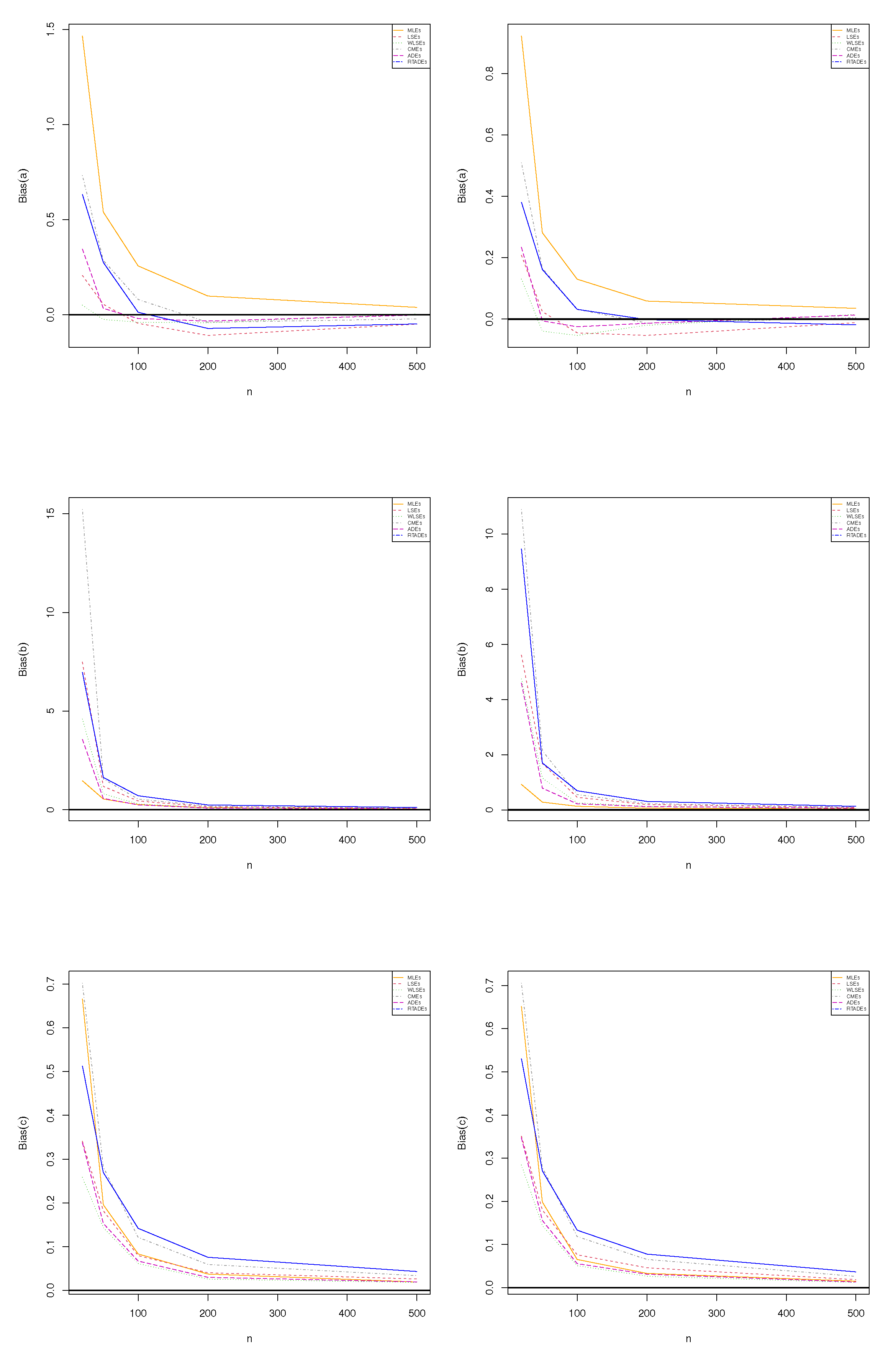
We provide a graphical simulation study by taking into account some assumptions, including two sets of initial values, namely set 1: $(a_0,b_0,c_0)=(2,0.5,1.5)$ and set 2: $(a_0,b_0,c_0)=(1.2,0.5,1.5).$ Figure 6 (the first row) reports the biases for parameter a|$a_0=2$ (left) and a|$a_0=1.2$ (right). Figure 6 (the second row) gives the biases for parameter b|$b_0=0.5$ (left) and b|$b_0=0.5$ (right). Figure 6 (the third row) presents the biases for parameter c|$c_0=1.5$ (left) and c|$c_0=1.5$ (right). 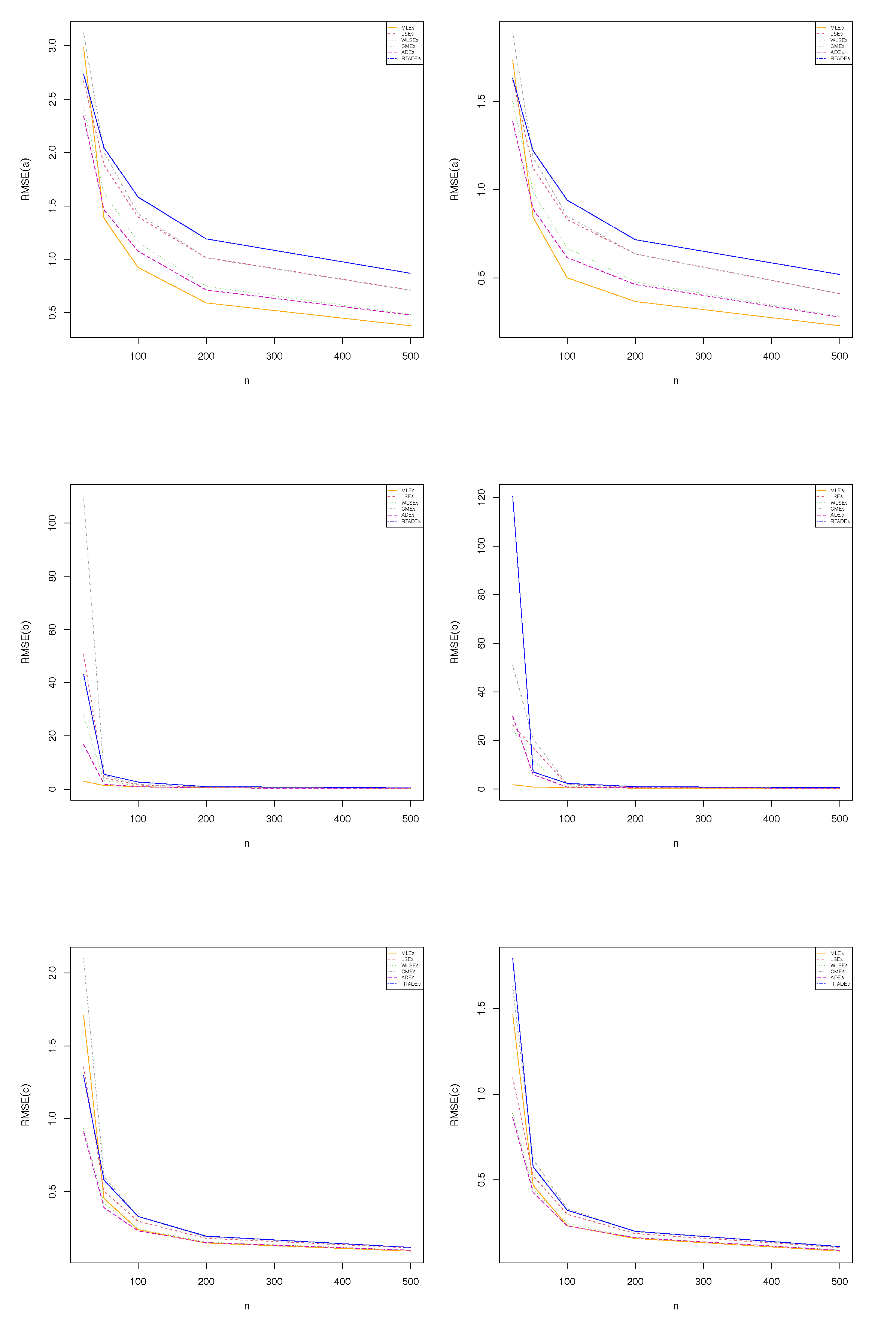Figure 7 (the first row) presents the RMSE for parameter a|$a_0=2$ (left) and a|$a_0=1.2$ (right). Figure 7 (the second row) gives the RMSE for parameter b|$b_0=0.5$ (left) and b|$b_0=0.5$ (right). Figure 7 (the third row) provides the RMSE for parameter c|$c_0=1.5$ (left) and c|$c_0=1.5$ (right). Based on Figure 6 and Figure 7, it is noted that the selected estimation methods perform well for various scenarios. Specifically, the biases for all methods tend to approach zero when the sample size increases, thus indicating that the estimates become more accurate and closer to the true parameters. This reduction in bias signifies the consistency and reliability of the methods under consideration. Furthermore, the RMSE also decreases as the sample size grows, reinforcing that larger samples lead to more precise estimates. A reduced RMSE suggests that both the variability and the error of the estimators are minimized, enhancing the overall performance of the methods. This trend highlights the effectiveness of these estimation techniques in drawing reliable conclusions from increasingly larger datasets, making them suitable choices for practitioners seeking robust statistical analysis.

Based on widely accepted guidelines in statistical literature (e.g., Agresti, 2002 [18]), we define standardized thresholds: for bias, $\left|Bias\right|$$<0.05$ is considered negligible, $0.05\le \left|Bias\right|<0.10$ small, $0.10\le \left|Bias\right|<0.20$ moderate, and $\left|Bias\right|\ge 0.20$ large; for RMSE, values less than $0.10$ indicate excellent precision, 0.10–0.20 good, 0.20–0.30 moderate, and above $0.30$ poor. These benchmarks were applied to evaluate the performance of six estimation methods for some sample sizes and parameter configurations. Our findings revealed that bias generally approached zero with increasing sample size, indicating asymptotic unbiasedness, while RMSE decreased, reflecting improved precision, particularly for MLE.

6. Real Data Modeling

The ExKw distribution was applied to two real datasets. The codes are available at https://github.com/gabrielamrodrigues/ExKw (accessed on 27 June 2025). The first one refers to the total milk production from the first lactation of 107 SINDI breed cows. They are owned by the Carnaúba farm, which is part of Agropecuária Manoel Dantas Ltda (AMDA) (Taperoá, a city in the state of Paraíba, Brazil). The researchers aim to gain valuable insights into the milk production characteristics of the SINDI breed. The analysis focuses on understanding the variability in milk yield among cows during their initial lactation period, which can provide important information to improve dairy management practices. This research not only contributes to the optimization of production at the Carnaúba farm but also enhances knowledge about the SINDI breed’s performance in dairy production, potentially benefiting other farmers and stakeholders in the region.

The second one aims to estimate the unit capacity factor, a crucial metric in various engineering and resource management applications. This estimation was previously conducted by Caramanis et al. (1984) [19]. both of whom contributed significantly to the understanding of capacity factors in their respective studies. More recently, Genc (2013) [20] and Arslan (2023) [21] revisited these data, providing further insights on the unit capacity factor, highlighting its relevance in contemporary research. In addition to its historical significance, this dataset serves a dual purpose. It is also adopted to prove the applicability of the new distribution as an alternative to the beta and Kw models. By fitting the ExKw model to these data, researchers can evaluate its effectiveness in capturing the underlying distribution of the unit capacity factor. This exploration not only validates this model but also positions it as a potentially more flexible and robust alternative for modeling data that are typically addressed by beta and Kw distributions. The findings of this analysis could pave the way for broader applications of the ExKw model in various fields, enhancing the precision and reliability of capacity factor estimations.

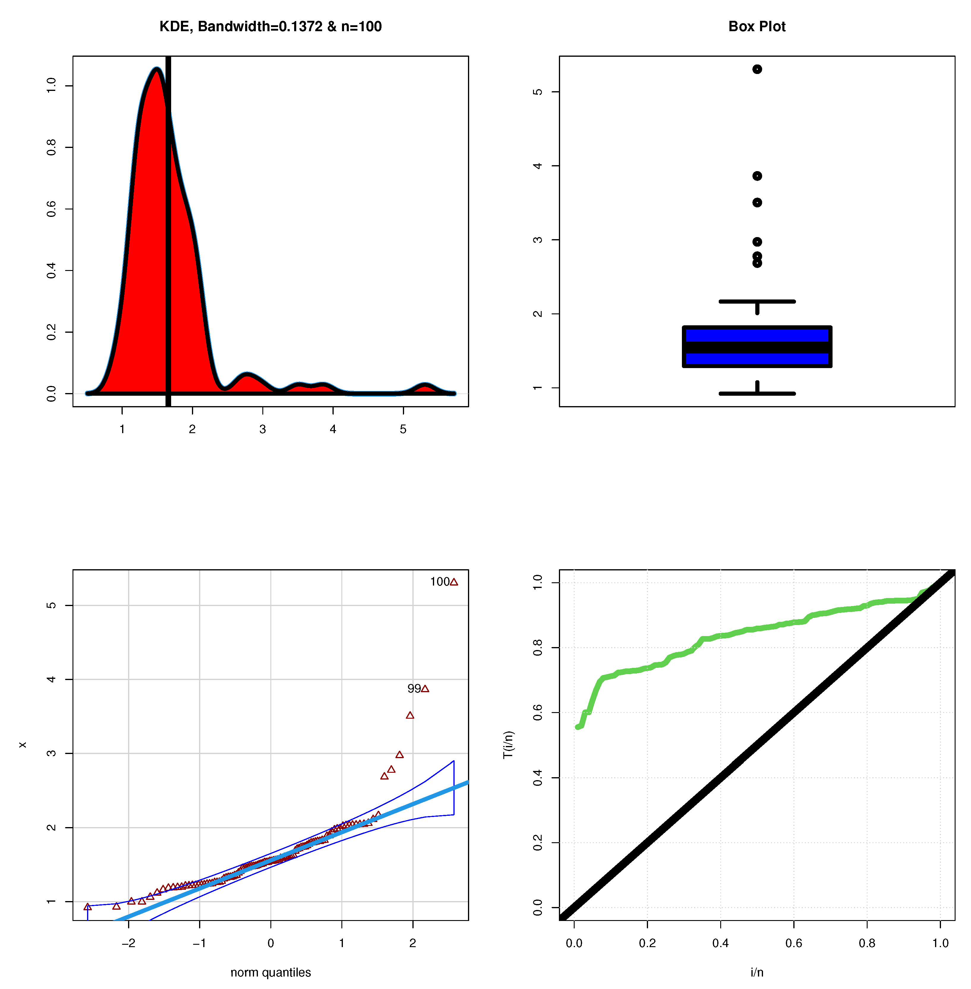
Figure 8 reports some plots to describe milk production. Figure 8 (top left) gives the Kernel plot, and Figure 8 (top right) provides the box plot. Figure 8 (bottom left) gives the QQ plot, and Figure 8 (bottom right) gives the total time in test (TTT) plot. Figure 9 presents some plots to describe the unit capacity factor. Figure 9 (top left) gives the Kernel plot for the unit capacity factor, and Figure 9 (top right) provides the box plot for this unit. Figure 9 (bottom left) gives the QQ plot for the unit, and Figure 9 (bottom right) reports the TTT plot.

Based on Figure 8, the analysis reveals that milk production is right-skewed, indicating that while most cows have lower milk yields, there are a few that produce significantly higher amounts. This right skewness often suggests the presence of a few outliers or extreme values, which can influence the overall distribution. The histogram or density plot likely shows that the majority of the data points cluster towards the lower end, while the tail extends to the right, representing those exceptional cases of high production. Additionally, the HRF associated with these data is monotonically increasing. This means that as milk production increases, the likelihood of achieving higher yields continues to rise, reflecting a positive relationship between the amount produced and the probability of observing greater production levels. In contrast, Figure 9 indicates that the unit capacity factor exhibits a bimodal distribution. This suggests that there are two distinct groups or peaks within the dataset, each representing a different range of capacity factors. Unlike the milk production data, this dataset does not show any extreme values, implying that the observed values are relatively consistent and fall within expected limits. The HRF for the unit capacity factor is also monotonically increasing, indicating that as the capacity factor increases, the probability of observing even higher values continues to grow. This characteristic is essential for understanding how capacity factors behave across different contexts and can provide valuable insights into system performance and efficiency.

Table 3. Descriptive statistics for real datasets.

Data	Mean	Variance	Skewness	Kurtosis
dataset 1	$0.468$	$0.036$	$-0.330$	$-0.363$
dataset 2	$0.303$	$0.101$	$0.663$	$-1.283$

lists the descriptive statistics for both datasets. Milk production data appear to have a more compact distribution with a slight left skew, while data of the unit capacity factor have a wider distribution with a positive skew. The shapes of the distributions can significantly impact how data are analyzed and interpreted. Given the different characteristics, choosing appropriate statistical models will be crucial. The milk production data may be more amenable to models assuming normality, whereas dataset 2 may require consideration of its skewness and greater variability in the modeling process. The characteristics of these datasets could inform different applications. For instance, milk production data may be suitable for scenarios where consistent performance is valued, while unit capacity factor data might be more relevant in situations where outlier detection and variability are important.

Table 4. Findings for milk production.

Model	Estimated Parameters (se)			${\mathit{W}}^{*}$	${\mathit{A}}^{*}$	$\mathit{AIC}$	$\mathit{BIC}$	p-Value
ExKw$(a,b,c)$	$1.019$	$0.261$	$2.880$	$\mathbf{0}.\mathbf{029}$	$\mathbf{0}.\mathbf{220}$	$-\mathbf{52}.\mathbf{50}$	$-\mathbf{44}.\mathbf{48}$	$\mathbf{0}.\mathbf{993}$
	$\left(0.062\right)$	$\left(0.416\right)$	$\left(0.421\right)$
Beta$(a,b)$	$2.412$	$2.829$		$0.208$	$1.362$	$-43.55$	$-38.20$	$0.338$
	$\left(0.314\right)$	$\left(0.374\right)$
Kw$(a,b)$	$2.194$	$3.436$		$0.156$	$1.009$	$-46.78$	$-41.44$	$0.562$
	$\left(0.222\right)$	$\left(0.582\right)$

The model with the best fit measures is indicated in bold.

reports three statistical models (ExKw, Beta, and Kw) along with their estimated parameters, standard errors (SEs), goodness-of-fit statistics, and p-values. The Akaike Information Criterion (AIC) and Bayesian Information Criterion (BIC) are adopted. Each model offers insights of the current data, and the comparison among them can help identify the most appropriate fit. For the ExKw model, AIC = $-52.50$, BIC = $-44.48$, and p-value = 0.993. The ExKw model shows strong performance with the highest p-value (0.993), thus indicating that this model fits the data well without significant evidence against it. The AIC and BIC values are the lowest among the three models, suggesting that this model provides the best balance between goodness of fit and complexity. The SEs of the estimated parameters are relatively low, indicating precise estimates. This model may capture the nuances in the data effectively. However, the beta model shows a moderate fit to the data, with a p-value of 0.338, indicating some evidence against the null hypothesis of fit but still acceptable. The AIC and BIC values are higher for the ExKw model, suggesting that it is less parsimonious. The larger SEs for the estimated parameters indicate less precision compared to the ExKw model, which may affect the reliability of the estimates.

The Kw model has a p-value of 0.562, suggesting a moderate fit, though it is less favorable than the ExKw model. The AIC and BIC values indicate that it offers a better fit than the beta model but not as good as the ExKw model. The SEs for the estimates show reasonable precision but are larger for b, indicating that the estimate for this parameter is less stable. The figures in Table 2 show that the new model is the best one for the data. It effectively balances fit and complexity, providing precise parameter estimates. In contrast, while the beta and Kw models provide reasonable alternatives, they do not perform as well as the ExKw model based on the goodness-of-fit statistics. This analysis suggests that researchers may prefer the ExKw model for its robustness and reliability in modeling the given dataset. 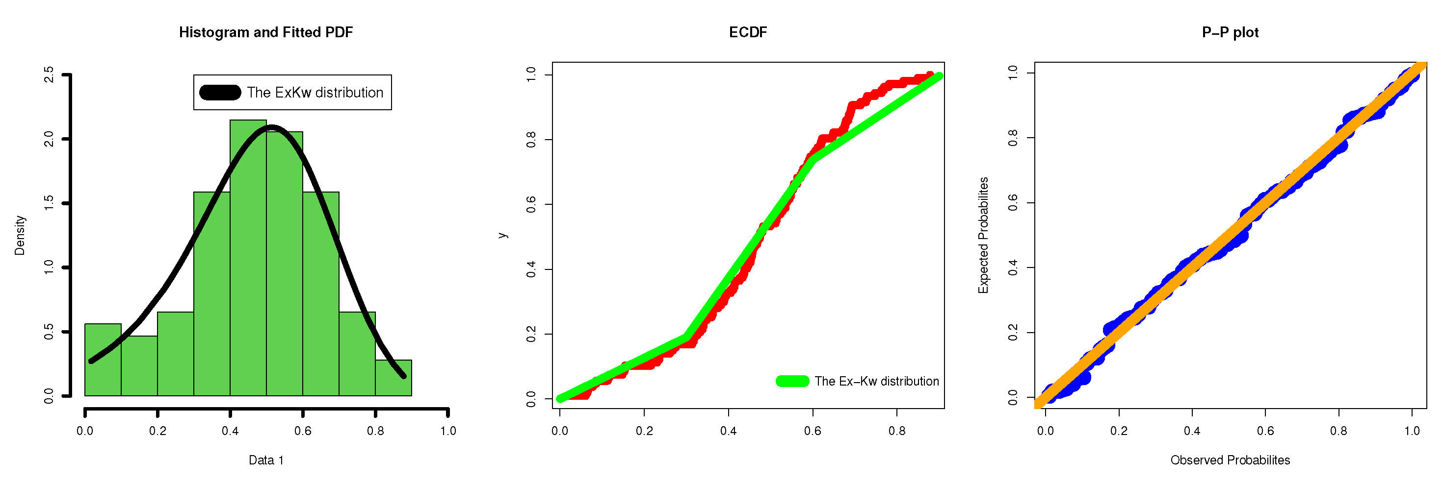On the other hand, Figure 10 displays the estimated PDF and its corresponding estimated CDF (ECDF) for milk production. Figure 11 shows the estimated PDF and its estimated CDF (ECDF) for the unit capacity factor. In general, the graphical results show the importance of the new distribution and demonstrate its flexibility and applicability and that it is a suitable alternative to the beta and Kw distributions.

Table 5. Findings for the unit capacity factor data.

Model	Estimated Parameters (SEs)			${\mathit{W}}^{*}$	${\mathit{A}}^{*}$	$\mathit{AIC}$	$\mathit{BIC}$	p-Value
ExKw$(a,b,c)$	$1.607$	$52.836$	$1.850$	$\mathbf{0}.\mathbf{014}$	$\mathbf{0}.\mathbf{131}$	$-\mathbf{16}.\mathbf{57}$	$-\mathbf{13}.\mathbf{30}$	$\mathbf{0}.\mathbf{999}$
	$\left(0.375\right)$	$\left(58.401\right)$	$\left(0.576\right)$
Beta$(a,b)$	$0.553$	$1.219$		$0.117$	$0.712$	$-9.56$	$-7.38$	$0.341$
	$\left(0.142\right)$	$\left(0.375\right)$
Kw$(a,b)$	$0.571$	$1.230$		$0.115$	$0.703$	$-9.68$	$-7.50$	$0.365$
	$\left(0.147\right)$	$\left(0.348\right)$

The model with the best fit measures is indicated in bold.

presents the ExKw, Beta, and Kw models along with their estimated parameters, SEs, goodness-of-fit statistics, and p-values for the unit capacity factor data. So, the ExKw model has an exceptionally high p-value of 0.999, suggesting an excellent fit to these data with no significant evidence against the model. Its AIC and BIC values are the lowest among the three models, indicating that this model achieves the best trade-off between goodness of fit and complexity. The SEs of the estimates, particularly for b, are relatively large, which may indicate some instability in this estimate, but the model remains robust. The beta model has a p-value of 0.341, indicating some evidence against the null hypothesis of fit, but it is still within an acceptable range. The AIC and BIC values are higher than those of the ExKw model, suggesting that this model is less parsimonious. The SEs of the estimates are relatively low, thus indicating precise estimates, although the lower mean values suggest a shift in the distribution’s center compared to the ExKw model. The Kw model yields a p-value of 0.365, suggesting a moderate fit that is slightly less favorable than the ExKw model but better than the Beta model. The AIC and BIC values are very close to those of the beta model, indicating that it offers similar fit characteristics. The SEs are reasonable, but the parameters indicate that the model captures the lower range of the data well, potentially missing some higher values.

The ExKw distribution clearly emerges as the best model for these data, supported by its lowest AIC and BIC values along with a p-value indicating a strong fit (see Table 5). The beta and Kw models do not match the performance of the ExKw model based on the goodness-of-fit statistics. The model robustness, despite some variability in parameter estimates, makes it a reliable choice for accurately modeling the dataset at hand. Researchers may benefit from its flexibility and fit quality in their analyses.

7. The ExKw Regression Model

We construct the ExKw regression model as a very competitive alternative to the Kw and beta regressions. Let $V={(v_1,\dots ,v_n)}^{\top }$ be a matrix of known explanatory variables, where $v_i^{\top }=(v_{i1},\dots ,v_{ip})$. The ExKw regression model is defined by the density (3) of X and the systematic component

$$\begin{array}{c}\hfill a_i=exp\left(v_i^{\top }{\beta }_1\right),i=1,\dots ,n,\end{array}$$

(12)

and ${\beta }_1={({\beta }_{11},\dots ,{\beta }_{1p})}^{\top }$ is the unknown parameter vector. Note that sometimes problems of non-constant variance in the data may exist (problem of variance heterogeneity), so in this case it is necessary to add another systematic component, so there are two systematic components. Usually, this modeling can be applied to the heterogeneity of the data.

The total log-likelihood function for $\theta ={({\beta }_1^{\top },b,c)}^{\top }$ from a set of independent observations $(x_1,v_1),\dots ,(x_n,v_n)$ is

$$\begin{array}{ccc}\hfill l\left(\theta \right)& =& \sum _{i=1}^n\left(v_i^{\top }{\beta }_1\right)+\sum _{i=1}^n(a_i-1)log\left(x_i\right)+(c-1)\sum _{i=1}^{n}log(1-x_i^{a_i})+\hfill \\ & & \sum _{i=1}^{n}log[c+(b-c){(1-x_i^{a_i})}^b]-2\sum _{i=1}^{n}log[1-{(1-x_i^{a_i})}^b+{(1-x_i^{a_i})}^c].\hfill \end{array}$$

We employ the gamlss package of the R software to maximize $l\left(\theta \right)$, and we obtain the maximum likelihood estimate (MLE) $\widehat{\theta }$ of $\theta$. The fitted normal regression (with $a=b=1$) gives initial values for $\beta$. The classical asymptotic likelihood theory can be used to find confidence intervals for the parameters and goodness-of-fit tests for comparing the ExKw regression model with its special cases.

The quantile residuals (qrs) (Dunn and Smyth, 1996) [22] are adopted to verify the model assumptions. For the ExKw regression model, we obtain

$${\widehat{r}}_{q_i}={\mathsf{\Phi }}^{-1}\left\{{\displaystyle \frac{1-{(1-x_i^{{\widehat{a}}_i})}^{\widehat{b}}}{1-{(1-x_i^{{\widehat{a}}_i})}^{\widehat{b}}+{(1-x^{{\widehat{a}}_i})}^{\widehat{c}}}}\right\},$$

(13)

where ${\mathsf{\Phi }}^{-1}(·)$ is the inverse cumulative standard normal distribution and $a_i=exp\left(v_i^{\top }{\widehat{\beta }}_1\right)$.

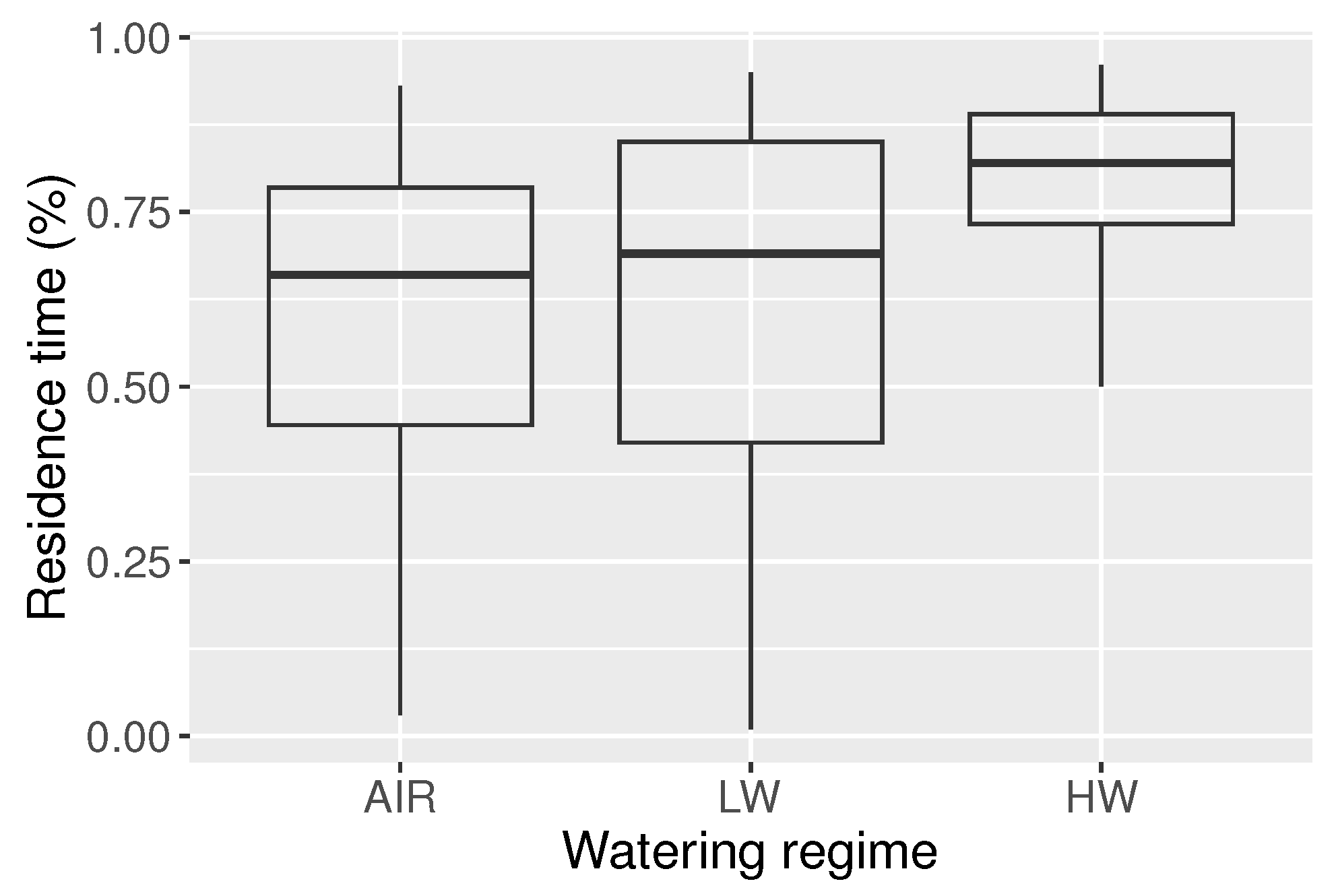
Application: Residence Times

The changes in the attractiveness of a plant–soil system for female herbivorous mosquitoes exposed to some combinations of treatments are reported at the link https://doi.org/10.1016/j.dib.2021.107297. The behavior of females ($n=162$) is described as the residence times (choice versus no-choice) of unidirectional olfactometers, and the variables under study are

• $x_i$: residence time (% of time spent in the choice area/100);
• Watering regime: AIR (clean air), HW (high-watered), and LW (low-watered) defined by the dummy variables $v_{i1}$ and $v_{i2}$ ($i=1,\dots ,162$).

Table 6. Descriptive statistics for residence times.

Treatment	Mean	Median	SD	Min.	Max	Skewness	VC	Kurtosis
AIR	0.60	0.66	0.24	0.03	0.93	−0.71	39.85	2.62
LW	0.60	0.69	0.28	0.01	0.95	−0.74	46.37	2.34
HW	0.76	0.82	0.21	0.08	0.96	−1.93	27.62	6.47

gives descriptive statistics for each watering regime, where there is negative skewness and positive kurtosis for the three treatments. Figure 12 reveals that the HW regime obtained the longest residence times, as well as some outliers.

We consider the following systematic components for the regression models:

$$Systematic=\left\{\begin{array}{c}{\mathcal{M}}_0:log\left({\mu }_i\right)={\beta }_{10};\hfill \\ {\mathcal{M}}_1:log\left({\mu }_i\right)={\beta }_{10}+{\beta }_{11}{v}_{i1}+{\beta }_{12}{v}_{i2}.\hfill \end{array}\right.$$

Table 7. AIC, BIC, and GD of Kw, Beta, and ExKw regression models.

		Kw	Beta	ExKw
${\mathcal{M}}_0$	AIC	−33.12	−33.16	−66.15
	BIC	−26.95	−26.98	−56.88
	GD	−37.12	−37.16	−72.15
${\mathcal{M}}_1$	AIC	−38.55	−47.37	−82.05
	BIC	−26.20	−35.01	−66.61
	GD	−46.55	−55.37	−92.05

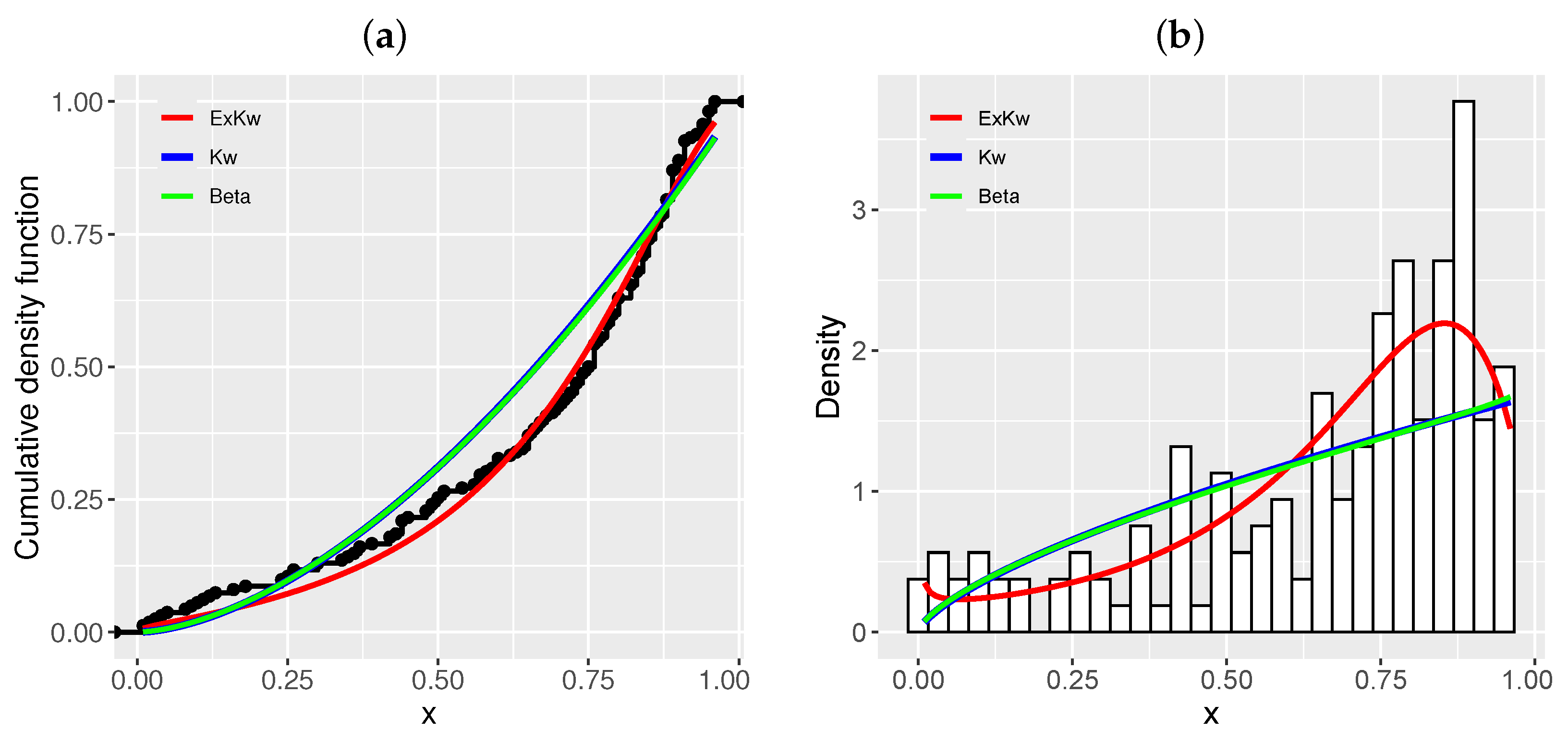
provides the AIC, BIC, and Global Deviance (GD) for six fitted models. The numbers show that the ${\mathcal{M}}_1$-ExKw model is the best one among them. The likelihood ratio (LR) statistic to compare the ${\mathcal{M}}_1$-ExKw and ${\mathcal{M}}_1$-Kw models is 45.5, and the p-value $<0.001$, which supports this conclusion. The plots of the empirical and estimated cumulative distributions in Figure 13a and the histogram and plots of the estimated densities in Figure 13b prove this fact.

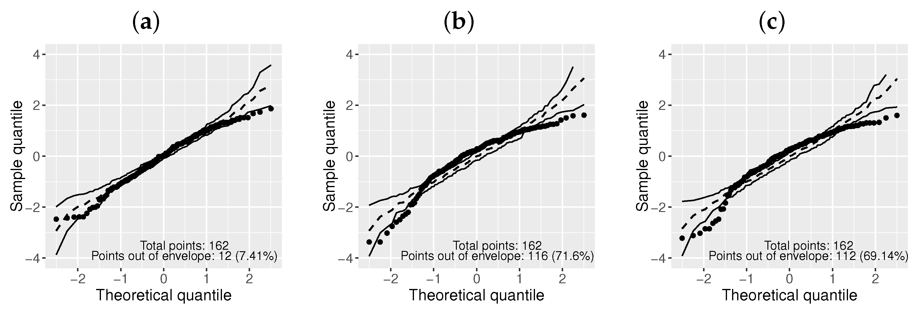
The normal probability plots with simulated envelopes for the ${\mathcal{M}}_1$ models are reported in Figure 14. Clearly, the ${\mathcal{M}}_1$-ExKw model is superior to the others.

The estimates, their SEs, and p-values for the ${\mathcal{M}}_1$-ExKw regression model are listed in

Table 8. Findings from the ${\mathcal{M}}_1$-ExKw regression model.

	MLEs	SEs	p-Values
${\beta }_{10}$	−1.13	0.15	<0.01
${\beta }_{11}$	0.08	0.19	0.66
${\beta }_{12}$	0.78	0.20	<0.01
$log\left(b\right)$	−3.57	0.14
$log\left(c\right)$	0.34	0.05

. So, the high-irrigation regime (parameter ${\beta }_{11}$) is significant relative to clean air, which indicates an increase in residence time with high irrigation compared to clean air. However, the low-irrigation regime is not significant.

8. Conclusions

We introduced a novel unit distribution and provided an in-depth exploration of its properties and advantages. We proved how this distribution can be effectively applied in real-life scenarios, particularly within the field of geology. One of the key applications we explored was the development of a set of risk indicators. These indicators are particularly valuable in estimating risks in geological contexts. We applied the new unit distribution in two geological datasets. The results were compared with the beta and Kumaraswamy distributions. We also explored six estimation techniques for the parameters of the new distribution. Additionally, we constructed a regression model under the novel unit distribution, which was applied in statistical prediction tasks, specifically focusing on residence time data. We were able to make more accurate predictions and gain deeper insights in the dynamics of the processes under study. Our work demonstrates the versatility and utility of the new unit distribution in both theoretical and practical applications, offering promising avenues for future papers and development in this field. In future research, the following topics can be addressed: proposing a regression model for limited ExKw data inflated with zeros and ones; developing a library for the ExKw regression model; constructing an ExKw regression model for correlated data with random effects; and studying and defining residuals for the ExKw regression model, among others.