Continuity Correction and Standard Error Calculation for Testing in Proportional Hazards Models

Abstract

Standard asymptotic inference for proportional hazards models is conventionally performed by calculating a standard error for the estimate and comparing the estimate divided by the standard error to a standard normal distribution. In this paper, we compare various standard error estimates, including based on the inverse observed information, the inverse expected inverse information, and the jackknife. Furthermore, correction for continuity is compared to omitting this correction. We find that correction for continuity represents an important improvement in the quality of approximation, and furthermore note that the usual naive standard error yields a distribution closer to normality, as measured by skewness and kurtosis, than any of the other standard errors investigated.

1. Introduction

Statisticians commonly estimate the parameters in a model through the likelihood. In fully parametric models, the unknown parameter vector is estimated as the log-likelihood maximizer. Denote the log likelihood by ℓ, and the unknown parameter vector by $\mathit{\beta }$; then, the maximum likelihood estimator $\widehat{\mathit{\beta }}$ solves the equation

$${\mathit{\ell }}^{\prime }\left(\widehat{\mathit{\beta }}\right)=0$$

(1)

[1] (Chapter 9).

One often tests hypotheses involving individual parameters by subtracting the null expectation from a parameter estimate, dividing this difference by the square root of an estimate of the variance of the parameter estimate, and comparing this quotient to a standard normal distribution; this test is called a Wald test.

One might calculate a standard error using the inverse of the Fisher information, where the Fisher information is the expected value of the second derivative of the log-likelihood and is written as

$$I=E(-{\mathit{\ell }}^{\prime \prime }\left(\mathit{\beta }\right))$$

(2)

[1] (Chapter 9).

In order to avoid calculating the expectation in (2), one often approximates the expected second derivative of the log-likelihood at the true value by the observed value of the second derivative of the observed log-likelihood evaluated at the observed maximizer [2] (Section 10.3).

Other techniques for calculating standard errors is using a process called jackknife resampling, in which the estimator is adjusted by averaging across each systematic omission of an observation in a one by one fashion [3], and using a resampling technique called the bootstrap [4].

We can use the likelihood to test the effects of covariates on times until an event is complicated by the involvement of the baseline distribution of times in the likelihood. Practitioners often remove this dependency by using the Cox proportional hazards model [5]. In this case, a version of the likelihood reflecting some, but not all, of the variability in the model is used for inference. This likelihood counterpart is called the partial likelihood, and we denote it by ℓ. The Wald test for the null hypothesis that a parameter ${\beta }_j$ takes a null value ${\beta }_j^0$ vs. the alternative hypothesis that ${\beta }_j>{\beta }_j^0$ is performed by taking the root of (1), ${\widehat{\beta }}_j$, calculating its standard error $\mathrm{s}.\mathrm{e}.\left(\widehat{{\beta }_j}\right),$ and comparing

$$({\widehat{\beta }}_j-{\beta }_j^0)/\mathrm{s}.\mathrm{e}.\left(\widehat{{\beta }_j}\right)$$

(3)

to a standard normal distribution. Our simulation, below, shows that the partial likelihood typically underestimates the p-value for the Wald test [6].

When possible values of the score vector ${\ell }^{\prime }\left(\mathit{\beta }\right)$ are discrete, and when the distribution of ${\ell }^{\prime }\left(\mathit{\beta }\right)$ is approximated using a continuous approximation, then values of ${\ell }^{\prime }\left(\mathit{\beta }\right)$ are corrected by moving them half the distance to an adjacent support point of this distribution. This adjustment is called a continuity correction.

In this paper, we explore the qualities of various standard error calculations, as well as the impact of continuity correction on the accuracy of p-value approximations. Since standard errors are used to create a test statistic with a null distribution that is only approximately standard normal, we use the standard normality of the test statistic as our criteria of quality. In practice, a Monte Carlo simulation computes the desired standard errors, which are then compared to the shared exact standard deviation. While extensions of the Cox model to time-dependent factors do exist [7], they are beyond the scope of this paper.

2. Materials and Methods

Symbols describing models for survival data involve are defined in

Table 1. Variables.

Variable Name	Symbol
(Explanatory) Covariates	$\mathbf{x}$
Sample Size	N
profile Number of Covariates	m
Censoring Rate	$\kappa$
Scale Parameter	$\lambda$
Fixed Event Parameter	$\mathit{\beta }$
Event Time	U
Censoring Status	$\delta$
Theoretical Quantile	$\tau$

. Assume that the distribution of latent event time $U_j$ for subject j depends on covariates $x_j^i$. Let $S_j\left(u\right)$ represent the survival function $S_j\left(u\right)=P[U_j\ge u]$, and define the hazard function $h_j\left(u\right)=-{\displaystyle \frac{d}{du}}log\left(S_j\left(u\right)\right)$. Furthermore, censoring times $C_j$ are determined for each subject. Investigators observe the minimum of the censoring and event times, $T_j=min(U_j,C_j)$, and an indicator ${\delta }_j=\left\{\begin{array}{cc}1\hfill & \mathrm{if}{U}_j\le C_j\hfill \\ 0\hfill & \mathrm{if}{U}_j>C_j\hfill \end{array}\right.$.

Cox proportional hazards regression models the hazard function for subject j with covariates $x_j^i$ as

$$h_j(t,{\mathbf{x}}_j)=h_0\left(t\right)exp\left(\sum _{i=1}^p{\beta }_i{x}_j^i\right),$$

(4)

where $h_0\left(t\right)$ corresponds to the baseline hazard function (i.e., when all covariates are zero), $x_j^i$ is covariate i for subject j, and ${\beta }_i$ is component i of the fixed event parameter $\mathit{\beta }$, as in Table 1.

Practitioners generally desire inference on $\mathit{\beta }$, often without inference on $h_0\left(t\right)$. Generally, the partial likelihood is

$$\ell \left(\mathit{\beta }\right)=\sum _{j\in \mathcal{C}}\left[\sum _i{\beta }_i{x}_j^i-log\left(\sum _{m\in \mathcal{R}\left(j\right)}exp\left(\sum _i{\beta }_i{x}_m^i\right)\right)\right],$$

where $\mathcal{C}=\left\{j\right|{\delta }_j=1\}$ is the set of subjects who have the event and $\mathcal{R}\left(j\right)=\left\{m\right|U_m\ge U_j\}$ is the set of subjects at risk of having the event when subject j has the event. This simulation produces a data set allowing the estimation of coverage probabilities. Appendix A (Simulation Details) in the appendix provides implementation details that supplement the following overview. The computer code may be found at https://github.com/dbaumg/Gaussian-Approx-Proportional-Hazards (accessed on 20 April 2025).

2.1. Assessment of Frequency Properties of Estimates via Simulation

As mentioned, simulations presented here are performed on two levels. We first describe the outer simulation, which is parameterized by inputs N, m, $\lambda$, $\beta$, and $\kappa$. These govern the process that generates data sets indexed by i (running from 1 to N) that maintain time, status, and covariate values. A vector $\mathit{\beta }$ is constructed with m entries, where each entry is set to $\beta$.

The N covariate vectors x were generated as independent m-variate standard normal variables. Weibull latent event times were obtained using a sample of size N from the uniform distribution; for subject j, call this random quantity $V_j$. The latent times themselves were calculated as

$$U_j={\displaystyle \frac{-log\left(V_j\right)}{\lambda ·exp\left({\sum }_{i=1}^p{\beta }_i{x}_j^i\right)}}.$$

The parameter vector $\mathit{\beta }$ and the vector of covariates $\mathbf{x}$ have the same number of components, and their contributions were combined with a dot product. The censoring mechanism used a random sample of size N from the exponential distribution (using $\kappa$). These were each increased by $log\left(2\right)/\lambda$, and the obtained value is the censoring time C. We compute the time for subject j as $T_j=min(U_j,C_j)$, we can define ${\delta }_j$ so that it indicates censoring:

$${\delta }_j=\left\{\begin{array}{cc}0\hfill & U\le C_j\hfill \\ 1\hfill & U_j>C_j\hfill \end{array}\right..$$

2.2. Evaluating and Comparing Standard Errors

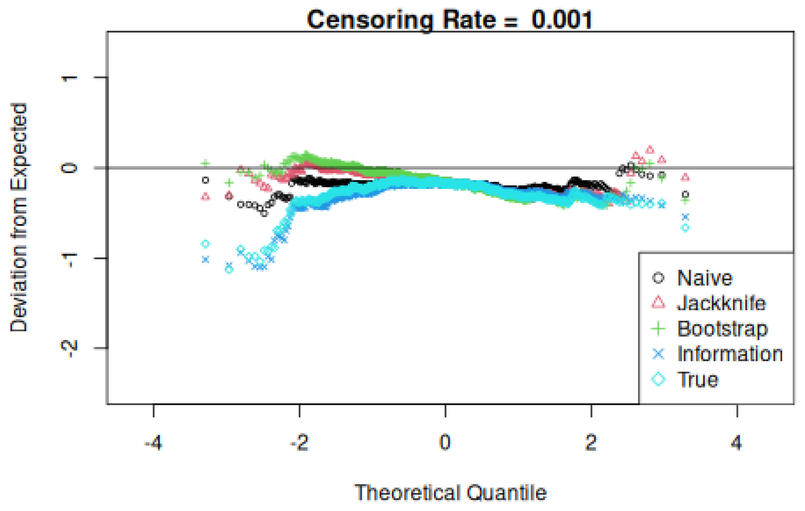
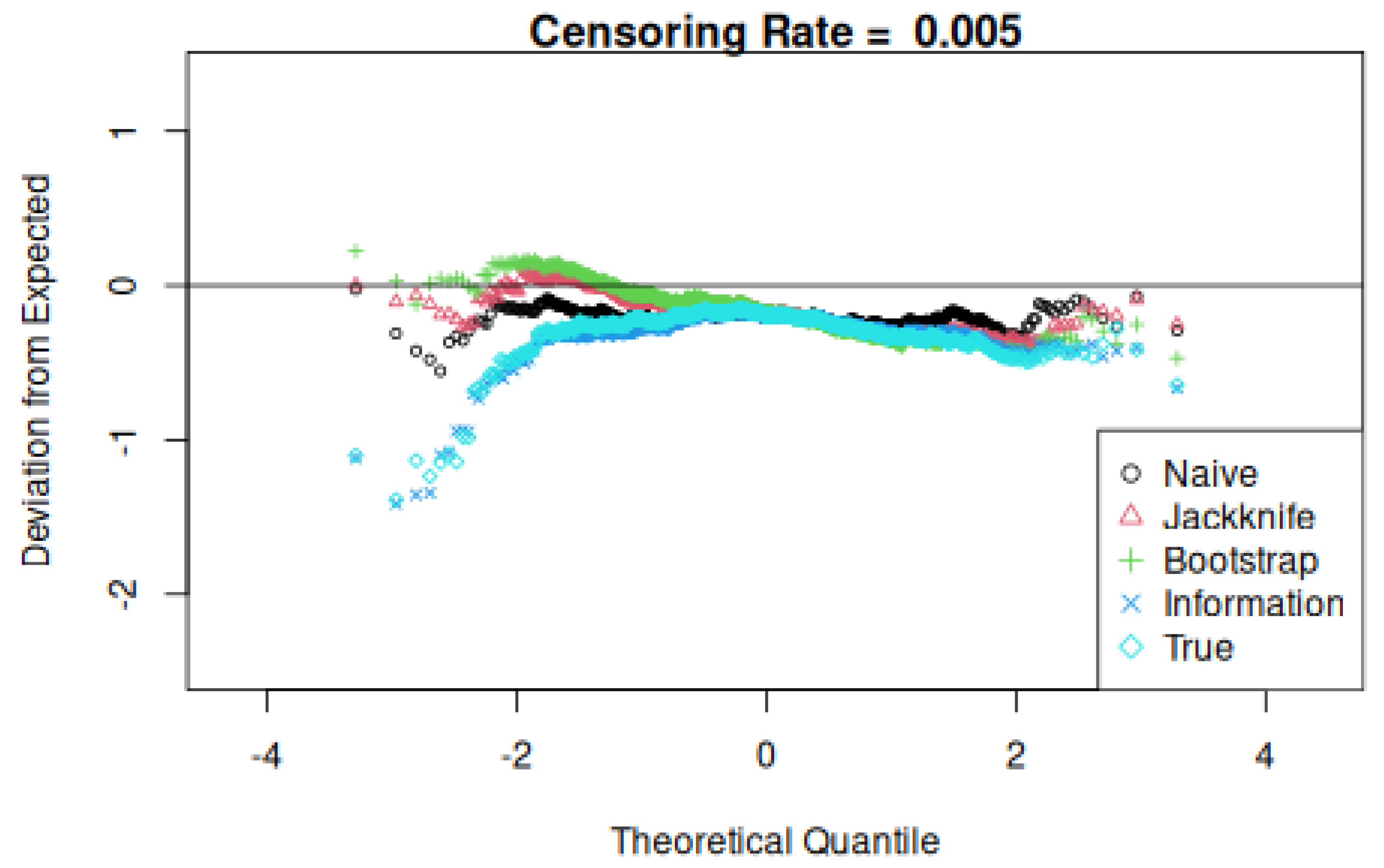
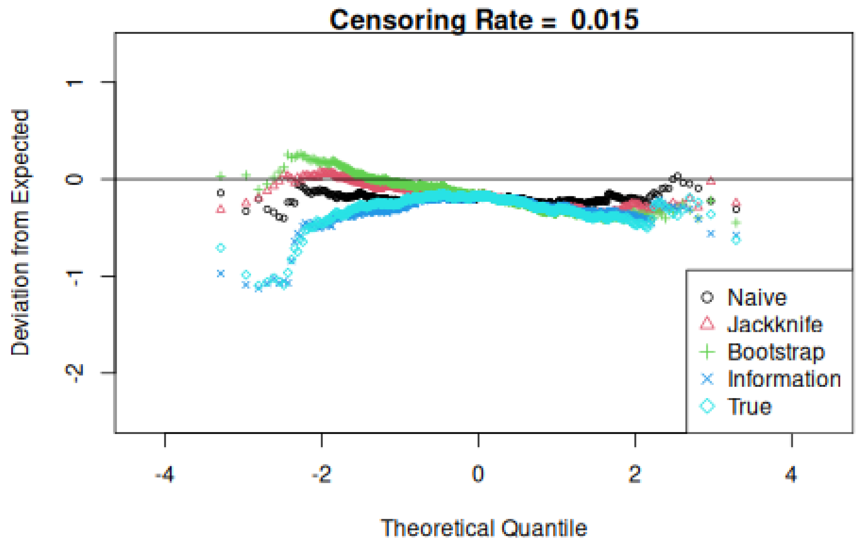
This research is motivated by the observation that likelihood-based inference provides p-values that are systematically too small; this was noted in the introduction and is manifest in the simulation below. A first step in determining the source of this discrepancy is to evaluate the quality of various standard errors.

Fix some constant k, and generate k data sets as per Section 2.1. For each simulated data set, several standard errors will be compared. These are as follows:

1.

The value calculated from the partial log-likelihood second derivative and referred to as the “naive” value;

2.

The value obtained from jackknifing and referred to as the “jackknife” value;

3.

The value obtained from the random-x bootstrap ([4]);

4.

The value determined from the expected second derivative of the log partial likelihood and referred to as the “information” value.

The computation of the first standard error value is relatively simple in standard Cox regression software as the second derivative of the partial likelihood evaluated at the parameter estimate. The next standard error is then given as a direct result of the jackknifing process.

The expectation (2) in the equation for the ideal standard error cannot be performed in closed form. In order to calculate the Fisher information, the following process is repeated K times. We wish to obtain the Fisher information, defined as in (2). Hence, each iteration generates a new set of time and status data, with fixed covariates. These simulated data are used to compute the average Fisher information, which is given by the second derivative of the partial log-likelihood $E\left({\ell }^{\prime \prime }\right)$. The square root of the inverse of this matrix is used as a standard error.

Three comparisons are then made, yielding tallied counts relative to the total k and counting the number of times that the true value exceeds naive, jackknife, and information values. Note that the true and information standard deviation value depend only on the covariate values and not on event and censoring times. Finally, plots of the difference between the theoretical and observed quantiles are made to assess their normality or lack thereof.

2.3. Considering the Continuity Correction

When a regressor in a Cox model takes integer values (for example, the covariates are indicator variables coding a categorical covariate), then potential values of the score statistic (i.e., the first derivative of the log partial likelihood associated with that covariate) have potential values in a discrete set, with values separated by one. That is, suppose that covariate i from model (2) takes on integer values, and let

$${\ell }^i={\displaystyle \frac{d}{d{\beta }_i}}\ell$$

(5)

be the components of the vector derivative used in (1). Then, potential values of the partial score ${\ell }^i$ are separated by one, and when using a normal approximation to calculate $P[{\ell }^i\ge {\ell }_{obs}^i]$ to obtain p-values, the profile likelihood ought to be modified by adjusting the data to reduce ${\ell }^j$ by one-half unit. Specifically, the score statistic is adjusted by adding $-\mathrm{sign}\left({\ell }^{\prime }\right)/2$ before multiplying by the inverse of the second derivative to obtain the next iteration in the profile likelihood maximization. This moves the partial score closer to its null hypothesis expectation. One might see this as a regression towards the mean; it might more directly be seen as the requirement to increase a p-value arising from a discrete distribution to include the entire probability atom reflecting the discrete observation.

This modification represents a continuity correction, and, to our knowledge, is newly presented in this manuscript in the context of proportional hazards regression.

As with more conventional regression models, if a sample of size n consists of covariate patterns drawn at random from a superpopulation, then standard errors for ${\ell }^j$ decrease at the rate of $n^{-1/2}$. A one-sided test of size $\alpha$ of a point null hypothesis that a parameter ${\beta }_j$ takes a value ${\beta }_j^0$ vs. the alternative that ${\beta }_j$ exceeds ${\beta }_j^0$ for the score test statistic ${\ell }^j$ is $\sqrt{I}{z}_{\alpha }$, for $z_{\alpha }$, the $1-\alpha$ quantile of a standard normal, and I is given by (2). Furthermore, $I=ni$, for i the Fisher information in a single observation, and hence the critical value for this one-sided test is $\sqrt{n}\sqrt{i}{z}_{\alpha }$. When the continuity correction is employed, the critical value becomes $\sqrt{n}\sqrt{i}{z}_{\alpha }+1/2$, and so the error in omitting the continuity correction is a multiple of $1/\sqrt{n}$.

Because normal approximations to Wald and the signed root of the likelihood ratio statistic are built around an approximate normality of the score, the data should be modified before applying normal approximations to these statistics as well. The p-values calculated for the Wald statistics are adjusted by comparing the root of (1) with the score redefined by adding $-\mathrm{sign}\left(l^{\prime }\right)/2$ to the score function. The resulting root is used in (3) and compared to a standard normal distribution.

We considered the effect of continuity correction on the behavior of the p-values. For the same k, we repeat the process from Section 2.1 a further k times. In each iteration, two Cox proportional hazards regressions are made: one with and one without a continuity correction. While the regression with no continuity correction is attained by maximizing the profile likelihood, the continuity correction requires the additional step of determining the numerical value of the adjustment itself.

Among these k Monte Carlo iterations, we report the proportion of data sets for which the two Cox proportional hazards models yield p-values satisfying $p<\alpha$ for $\alpha =0.01,0.05,0.10$. These results are tabulated in the next section.

3. Results

Figure 1, Figure 2, Figure 3 and Figure 4 represent the differences between the expected and empirical quantiles of estimates divided by the standard error associated with various standard error estimates for various censoring rates. That is, they are deviations of ordinates of the normal quantile from the ideal line with slope one and intercept zero.

Table 2. Proportions of p-values in various ranges without continuity correction.

$\mathit{\kappa }$	$\mathit{p}<0.01$	$\mathit{p}<0.05$	$\mathit{p}<0.10$
0.001	0.015	0.061	0.114
0.005	0.013	0.063	0.115
0.015	0.012	0.058	0.121
0.250	0.010	0.060	0.119

and

Table 3. Proportions of p-values in various ranges with continuity correction.

$\mathit{\kappa }$	$\mathit{p}<0.01$	$\mathit{p}<0.05$	$\mathit{p}<0.10$
0.001	0.010	0.053	0.102
0.005	0.012	0.058	0.102
0.015	0.008	0.052	0.109
0.250	0.009	0.052	0.105

represent frequency properties of the p-values for various censoring proportions with and without continuity correction. All are shown for simulated data sets consisting of 100 observations.

Note that the naive, jackknife, and bootstrap standard errors give similar patterns of deviation from normality. The true and simulated information standard deviations are similar to each other but at extreme parameter values show marked departures from normality; this is also reflected by large values for these standard errors in

Table 4. Skewness of Wald statistic values.

	Naive	Jackknife	Bootstrap	Information	True
0.001	−0.0429	0.0277	0.0505	−0.4082	−0.4224
0.005	−0.0180	0.0262	0.0555	−0.4508	−0.4780
0.015	0.0179	0.0277	0.0682	−0.3896	−0.4136
0.25	0.0256	0.0764	0.1135	−0.4213	−0.4625

and

Table 5. Excess kurtosis of Wald statistic values.

	Naive	Jackknife	Bootstrap	Information	True
0.001	0.2213	0.5453	0.4422	0.6040	0.7173
0.005	0.1217	0.3700	0.2745	0.7130	0.8917
0.015	0.0942	0.3289	0.2507	0.5441	0.7078
0.25	0.0786	0.3802	0.2257	0.5946	0.7723

.

4. Discussion

The quantile-quantile plots illustrate the observed standardized values subtracted from the expected quantile. From this, several conclusions can be made: first, the true Fisher information almost always underestimates the parameter standard deviation. Next, the naive partial likelihood method generally underestimates the true standard deviation, while the jackknife tends to overestimate it.

The plots depicting the same difference allows for comparison between the relative kurtosis of the different simulated standardizations. There appear to be patterns that are common to all four standardizations. The first such trend is the deviation from the expected theoretical quantile is typically negative, with a larger observed difference occurring at more negative theoretical quantiles. The converse holds true with positive theoretical quantiles having less negative differences, although at a smaller magnitude. Moreover, the inflection point of the graph occurs at 0. Both of these effects seem to be slightly magnified as $\kappa$ increases, with the final couple data points even slightly surpassing the theoretical quantile for the highest values of $\kappa$. The negative end at $\kappa =0.25$ drops off steeper, correspondingly. This all serves as an indication that the four approaches in order of increasing kurtosis are roughly (1) exact SD, (2) Fisher information, (3) jackknife, and (4) naive.

There are still some slight differences between the standardizations that can be seen across multiple values of $\kappa$. For example, jackknifing generally outperforms its naive counterpart, as expected. The negative ends of the plots also followed a similar relative order between the standardizations, albeit by small margins. For the most part, however, all four approaches have a similar performance. It should also be noted that the same observations held true for small sample sizes.

The coefficients of skewness and excess kurtosis for these standardized estimates were also calculated and are given in Table 4 and Table 5, respectively. The normal distribution has both of these values 0. By these measures, the naive standardization is superior.

For the next section of results, we examine the application of a continuity correction on the Cox regression. Table 2 and Table 3 report the frequency of how often $p<\alpha$ among the trials. These recorded frequencies correspond to the rate at which the simulated null hypotheses are rejected for various thresholds $\alpha$. When corresponding pairs fixing $\kappa$ and $\alpha$ are compared, it appears that the rate of rejection decreased and became closer to target values. This occurred in all instances, regardless of the actual value taken on by $\kappa$ or $\alpha$. Such a uniform change indicates an overall decrease in the anti-conservativeness of the Cox regression when a continuity correction is added to it.

Table 2 and Table 3 provide the most compelling evidence of the proposed correction’s effectiveness. In each case (see Table 2), the limit at the top represent the largest allowable probability of rejecting the null hypothesis. In most cases without the continuity correction, the probability of rejecting the null hypothesis rejects this threshold; in all cases with continuity correction (see Table 3), the probability of incorrectly rejecting the null hypothesis is almost exactly the target value. We thank the referee for this suggestion.

4.1. An Example

Consider the data set reflecting the survival of 23 subjects with acute myelogenous leukemia (AML) provided by [8] and distributed by [9]. The data consist of times, censoring status, and a dichotomous covariate. The Gaussian approximation to the p-values for the bivariate covariates are 0.0737 and 0.124 without and with continuity correction, respectively. The simulation results above indicate that the continuity-corrected value is more reliable. This difference is large enough to be important.

The naive and jackknife standard errors are 0.5119 and 0.5051, respectively. This difference is less striking but still large enough to attract attention.

4.2. A Second Example

Consider the example of [10] containing information on 100 breast cancer patients, including survival time, survival status, tumor stage, nodal status, grading, and cathepsin-D expression. Tumor stage, nodal status, and cathepsin-D expression are all dichotomous, and so the continuity correction as above is appropriate.

Table 6. Breast cancer results without continuity correction.

Effect	Estimate	Standard Error	p-Value
T	1.5604	0.5013	0.00185
N	1.1342	0.4323	0.00870
CD	0.5207	0.4496	0.24680

and

Table 7. Breast cancer results with continuity correction.

Effect	Estimate	Standard Error	p-Value
T	1.4375	0.4906	0.00339
N	1.1353	0.4292	0.00817
CD	0.5584	0.4479	0.21250

show the results of fitting this model without and with continuity correction, respectively. Table 7 is only interesting for its p-values; these are larger than those of Table 6, and as demonstrated in Table 2 and Table 3, the resulting sizes of tests without continuity correction are incorrectly inflated.

Here, the naive standard error for tumor stage is 0.501, and the jackknife estimate is 0.533. The bootstrap estimate at 1.363 behaves poorly, since the bootstrap samples include cases in which the parameter estimate is effectively infinite.

5. Conclusions

Overall, the four discussed standard error calculations for a Cox proportional hazards model exhibit the following behaviors: Fisher information and naive partial likelihood methods tend to underestimate the true standard deviation, while jackknifing over-corrects with an overestimation. After considering the difference between the theoretical and observed quantiles, it was found that, in order of increasing kurtosis, the standardizations are generally (1) exact SD, (2) Fisher information, (3) jackknife, and (4) naive. Finally, adding a continuity correction to the model adequately reduces the anti-conservativeness that would be observed without one.

References

1. Cox, D.; Hinkley, D. Theoretical Statistics; Chapman and Hall: Boca Raton, MA, USA, 1974. [Google Scholar]
2. Casella, G.; Berger, R.L. Statitical Inference; Duxbury: Pacific Grove, CA, USA, 2002. [Google Scholar]
3. Quenouille, M.H. Notes on Bias in Estimation. Biometrika 1956, 43, 353–360. [Google Scholar] [CrossRef]
4. Efron, B.; Tibshirani, R. Bootstrap Methods for Standard Errors, Confidence Intervals, and Other Measures of Statistical Accuracy. Stat. Sci. 1986, 1, 54–75. [Google Scholar] [CrossRef]
5. Cox, D.R. Regression Models and Life-Tables. J. R. Stat. Soc. Ser. B (Methodol.) 1972, 34, 187–202. [Google Scholar] [CrossRef]
6. Kleinbaum, D.G. Survival Analysis; Springer: New York, NY, USA, 1996. [Google Scholar] [CrossRef]
7. Andersen, P.K.; Gill, R.D. Cox’s Regression Model for Counting Processes: A Large Sample Study. Ann. Stat. 1982, 10, 1100–1120. [Google Scholar] [CrossRef]
8. Miller, R.G. Survival Analysis; John Wiley and Sons: Hoboken, NJ, USA, 1997. [Google Scholar]
9. Therneau, T.M. A Package for Survival Analysis in R; R Package Version 3.5-8. Comprehensive R Archive Network. 2024. Available online: https://CRAN.R-project.org/package=survival (accessed on 2 May 2025).
10. Heinze, G.; Schemper, M. A Solution to the Problem of Monotone Likelihood in Cox Regression. Biometrics 2001, 57, 114–119. [Google Scholar] [CrossRef] [PubMed]
Figure 1. Wald statistic transformed quantiles with κ = 0.001.
Stats 08 00061 g001
Figure 2. Wald statistic transformed quantiles with κ = 0.005.
Stats 08 00061 g002
Figure 3. Wald statistic transformed quantiles with κ = 0.015.
Stats 08 00061 g003
Figure 4. Wald statistic transformed quantiles with κ = 0.25.
Stats 08 00061 g004