Some Useful Techniques for High-Dimensional Statistics

Abstract

High-dimensional statistics are used when $n<5p$, where n is the sample size and p is the number of predictors. Useful techniques include (a) the use of a sparse fitted model, (b) use of principal component analysis for dimension reduction, (c) use of alternative multivariate dispersion estimators instead of the sample covariance matrix, (d) eliminate weak predictors, and (e) stack low-dimensional estimators into a vector. Some variants and theory for these techniques will be given or reviewed.

1. Introduction

High-dimensional statistics are used when $n<5p$, where n is the sample size and p is the number of variables. Such a model is overfitting: the model does not have enough data to estimate the p parameters accurately. Then n tends to not be large enough for the classical statistical method to be useful. An alternative (but less general) definition of high-dimensional statistics is that p is large. Sometimes $p>Kn$ with $K\ge 10$ is called ultrahigh-dimensional statistics.

Some important statistical methods include regression, multivariate statistics, and classification. These methods are important for statistical learning ≈ machine learning, an important part of artificial intelligence. Let predictor variables for regression or multivariate statistics be $\mathit{x}={(x_1,\dots ,x_p)}^T.$ Let Y be a response variable for regression or classification. Important regression models include generalized linear models, nonlinear regression, nonparametric regression, and survival regression models. Inference for multivariate regression where there are m response variables $Y_1,\dots ,Y_m$ is also of interest. Useful references for the following statistical methods include [1,2,3].

Let the population covariance matrices

$$\mathrm{Cov}\left(\mathit{x}\right)=E\left[(\mathit{x}-E\left(\mathit{x}\right)){(\mathit{x}-E\left(\mathit{x}\right))}^T\right]={\mathbf{\Sigma }}_{\mathit{x}},\mathrm{and}$$

$$\mathrm{Cov}(\mathit{x},Y)=E\left[(\mathit{x}-E\left(\mathit{x}\right))(Y-E\left(Y\right))\right]={\mathbf{\Sigma }}_{\mathit{x}Y}.$$

Let the sample covariance matrices be

$${\widehat{\mathbf{\Sigma }}}_{\mathit{x}}={\displaystyle \frac{1}{n-1}}\sum _{i=1}^n({\mathit{x}}_i-\overline{\mathit{x}}){({\mathit{x}}_i-\overline{\mathit{x}})}^T\mathrm{and}{\widehat{\mathbf{\Sigma }}}_{\mathit{x}Y}={\displaystyle \frac{1}{n-1}}\sum _{i=1}^n({\mathit{x}}_i-\overline{\mathit{x}})(Y_i-\overline{Y}).$$

Let the population correlation ${\rho }_{ij}={\rho }_{x_i,x_j}=\mathrm{Cor}(x_i,x_j)$ and the sample correlation $r_{ij}=r_{x_i,x_j}=\mathrm{cor}(x_i,x_j).$ Let the population correlation matrices $\mathrm{Cor}\left(\mathit{x}\right)={\mathsf{\rho }}_{\mathit{x}}=\left({\rho }_{ij}\right)$ and $\mathrm{Cor}(\mathit{x},Y)={\mathsf{\rho }}_{\mathit{x}Y}={({\rho }_{x_1,Y},\dots ,{\rho }_{x_p,Y})}^T.$ Let the sample covariance matrices be ${\mathit{R}}_{\mathit{x}}=\left(r_{ij}\right)$ and ${\mathit{r}}_{\mathit{x}Y}={(r_{{\mathit{x}}_1,Y},\dots ,r_{{\mathit{x}}_p,Y})}^T.$ Then ${\widehat{\mathbf{\Sigma }}}_{\mathit{x}}$ and R are dispersion estimators, and $(\overline{\mathit{x}},{\widehat{\mathbf{\Sigma }}}_{\mathit{x}})$ is an estimator of multivariate location and dispersion.

Suppose the positive semi-definite dispersion matrix $\mathbf{\Sigma }$ has eigenvalue eigenvector pairs $({\lambda }_1,{\mathit{d}}_1),\dots ,({\lambda }_p,{\mathit{d}}_p)$, where ${\lambda }_1\ge {\lambda }_2\ge \cdots \ge {\lambda }_p$. Let the eigenvalue eigenvector pairs of $\widehat{\mathbf{\Sigma }}$ be $({\widehat{\lambda }}_1,{\widehat{\mathit{d}}}_1),\dots ,({\widehat{\lambda }}_p,{\widehat{\mathit{d}}}_p)$, where ${\widehat{\lambda }}_1\ge {\widehat{\lambda }}_2\ge \cdots \ge {\widehat{\lambda }}_p$. These vectors are important quantities for principal component analysis (PCA).

Let the multiple linear regression model

$$Y_i=\alpha +x_{i,1}{\beta }_1+\cdots +x_{i,p}{\beta }_p+e_i=\alpha +{\mathit{x}}_i^T\mathsf{\beta }+e_i$$

(1)

for $i=1,\dots ,n.$ In matrix form, this model is $\mathit{Y}=\mathit{X}\mathsf{\delta }+\mathit{e}$, where Y is an $n\times 1$ vector of dependent variables, X is an $n\times (p+1)$ matrix of predictors, $\mathsf{\delta }={(\alpha ,{\mathsf{\beta }}^T)}^T$ is a $(p+1)\times 1$ vector of unknown coefficients, and e is an $n\times 1$ vector of unknown errors. Assume that the $e_i$ are independent and identically distributed (iid) with expected value $E\left(e_i\right)=0$ and variance $V\left(e_i\right)={\sigma }^2.$

Principal components regression (PCR), partial least squares (PLS), and several other dimension reduction models use p linear combinations ${\mathit{\gamma }}_1^T\mathit{x},\dots ,{\mathit{\gamma }}_p^T\mathit{x}$. Estimating the ${\mathit{\gamma }}_i$ and performing the ordinary least squares (OLS) regression of Y on $({\widehat{\mathit{\gamma }}}_1^T\mathit{x},{\widehat{\mathit{\gamma }}}_2^T\mathit{x},\dots ,{\widehat{\mathit{\gamma }}}_k^T\mathit{x})$ and a constant gives the k-component estimator, e.g., the k-component PLS estimator or the k-component PCR estimator, for $k=1,\dots ,J$ where $J\le p$ and the p-component estimator is the OLS estimator ${\widehat{\mathsf{\beta }}}_{OLS}$. Let ${\mathit{\gamma }}_i\left(PCR\right)={\mathit{d}}_i$ and ${\mathit{\gamma }}_i={\mathit{\gamma }}_i\left(PLS\right).$ The model selection estimator chooses one of the k-component estimators, e.g., using cross validation, and it will be denoted by ${\widehat{\mathsf{\beta }}}_{MSPLS}$ or ${\widehat{\mathsf{\beta }}}_{MSPCR}$.

Let $\mathit{X}=\left[\mathbf{1}{\mathit{X}}_1\right]$. Ref.  [4] noted that one way to formulate PLS is to solve an optimization problem by forming ${\mathit{b}}_j={\widehat{\mathit{\gamma }}}_j$ iteratively where

$${\mathit{b}}_k=arg\underset{\mathit{b}}{max}\left\{{\left[\mathrm{Cor}(\mathit{Y},{\mathit{X}}_1\mathit{b})\right]}^{2}V\left({\mathit{X}}_1\mathit{b}\right)\right\}$$

(2)

subject to ${\mathit{b}}^T\mathit{b}=1$ and ${\mathit{b}}^T{\mathbf{\Sigma }}_{\mathit{x}}{\mathit{b}}_j=0$ for $j=1,\dots ,k-1.$ Here V stands for the variance. So PLS is a model free way to get predictors ${\widehat{\mathit{\gamma }}}_i^T\mathit{x}$ that are fairly highly correlated with the response, and the absolute correlations tend to decrease quickly.

In high dimensions, it is very difficult to estimate a $p\times 1$ vector $\mathsf{\theta }$, e.g., $\mathsf{\theta }=\mathsf{\beta }$ or $\mathsf{\theta }={\mathbf{\Sigma }}_{\mathit{x}Y}$. This result is a form of “the curse of dimensionality”. If a $\sqrt{n}$ consistent estimator of $\mathsf{\theta }$ is available, then the squared norm

$$\parallel \widehat{\mathsf{\theta }}{-\mathsf{\theta }\parallel }^2=\sum _{i=1}^p{({\widehat{\theta }}_i-{\theta }_i)}^2\propto p/n.$$

(3)

Since $\widehat{\mathsf{\theta }}$ is a consistent estimator of $\mathsf{\theta }$ if $\parallel \widehat{\mathsf{\theta }}{-\mathsf{\theta }\parallel }^2\to 0$ as $n\to \infty$, often the high-dimensional estimator $\widehat{\mathsf{\theta }}$ has not shown to be consistent, except under very strong regularity conditions.

Although this paper reviews some important techniques for high-dimensional statistics, there is also new material. First, for multiple linear regression, Section 2.1 proves that “sensible model selection estimators” produce fitted values similar to that of the full OLS model when n is much larger than p, even if heterogeneity is present. Second, Section 2.3 shows how to improve PCR and gives a new explanation for why PLS components should be used instead of PCR components from PCA. Third, Section 2.3 provides a relationship between canonical correlation analysis and PLS. Fourth, Section 2.3 introduces the SC scree plot. Fifth, Section 2.5 suggests a simple method for choosing $\delta$ for a regularized correlation matrix ${\mathit{R}}_{\delta }$. The outlier-resistant methods of Section 2.5 are not new, but they have never been used for most high-dimensional procedures.

2. Materials and Methods

2.1. Model Selection Estimators in Low Dimensions

This subsection explains why “sensible model selection estimators, including variable selection estimators,” produce fitted values (predictions) similar to that of the full OLS model when n is much larger than p. The result in Equation (4) that the residuals from the model selection model and the full OLS model are highly correlated was a property of OLS and Mallow’s $C_p$ criterion, not of any underlying model, but linearity forces the fitted values to be highly correlated. Hence the result works if OLS is consistent and the population model is linear, so for weighted least squares, AR(p) time series, serially correlated errors, et cetera. In particular, the cases do not need to be iid from some distribution. Since the correlation gets arbitrarily close to 1, the model selection estimator and full OLS estimator are estimating the same population parameter $\mathsf{\beta }$, but it is possible that the model selection estimator picks the full OLS model with probability going to one.

Consider the OLS regression of Y on a constant and $\mathit{w}={(W_1,\dots ,W_p)}^T$ where, for example, $W_j=x_j$, $W_j={\widehat{\mathit{\gamma }}}_j^T\mathit{x}$, or $W_j={\widehat{\mathit{d}}}_j^T\mathit{x}$. Let I index the variables in the model so $I=\{1,2,4\}$ means that ${\mathit{w}}_I={(W_1,W_2,W_4)}^T$ was selected. The full model $I=F$ uses all p predictors and the constant with ${\mathsf{\beta }}_I={\mathsf{\beta }}_F=\mathsf{\beta }={\mathsf{\beta }}_{OLS}$. Let r be the residuals from the full OLS model and let $r_I$ be the residuals from model I that uses ${\widehat{\mathsf{\beta }}}_I$. Suppose model I uses k predictors including a constant with $2\le k\le p+1$. Ref.  [5] proved that the model I with k predictors that minimizes [6] $C_p\left(I\right)$ maximizes cor($r,r_I)$, that

$$\mathrm{cor}(r,r_I)=\sqrt{{\displaystyle \frac{n-(p+1)}{C_p\left(I\right)+n-2k}}},$$

and under linearity, cor($r,r_I)\to 1$ forces

$$cor(\widehat{\alpha }+{\mathit{w}}^T\widehat{\mathsf{\beta }},{\widehat{\alpha }}_I+{\mathit{w}}_I^T{\widehat{\mathsf{\beta }}}_I)=\mathrm{cor}(\mathrm{ESP},\mathrm{ESP}\left(\mathrm{I}\right))=\mathrm{cor}(\widehat{\mathrm{Y}},{\widehat{\mathrm{Y}}}_{\mathrm{I}})\to 1.$$

Thus $C_p\left(I\right)\le 2k$ implies that

$$\mathrm{cor}(\mathrm{r},{\mathrm{r}}_{\mathrm{I}})\ge \sqrt{1-{\displaystyle \frac{\mathrm{p}+1}{\mathrm{n}}}}.$$

(4)

Let the model $I_{min}$ minimize the $C_p$ criterion among the models considered with $C_p\left(I\right)\le 2k_I$. Then $C_p\left(I_{min}\right)\le C_p\left(F\right)=p+1$, and if PLS or PCR is selected using model selection (on models $I_1,\dots ,I_p$ with $I_j=\{1,2,\dots ,j\}$ corresponding to the j-component regression) with the $C_p\left(I\right)$ criterion, and $n\ge 20(p+1)$, then cor($r,r_I)\ge \sqrt{19/20}=0.974.$ Hence the correlation of ESP(I) and ESP(F) will typically also be high. (For PCR, the following variant should work better, as follows: take $U_j={\widehat{\mathit{d}}}_j^T\mathit{x}$ and $W_1$ as the $U_j$ with the highest squared correlation with Y, $W_2$ as the $U_j$ with the second highest squared correlation, etc.).

Machine learning methods for the multiple linear regression model can be incorporated as follows. Let k be the number of predictors selected by lasso, including a constant. Standardize the predictors to have unit sample variance and run the method. Let model I contain the variables corresponding to the $k-1$ predictors variables that have the largest $|{\widehat{\beta }}_i|$. Fit the OLS model I to these predictors and a constant. If $C_p\left(I\right)<min(2k,p+1)$, use model I; otherwise, use the full OLS model. Many variants are possible. In low dimensions, comparisons between methods like lasso, PCR, PLS, and envelopes might use prediction intervals, the amount of dimension reduction, and standard errors if available.

If the above procedure is used, then model selection estimators, such as ${\widehat{\mathsf{\beta }}}_{MSPLS}$, produce predictions that are similar to those of the OLS full model if $n\ge 20(p+1)$. Other model selection criterion, such as k-fold cross validation, tend to behave like $C_p$ in low dimensions, but getting bounds like Equation (4) may be difficult. Empirically, variable selection estimators and model selection estimators often do not select the full model. Equation (4) suggests that “weak” predictors will often be omitted, as long as cor($r,r_I)$ stays high. (If the predictors are not orthogonal, “weak” might mean the predictor is not very useful given that the other predictors are in the model).

It is common in the model selection literature to assume, for the full model, that there is a model S such that ${\beta }_i\ne 0$ for $i\in S$, and ${\beta }_i=0$ for $i\notin S$. Then model I underfits unless $S\subseteq I$. If $S⊈I$, then an “important” predictor has been left out of the model. Then under the model ${\mathit{x}}^T\mathsf{\beta }={\mathit{x}}_S^T{\mathsf{\beta }}_S$, $\mathrm{cor}(r,r_I)$ will not converge to 1 as $n\to \infty$, and for large enough n, ${\left[\mathrm{cor}(r,r_I)\right]}^2\le \gamma <1$. Thus $C_p\left(I\right)\to \infty$ as $n\to \infty$. Hence $P(S\subseteq I_{min})\to 1$ as $n\to \infty$ where $I_{min}$ corresponds to the set of predictors selected by a variable selection method such as forward selection or lasso variable selection. Thus the probability that the model selection estimator underfits goes to zero as $n\to \infty$ if p is fixed, the full model is one of the models considered, and the $C_p$ criterion is used, as noted by [7].

For real data, an important question in variable selection is whether ${\beta }_i=0$ is a reasonable assumption. If X has full rank $p+1$, then having ${\beta }_i$ equal to zero for 20 decimal places may not be reasonable. See, for example, [8,9,10]. Then the probability that the variable selection estimator chooses the full model goes to one if the probability of underfitting goes to 0 as $n\to \infty$. If ${\widehat{\mathsf{\beta }}}_I$ is $a\times 1$, use zero padding to form the $p\times 1$ vector ${\widehat{\mathsf{\beta }}}_{I,0}$ from ${\widehat{\mathsf{\beta }}}_I$ by adding 0s corresponding to the omitted variables.

For example, if $p=3$ and $Y=\alpha +{\mathit{x}}_1+0{\mathit{x}}_2+0{\mathit{x}}_3+e$, then $S=\left\{1\right\}$ and ${\mathsf{\beta }}_{S,0}={(1,0,0)}^T=\mathsf{\beta }={({\beta }_1,{\beta }_2,{\beta }_3)}^T={\mathsf{\beta }}_F.$ This population model has $a=a_S=1$ active predictors. Then the $J=2^p=8$ possible subsets of $F=\{1,2,\dots ,p\}$ are $I_1=\varnothing$, $S=I_2=\left\{1\right\}$, $I_3=\left\{2\right\}$, $I_4=\left\{3\right\}$, $I_5=\{1,2\}$, $I_6=\{1,3\}$, $I_7=\{2,3\}$, and $F=I_8=\{1,2,3\}$. There are $2^{p-a_S}=4$ subsets $I_2,I_5,I_6,$ and $I_8$ such that $S\subseteq I_j$. Let ${\widehat{\mathsf{\beta }}}_{I_7}={({\widehat{\beta }}_2,{\widehat{\beta }}_3)}^T$ and ${\mathit{x}}_{I_7}={(x_2,x_3)}^T.$ If ${\widehat{\mathsf{\beta }}}_{I_{min}}={({\widehat{\beta }}_1,{\widehat{\beta }}_3)}^T$, then the observed variable selection estimator ${\widehat{\mathsf{\beta }}}_{VS}={\widehat{\mathsf{\beta }}}_{I_{min},0}={({\widehat{\beta }}_1,0,{\widehat{\beta }}_3)}^T.$ As a statistic, ${\widehat{\mathsf{\beta }}}_{VS}={\widehat{\mathsf{\beta }}}_{I_k,0}$ with probabilities ${\pi }_{kn}=P(I_{min}=I_k)$ for $k=1,\dots ,J$ where there are J subsets, e.g., $J=2^p-1$. Theory for the variable selection estimator ${\widehat{\mathsf{\beta }}}_{VS}$ is complicated. See [7] for models such as multiple linear regression, GLMs, and [11] Cox proportional hazards regression.

2.2. Sparse Fitted Models

A fitted or population regression model is sparse if a of the predictors are active (have nonzero ${\widehat{\beta }}_i$ or ${\beta }_i$) where $n\ge Ja$ with $J\ge 10$. Otherwise, the model is nonsparse. A high-dimensional population full regression model is abundant or dense if the regression information is spread out among the p predictors (nearly all of the predictors are active). Hence an abundant model is a nonsparse model. Under the above definitions, most classical low-dimensional models use sparse fitted models, and statisticians have over one hundred years of experience with such models.

The literature for high-dimensional sparse regression models often assumes that (i) ${\mathsf{\beta }}_{I,0}=\mathsf{\beta }={\mathsf{\beta }}_F$, that (ii) $S\subseteq I$ where I uses k predictors including a constant, and that (iii) $n\ge 10k$. When these assumptions hold, the population model is sparse, the fitted model is sparse, and Equation (3) becomes $\parallel {\widehat{\mathsf{\beta }}}_{I,0}{-\mathsf{\beta }\parallel }^2$, which can be small. Getting rid of assumption (i) and the assumption that $S\subseteq I$ greatly increases the applicability of variable selection estimators, such as forward selection, lasso, and the elastic net, for high-dimensional data, even if $\parallel {\widehat{\mathsf{\beta }}}_{I,0}{-\mathsf{\beta }\parallel }^2$ is huge. As argued in the following paragraphs, the sparse fitted model often fits the data well, and often ${\widehat{\mathsf{\beta }}}_I$ is a good estimator of ${\mathsf{\beta }}_I$.

A sparse fitted model transforms a high-dimensional problem into a low-dimensional problem, and the sparse fitted model can be checked with the goodness of fit diagnostics available for that low-dimensional model. If the predictors used by the sparse fitted regression model are ${\mathit{x}}_I$, and if the regression model depends on ${\mathit{x}}_I$ only through the sufficient predictor $SP={\alpha }_I+{\mathit{x}}_I^T{\mathsf{\beta }}_I$, then a useful diagnostic is the response plot of $ESP\left(I\right)={\widehat{\alpha }}_I+{\mathit{x}}_I^T{\widehat{\mathsf{\beta }}}_I$ versus the response Y on the vertical axis. If there is goodness of fit, then ${\widehat{\mathsf{\beta }}}_I$ tends to estimate ${\mathsf{\beta }}_I$ regardless of whether the population model is sparse or nonsparse. Data splitting may be needed for valid inference such as hypothesis testing.

Suppose the cases ${({\mathit{x}}_i^T,Y_i)}^T$ are iid for $i=1,\dots ,n$. Then $Y_1,\dots ,Y_n$ are iid, resulting in a valid sparse fitted model regardless of whether the population model is sparse or nonsparse. This null model omits all of the predictors. For high-dimensional data, a reasonable goal is to find a model that greatly outperforms the null model.

The sparse fitted model using $(Y,{\mathit{x}}_I)$ is often useful when there are one or more strong predictors. The following [12] theorem gives two more situations where a sparse fitted model can greatly outperform the null model. The population models in Theorem 1 can be sparse or nonsparse. The high-dimensional multiple linear regression literature often assumes that the cases are iid from a multivariate normal distribution, and that the population model is sparse. Let ${\Sigma }_Y={\sigma }_Y^2$. For multiple linear regression, note that ${\sigma }_O^2<{\sigma }_Y^2={\Sigma }_Y$ unless ${\mathsf{\eta }}^T{\mathbf{\Sigma }}_{\mathit{x}Y}=0$.

Theorem 1.

Suppose the cases ${(Y_i,{\mathit{x}}_i^T)}^T$ are iid from some distribution.

(a) If the joint distribution of ${(Y,{\mathit{x}}^T)}^T$ is multivariate normal,

$$\left(\begin{array}{c}Y\\ \mathit{x}\end{array}\right)\sim N_{p+1}\left(\begin{array}{cc}\left(\begin{array}{c}{\mu }_Y\\ {\mathsf{\mu }}_{\mathit{x}}\end{array}\right),& \left(\begin{array}{cc}{\Sigma }_Y& {\mathbf{\Sigma }}_{Y\mathit{x}}\\ {\mathbf{\Sigma }}_{\mathit{x}Y}& {\mathbf{\Sigma }}_{\mathit{x}}\end{array}\right)\end{array}\right),$$

then $Y|\mathit{x}\sim Y|({\alpha }_{OLS}+{\mathsf{\beta }}_{OLS}^T\mathit{x})\sim N({\alpha }_{OLS}+{\mathsf{\beta }}_{OLS}^T\mathit{x},{\sigma }^2)$ follows a multiple linear regression model, but so does $Y|{\mathsf{\eta }}^T\mathit{x}\sim N({\alpha }_O+{\mathsf{\beta }}_O^T\mathit{x},{\sigma }_O^2)$, where ${\alpha }_O={\mu }_Y-{\mathsf{\beta }}_O^T{\mathsf{\mu }}_{\mathit{x}}$, ${\mathsf{\beta }}_O=\lambda \mathsf{\eta }$, ${\sigma }_O^2={\Sigma }_Y-{\mathsf{\beta }}_O^T{\mathbf{\Sigma }}_{\mathit{x}Y},$ and

$$\lambda ={\displaystyle \frac{{\mathbf{\Sigma }}_{\mathit{x}Y}^T\mathsf{\eta }}{{\mathsf{\eta }}^T{\mathbf{\Sigma }}_{\mathit{x}}\mathsf{\eta }}}.$$

(b) If the response Y is binary, then $Y\left|\right({\alpha }_O+{\mathsf{\beta }}_O^T\mathit{x})\sim$ binomial($m=1,\rho ({\alpha }_O+{\mathsf{\beta }}_O^T\mathit{x}))$ where $E\left[Y\right|({\alpha }_O+{\mathsf{\beta }}_O^T\mathit{x})]=\rho ({\alpha }_O+{\mathsf{\beta }}_O^T\mathit{x})=P[Y=1|({\alpha }_O+{\mathsf{\beta }}_O^T\mathit{x})]$. Hence every linear combination of the predictors satisfies a binary regression model.

2.3. PCA-PLS

Another technique is to use PCA for dimension reduction. Let $U_1,\dots ,U_p$ be the PCA linear combinations ($U_i={\widehat{\mathit{\gamma }}}_i^T\mathit{x}$) ordered with respect to the largest eigenvalues. Then use $U_1,\dots ,U_k$ in the regression or classification model where k is chosen in some manner. This method can be used for models with m response variables $Y_1,\dots ,Y_m$. See, for example, [13,14,15,16].

Consider a low or high-dimensional regression or classification method with a univariate response variable Y. Let $W_1,\dots ,W_p$ be the linear combinations ordered with respect to the highest squared correlations $r_1^2\ge r_2^2\ge \cdots \ge r_p^2$ where the sample correlation $r_{i,Y}=\mathrm{cor}({\mathit{x}}_i,Y)$. From a model selection viewpoint, using $W_1,\dots ,W_k$ should work much better than using $U_1,\dots ,U_k$. Also, the PLS components $W_i$ should be used instead of the PCA $W_i$, since the PLS components are chosen to be fairly highly correlated with Y. See Equation (2). Ref.  [17] (pp. 71–72) shows that an equivalent way to compute the k-component PLS estimator is to maximize ${\widehat{\mathit{\gamma }}}^T{\widehat{\mathbf{\Sigma }}}_{\mathit{x}Y}$ under some constraints. If the predictors are standardized to have unit sample variance, then this method becomes a correlation vector optimization problem. Ref.  [18] use the PLS components as predictors for nonlinear regression, but the above model selection viewpoint is new.

From canonical correlation analysis (CCA), if ${(Y_i,{\mathit{x}}_i^T)}^T$ are iid, then

$$M=\underset{\mathit{\gamma }\ne \mathbf{0}}{max}\mathrm{Cor}({\mathit{\gamma }}^T\mathit{x},Y)=\underset{\mathit{\gamma }\ne \mathbf{0}}{max}{\displaystyle \frac{{\mathit{\gamma }}^T{\mathbf{\Sigma }}_{\mathit{x}Y}}{\sqrt{{\Sigma }_Y}\sqrt{{\mathit{\gamma }}^T{\mathbf{\Sigma }}_{\mathit{x}}\mathit{\gamma }}}}.$$

This optimization problem is equivalent to maximizing

$${\mathbf{\Sigma }}_Y{M}^2=\underset{\mathit{\gamma }\ne 0}{max}{\displaystyle \frac{{\mathit{\gamma }}^T{\mathbf{\Sigma }}_{\mathit{x}Y}{\mathbf{\Sigma }}_{\mathit{x}Y}^T\mathit{\gamma }}{{\mathit{\gamma }}^T{\mathbf{\Sigma }}_{\mathit{x}}\mathit{\gamma }}},$$

which has a maximum at $\mathit{\gamma }={\mathbf{\Sigma }}_{\mathit{x}}^{-1}{\mathbf{\Sigma }}_{\mathit{x}Y}={\mathsf{\beta }}_{OLS}.$ See [19] (pp. 168, 282). Hence PLS is a lot like CCA for ${(Y_i,{\mathit{x}}_i^T)}^T$ but with more constraints, and PLS can be computed in high dimensions. From the dimension reduction literature, if Y depends on x only through $\alpha +{\mathsf{\beta }}^T\mathit{x}$, then under the assumption of “linearly related predictors,” ${\widehat{\mathsf{\beta }}}_{OLS}$ estimates ${\mathsf{\beta }}_{OLS}=c\mathsf{\beta }$ for some constant c which is often nonzero. See, for example, [20] (p. 432).

The above results suggest computing lasso for multiple linear regression, find the number of predictors k chosen by lasso, and take k linear combinations $W_i$. An SC scree plot of i versus $r_i^2$ behaves like a scree plot of i versus the eigenvalues. Hence quantities like ${\sum }_{i=1}^j{r}_i^2/{\sum }_{i=1}^p{r}_i^2$ are of interest for $j=1,\dots ,p$, and scree plot techniques could be adapted to choose k. Many other possibilities exist, and there are many possibilities for models with m response variables $Y_1,\dots ,Y_m$. See [18] for some ideas.

Another useful technique is to eliminate weak predictors before finding $W_1,\dots ,W_k$. By Equation (3), ${\widehat{\mathit{\gamma }}}_i$ may not be close to ${\mathit{\gamma }}_i$ in high dimensions, e.g., $p=n^6$. For example, the sample eigenvectors ${\widehat{\mathit{d}}}_i$ tend to be poor estimators of the population eigenvectors ${\mathit{d}}_i$ of ${\mathbf{\Sigma }}_{\mathit{x}}$. An exception is when the correlation Cor$(x_i,x_j)=\rho$ for $i\ne j$ where $\rho$ is close to 1. See [21]. One possibility is to take the j predictors $x_i$ with the highest squared correlations with Y. The SC scree plot is useful. Then do lasso (meant for the multiple linear regression model) to further reduce the number of $x_i$. Here j should be proportional to n, for example, $j=min(Kn,p)$, where $K=1$ is an interesting choice. When n is small, spurious correlations can be a problem as follows: if the actual correlation is near 0, the sample size n may need to be large before the sample correlation $r_i$ is near 0. For more on the importance of eliminating weak predictors and high-dimensional variable selection, see, for example, [22,23,24,25,26].

2.4. Stack Low-Dimensional Estimators into a Vector

Another technique is to stack low-dimensional estimators into a vector. For example ${\overline{\mathit{x}}}_2-{\overline{\mathit{x}}}_1$, and elements from an estimated covariance matrix such as $\mathit{c}=vech\left({\mathbf{\Sigma }}_{\mathit{z}}\right)$. Using $\mathit{z}={(Y_1,\dots ,Y_m,{\mathit{x}}_1,\dots ,{\mathit{x}}_p)}^T$ can give information about a multivariate regression. Let ${\widehat{\mathsf{\theta }}}_F$ and ${\mathsf{\theta }}_F$ denote the model that uses ${({\theta }_1,\dots ,{\theta }_p)}^T$, and let I denote the model that uses ${({\theta }_{i1},\dots ,{\theta }_{ik})}^T$. Then some of these estimators satisfy $\sqrt{n}({\widehat{\mathsf{\theta }}}_F-{\mathsf{\theta }}_F)\stackrel{D}{\to }{N}_p(\mathbf{0},{\mathbf{\Sigma }}_F)$ and $\sqrt{n}({\widehat{\mathsf{\theta }}}_I-{\mathsf{\theta }}_I)\stackrel{D}{\to }{N}_k(\mathbf{0},{\mathbf{\Sigma }}_I)$, where the estimator ${\widehat{\mathbf{\Sigma }}}_F$ is easy to compute in high dimensions but is singular if $p>n$, while the estimator ${\widehat{\mathbf{\Sigma }}}_I$ is easy to compute in high dimensions and is nonsingular if $n>Jk$ with $J\ge 10$. Often, the theory for F uses z while the theory for I uses $\mathit{u}={(z_{i1},\dots ,z_{ik})}^T$. (Values of J much larger than 10 may be needed if some of the $z_{ij}$ are skewed).

Then the following simple testing method reduces a possibly high-dimensional problem to a low-dimensional problem. Consider testing $H_0:\mathit{A}\mathsf{\theta }=\mathbf{0}$ versus $H_1:\mathit{A}\mathsf{\theta }\ne \mathbf{0}$ where A is a $d\times p$ constant matrix and the hypothesis test is equivalent to testing $H_0:\mathit{B}{\mathsf{\theta }}_I=\mathbf{0}$ versus $H_1:\mathit{B}{\mathsf{\theta }}_I\ne \mathbf{0}$ where B is a $d\times k$ constant matrix. For example, tests such as $H_0:{\theta }_i=0$ or $H_0:{\theta }_i-{\theta }_k=0$ are often of interest.

The marginal maximum likelihood estimator (MMLE) and one component partial least squares (OPLS) estimators stack low-dimensional estimators into a vector. In low dimensions, the OLS estimators are ${\displaystyle {\widehat{\alpha }}_{OLS}=\overline{Y}-{\widehat{\mathsf{\beta }}}_{OLS}^T\overline{\mathit{x}}}$ and

$${\widehat{\mathsf{\beta }}}_{OLS}={\widehat{\mathbf{\Sigma }}}_{\mathit{x}}^{-1}{\widehat{\mathbf{\Sigma }}}_{\mathit{x}Y}={\widehat{\mathbf{\Sigma }}}_{\mathit{x}}^{-1}\widehat{\mathsf{\eta }}.$$

For a multiple linear regression model with iid cases, ${\widehat{\mathsf{\beta }}}_{OLS}$ is a consistent estimator of ${\mathsf{\beta }}_{OLS}={\mathbf{\Sigma }}_{\mathit{x}}^{-1}{\mathbf{\Sigma }}_{\mathit{x}Y}$ under mild regularity conditions, while ${\widehat{\alpha }}_{OLS}$ is a consistent estimator of $E\left(Y\right)-{\mathsf{\beta }}_{OLS}^{T}E\left(\mathit{x}\right)$.  

Refs.  [27,28] showed that ${\displaystyle {\widehat{\mathsf{\beta }}}_{OPLS}=\widehat{\lambda }{\widehat{\mathbf{\Sigma }}}_{\mathit{x}Y}}$ estimates $\lambda {\mathbf{\Sigma }}_{\mathit{x}Y}={\mathsf{\beta }}_{OPLS}$ where

$$\lambda ={\displaystyle \frac{{\mathbf{\Sigma }}_{\mathit{x}Y}^T{\mathbf{\Sigma }}_{\mathit{x}Y}}{{\mathbf{\Sigma }}_{\mathit{x}Y}^T{\mathbf{\Sigma }}_{\mathit{x}}{\mathbf{\Sigma }}_{\mathit{x}Y}}}$$

and

$$\widehat{\lambda }={\displaystyle \frac{{\widehat{\mathbf{\Sigma }}}_{\mathit{x}Y}^T{\widehat{\mathbf{\Sigma }}}_{\mathit{x}Y}}{{\widehat{\mathbf{\Sigma }}}_{\mathit{x}Y}^T{\widehat{\mathbf{\Sigma }}}_{\mathit{x}}{\widehat{\mathbf{\Sigma }}}_{\mathit{x}Y}}}$$

(5)

for ${\mathbf{\Sigma }}_{\mathit{x}Y}\ne \mathbf{0}$. If ${\mathbf{\Sigma }}_{\mathit{x}Y}=\mathbf{0}$, then ${\mathsf{\beta }}_{OPLS}=\mathbf{0}$. Let ${\widehat{\mathsf{\eta }}}_{OPLS}={\widehat{\mathbf{\Sigma }}}_{\mathit{x}Y}.$ Testing $H_0:\mathit{A}{\mathsf{\beta }}_{OPLS}=\mathbf{0}$ versus $H_1:\mathit{A}{\mathsf{\beta }}_{OPLS}\ne \mathbf{0}$ is equivalent to testing $H_0:\mathit{A}\mathsf{\eta }=\mathbf{0}$ versus $H_1:\mathit{A}\mathsf{\eta }\ne \mathbf{0}$ where A is a $k\times p$ constant matrix and $\mathsf{\eta }={\mathbf{\Sigma }}_{\mathit{x}Y}$.

The marginal maximum likelihood estimator (marginal least squares estimator) is due to [22,23]. This estimator computes the marginal regression of Y on ${\mathit{x}}_i$ resulting in the estimator $({\widehat{\alpha }}_{i,M},{\widehat{\beta }}_{i,M})$ for $i=1,\dots ,p$. Then ${\widehat{\mathsf{\beta }}}_{MMLE}={({\widehat{\beta }}_{1,M},\dots ,{\widehat{\beta }}_{p,M})}^T.$ For multiple linear regression, the marginal estimators are the simple linear regression (SLR) estimators, and $({\widehat{\alpha }}_{i,M},{\widehat{\beta }}_{i,M})=({\widehat{\alpha }}_{i,SLR},{\widehat{\beta }}_{i,SLR}).$ Hence

$${\widehat{\mathsf{\beta }}}_{MMLE}={\left[diag\left({\widehat{\mathbf{\Sigma }}}_{\mathit{x}}\right)\right]}^{-1}{\widehat{\mathbf{\Sigma }}}_{\mathit{x},Y}.$$

If the ${\mathit{w}}_i$ are the predictors standardized to have unit sample variances, then

$${\widehat{\mathsf{\beta }}}_{MMLE}={\widehat{\mathsf{\beta }}}_{MMLE}(\mathit{w},Y)={\widehat{\mathbf{\Sigma }}}_{\mathit{w},Y}={\mathit{I}}^{-1}{\widehat{\mathbf{\Sigma }}}_{\mathit{w},Y}={\widehat{\mathsf{\eta }}}_{OPLS}(\mathit{w},Y)$$

where $(\mathit{w},Y)$ denotes that Y was regressed on w, and I is the $p\times p$ identity matrix. Hence the SC scree plot is closely related to the MMLE for multiple linear regression with standardized predictors.

Consider a subset of k distinct elements from $\widehat{\mathbf{\Sigma }}$. Stack the elements into a vector, and let each vector have the same ordering. For example, the largest subset of distinct elements corresponds to

$$vech\left(\widehat{\mathbf{\Sigma }}\right)={({\widehat{\sigma }}_{11},\dots ,{\widehat{\sigma }}_{1p},{\widehat{\sigma }}_{22},\dots ,{\widehat{\sigma }}_{2p},\dots ,{\widehat{\sigma }}_{p-1,p-1},{\widehat{\sigma }}_{p-1,p},{\widehat{\sigma }}_{pp})}^T=\left[{\widehat{\sigma }}_{jk}\right].$$

For random variables $x_1,\dots ,x_p$, use notation such as ${\overline{x}}_j=$ the sample mean of $x_j$, ${\mu }_j=E\left(x_j\right)$, and ${\sigma }_{jk}=Cov(x_j,x_k)$. Let

$$nvech\left(\widehat{\mathbf{\Sigma }}\right)=\left[n{\widehat{\sigma }}_{jk}\right]=\sum _{i=1}^n\left[(x_{ij}-{\overline{x}}_j)(x_{ik}-{\overline{x}}_k)\right].$$

For general vectors of elements, the ordering of the vectors will all be the same and be denoted vectors such as $\widehat{\mathit{c}}=\left[{\widehat{\sigma }}_{jk}\right]$ and $\mathit{c}=\left[{\sigma }_{jk}\right]$.

Ref.  [29] proved that $\sqrt{n}(\widehat{\mathit{c}}-\mathit{c})\stackrel{D}{\to }{N}_{\mathit{d}}(\mathbf{0},{\mathbf{\Sigma }}_F)$ if $\mathsf{\theta }=\mathit{c}$ is a $d\times 1$ vector. The theorem may be a special case of the [30] theory for the multivariate linear regression estimator when there are no predictors. Ref.  [31] also gave similar large sample theory, for example, for $\mathit{c}=vech\left({\mathbf{\Sigma }}_{\mathit{x}}\right)$, but the proof in [29] and the estimator ${\widehat{\mathbf{\Sigma }}}_F$ are much simpler. Also see [32].

The following [12] large sample theory for ${\widehat{\mathbf{\Sigma }}}_{\mathit{x}Y}$ is also a special case. Let ${\mathit{x}}_i={(x_{i1},\dots ,x_{ip})}^T$ and let ${\mathit{w}}_i$ and ${\mathit{z}}_i$ be defined below where

$$\mathrm{Cov}\left({\mathit{w}}_i\right)={\mathbf{\Sigma }}_{\mathit{w}}=E\left[({\mathit{x}}_i-{\mathsf{\mu }}_{\mathit{x}}){({\mathit{x}}_i-{\mathsf{\mu }}_{\mathit{x}})}^T{(Y_i-{\mu }_Y)}^2\right)]-{\mathbf{\Sigma }}_{\mathit{x}Y}{\mathbf{\Sigma }}_{\mathit{x}Y}^T.$$

Then the low-order moments are needed for ${\widehat{\mathbf{\Sigma }}}_{\mathit{z}}$ to be a consistent estimator of ${\mathbf{\Sigma }}_{\mathit{w}}$.

Theorem 2.

Assume the cases ${({\mathit{x}}_i^T,Y_i)}^T$ are iid. Assume $E\left(x_{ij}^k{Y}_i^m\right)$ exist for $j=1,\dots ,p$ and $k,m=0,1,2.$ Let ${\mathsf{\mu }}_{\mathit{x}}=E\left(\mathit{x}\right)$ and ${\mu }_Y=E\left(Y\right)$. Let ${\mathit{w}}_i=({\mathit{x}}_i-{\mathsf{\mu }}_{\mathit{x}})(Y_i-{\mu }_Y)$ with sample mean ${\overline{\mathit{w}}}_n$. Let $\mathsf{\eta }={\mathbf{\Sigma }}_{\mathit{x}Y}$. Then (a)

$$\sqrt{n}({\overline{\mathit{w}}}_n-\mathsf{\eta })\stackrel{D}{\to }{N}_p(0,{\mathbf{\Sigma }}_{\mathit{w}})\mathrm{and}\sqrt{\mathrm{n}}({\widehat{\mathsf{\eta }}}_{\mathrm{n}}-\mathsf{\eta })\stackrel{\mathrm{D}}{\to }{\mathrm{N}}_{\mathrm{p}}(\mathbf{0},{\mathbf{\Sigma }}_{\mathit{w}}).$$

(6)

(b) Let ${\mathit{z}}_i={\mathit{x}}_i(Y_i-{\overline{Y}}_n)$ and ${\mathit{v}}_i=({\mathit{x}}_i-{\overline{\mathit{x}}}_n)(Y_i-{\overline{Y}}_n).$ Then ${\widehat{\mathbf{\Sigma }}}_{\mathit{w}}={\widehat{\mathbf{\Sigma }}}_{\mathit{z}}+O_P\left(n^{-1/2}\right)={\widehat{\mathbf{\Sigma }}}_{\mathit{v}}+O_P\left(n^{-1/2}\right)$.

(c) Let A be a $k\times p$ full rank constant matrix with $k\le p$, assume $H_0:\mathit{A}{\mathsf{\beta }}_{OPLS}=\mathbf{0}$ is true, and assume $\widehat{\lambda }\stackrel{P}{\to }\lambda \ne 0$. Then

$$\sqrt{n}\mathit{A}({\widehat{\mathsf{\beta }}}_{OPLS}-{\mathsf{\beta }}_{OPLS})\stackrel{D}{\to }{N}_k(\mathbf{0},{\lambda }^2\mathit{A}{\mathbf{\Sigma }}_{\mathit{w}}{\mathit{A}}^T).$$

(7)

This method of hypothesis testing does not depend on whether the population model is sparse or abundant, and it does need data splitting for valid inference. Data splitting with sparse fitted models can also be used for high-dimensional hypothesis testing. See, for example, [12]. Ref.  [29] also provides the theory for the OPLS estimator and MMLE for multiple linear regression where heterogeneity is possible and where the predictors may have been standardized to have unit sample variances.

The MMLE for multiple linear regression is often used for variable selection if the predictors have been standardized to have unit sample variances. Then the k predictors with the largest $|{\widehat{\beta }}_i|$ correspond to the k predictors with the largest squared correlations with Y. Hence this method can be used to select k in Section 2.4.

2.5. Alternative Dispersion Estimators

Let $\widehat{\mathbf{\Sigma }}$ be a $p\times p$ symmetric positive semi-definite matrix such as $\mathit{R},{\mathit{R}}^{-1},{\widehat{\mathbf{\Sigma }}}_{\mathit{x}},{\widehat{\mathbf{\Sigma }}}_{\mathit{x}}^{-1},{\mathit{X}}^T\mathit{X}$, or ${\left({\mathit{X}}^T\mathit{X}\right)}^{-1}$. When $\widehat{\mathbf{\Sigma }}$ is singular or ill conditioned, some common techniques are to replace $\widehat{\mathbf{\Sigma }}$ with a symmetric positive definite matrix $\widehat{\mathit{D}}$ such as $\widehat{\mathit{D}}=diag\left(\widehat{\mathbf{\Sigma }}\right),\widehat{\mathit{D}}=(\widehat{\mathbf{\Sigma }}+\lambda {\mathit{I}}_p)$, where the constant $\lambda >0$, or $\widehat{\mathit{D}}=\mathit{D}={\mathit{I}}_p$. Regularized estimators are also used.

For $\delta \ge 0$, a simple way to regularize a $p\times p$ correlation matrix $\mathit{R}=\left(r_{ij}\right)$ is to use

$${\mathit{R}}_{\delta }={\displaystyle \frac{1}{1+\delta }}(\mathit{R}+\delta {\mathit{I}}_p)=\left(t_{ij}\right)$$

(8)

where $t_{ii}=1$ and

$$t_{ij}={\displaystyle \frac{r_{ij}}{1+\delta }}$$

for $i\ne j$. Note that each correlation $r_{ij}$ is divided by the same factor $1+\delta$. If ${\lambda }_i$ is the ith eigenvalue of R, then $({\lambda }_i+\delta )/(1+\delta )$ is the ith eigenvalue of ${\mathit{R}}_{\delta }$. The eigenvectors of R and ${\mathit{R}}_{\delta }$ are the same since if $\mathit{R}\mathit{x}={\lambda }_i\mathit{x}$, then

$${\mathit{R}}_{\delta }\mathit{x}={\displaystyle \frac{1}{1+\delta }}(\mathit{R}+\delta {\mathit{I}}_p)\mathit{x}={\displaystyle \frac{1}{1+\delta }}({\lambda }_i+\delta )\mathit{x}.$$

Note that ${\mathit{R}}_{\delta }=\kappa \mathit{R}+(1-\kappa ){\mathit{I}}_p$, where $\kappa =1/(1+\delta )\in (0,1]$. See [33,34].

Following [35], the condition number of a symmetric positive definite $p\times p$ matrix A is $cond\left(\mathit{A}\right)={\lambda }_1\left(\mathit{A}\right)/{\lambda }_p\left(\mathit{A}\right)$, where ${\lambda }_1\left(\mathit{A}\right)\ge {\lambda }_2\left(\mathit{A}\right)\ge \cdots \ge {\lambda }_p\left(\mathit{A}\right)>0$ are the eigenvalues of A. Note that $cond\left(\mathit{A}\right)\ge 1.$ A well conditioned matrix has condition number $cond\left(\mathit{A}\right)\le c$ for some number c such as 50 or 500. Hence ${\mathit{R}}_{\delta }$ is nonsingular for $\delta >0$ and well conditioned if

$$cond\left({\mathit{R}}_{\delta }\right)={\displaystyle \frac{{\lambda }_1+\delta }{{\lambda }_p+\delta }}\le c,$$

or

$$\delta =max\left(0,{\displaystyle \frac{{\lambda }_1-c{\lambda }_p}{c-1}}\right)$$

(9)

if $1<c\le 500$. Taking $c=50$ suggests using

$$\delta =max\left(0,{\displaystyle \frac{{\lambda }_1-50{\lambda }_p}{49}}\right).$$

The matrix can be further regularized by setting $t_{ij}=0$ if $|t_{ij}|\le \tau$, where $\tau \in [0,1)$ should be less than 0.5. Denote the resulting matrix by $\mathit{R}(\delta ,\tau )$. We suggest using $\tau =0.05$. Note that ${\mathit{R}}_{\delta }=\mathit{R}(\delta ,0)$. Using $\tau$ is known as thresholding. We recommend computing ${\mathit{I}}_p,\mathit{R}(\delta ,0)$ and $\mathit{R}(\delta ,0.05)$ for $c=$ 50, 100, 200, 300, 400, and 500. Compute R if it is nonsingular. Note that a regularized covariance matrix can be found using

$$\mathit{S}(\delta ,\tau )={\mathit{D}}_S\mathit{R}(\delta ,\tau ){\mathit{D}}_S$$

(10)

where $\mathit{S}={\widehat{\mathbf{\Sigma }}}_{\mathit{x}}$ and ${\mathit{D}}_S=\mathrm{diag}(\sqrt{{\mathrm{S}}_{11}},\dots ,\sqrt{{\mathrm{S}}_{\mathrm{pp}}})$.

A common type of regularization of a covariance matrix S is to use ${\mathit{S}}_D=diag\left(\mathit{S}\right)$ where the $ij$th element of ${\mathit{S}}_D=0$ and ${\mathit{S}}_D(i,i)=\mathit{S}(i,i)$. The corresponding correlation matrix is the identity matrix, and Mahalanobis distances using the identity matrix correspond to Euclidean distances. These estimators tend to use too much regularization, and underfit. Note that as $\delta \to \infty$, ${\mathit{R}}_{\delta }\to {\mathit{I}}_p$, and ${\mathit{I}}_p$ has $c=1$. Note that ${\mathit{S}}_D$ corresponds to using $\mathit{R}(\delta =\infty ,0)={\mathit{I}}_p$ in Equation (9).

For the population correlation matrix ${\mathsf{\rho }}_{\mathit{x}}$ and the population precision matrix ${\mathsf{\rho }}_{\mathit{x}}^{-1}$, the literature often claims that most of the population correlations ${\rho }_{ij}=0$, so that the population matrix is sparse, and that $\widehat{\mathit{D}}$ is a good estimator of the population matrix. Assume that $\widehat{\mathit{D}}$ estimates a population dispersion matrix D. Note that this assumption always holds when $\widehat{\mathit{D}}={\mathit{I}}_p=\mathit{D}$. Note that $diag\left(\mathit{S}\right)$ estimates $diag\left({\mathbf{\Sigma }}_{\mathit{x}}\right)$ since ${({\widehat{\sigma }}_1^2,\dots ,{\widehat{\sigma }}_p^2)}^T$ estimates ${({\sigma }_1^2,\dots ,{\sigma }_p^2)}^T$ where ${\sigma }_i^2=V\left({\mathit{x}}_i\right)$ for $i=1,\dots ,p$. However, by Equation (3), the estimator tends to not be good in high dimensions.

Consider testing $H_0:\mathsf{\theta }={\mathsf{\theta }}_0$ versus $H_1:\mathsf{\theta }\ne {\mathsf{\theta }}_0$, where a $g\times 1$ statistic $T_n$ satisfies $\sqrt{n}(T_n-\mathsf{\theta })\stackrel{D}{\to }\mathit{u}\sim N_g(\mathbf{0},\mathbf{\Sigma }).$ If ${\widehat{\mathbf{\Sigma }}}^{-1}\stackrel{P}{\to }{\mathbf{\Sigma }}^{-1}$ and $H_0$ is true, then

$$D_n^2=D_{{\mathsf{\theta }}_0}^2(T_n,\widehat{\mathbf{\Sigma }}/n)=n{(T_n-{\mathsf{\theta }}_0)}^T{\widehat{\mathbf{\Sigma }}}^{-1}(T_n-{\mathsf{\theta }}_0)\stackrel{D}{\to }{\mathit{u}}^T{\mathbf{\Sigma }}^{-1}\mathit{u}\sim {\chi }_g^2$$

as $n\to \infty$. Then a Wald-type test rejects $H_0$ if $D_n^2>{\chi }_{g,1-\delta }^2$ where $P(X\le {\chi }_{g,1-\delta }^2)=1-\delta$ if $X\sim {\chi }_g^2$, a chi-quare distribution with g degrees of freedom. Note that $D_{{\mathsf{\theta }}_0}^2(T_n,\widehat{\mathbf{\Sigma }}/n)$ is a squared Mahalanobis distance.

It is common to implement a Wald-type test using

$$D_n^2=D_{{\mathsf{\theta }}_0}^2(T_n,C_n/n)=n{(T_n-{\mathsf{\theta }}_0)}^T{C}_n^{-1}(T_n-{\mathsf{\theta }}_0)\stackrel{D}{\to }{\mathsf{u}}^T{\mathsf{C}}^{-1}\mathsf{u}$$

as $n\to \infty$ if $H_0$ is true, where the $g\times g$ symmetric positive definite matrix $\widehat{\mathit{D}}={\mathit{C}}_n\stackrel{P}{\to }\mathit{C}\ne \mathbf{\Sigma }$. Hence ${\mathit{C}}_n$ is the wrong dispersion matrix, and ${\mathit{u}}^T{\mathit{C}}^{-1}\mathit{u}$ does not have a ${\chi }_g^2$ distribution when $H_0$ is true. Ref.  [36] showed how to bootstrap Wald tests with the wrong dispersion matrix. When ${\mathit{C}}_n={\mathit{I}}_g$, the bootstrap tests often became conservative as g increased to n. For some of these tests, the m out of n bootstrap, which draws a sample of size m without replacement from the n, works better than the nonparametric bootstrap. Sampling without replacement is also known as subsampling and the delete d jackknife. For some methods, better high-dimensional tests are reviewed by [37].

Using a high-dimensional dispersion estimator with considerable outlier resistance is another useful technique. Let W be a data matrix, where the rows ${\mathit{w}}_i^T$ correspond to the cases. For example, ${\mathit{w}}_i={\mathit{x}}_i$ or ${\mathit{w}}_i={\mathit{z}}_i={(Y_{i1},\dots ,Y_{im},x_{i1},\dots ,x_{ip})}^T$. One of the simplest outlier detection methods uses the Euclidean distances of the ${\mathit{w}}_i$ from the coordinatewise median $D_i=D_i(\mathrm{MED}\left(\mathit{W}\right),{\mathit{I}}_p).$ Concentration type steps compute the weighted median ${\mathrm{MED}}_j$: the coordinatewise median computed from the “half set” of cases ${\mathit{x}}_i$ with $D_i^2\le \mathrm{MED}\left(D_i^2({\mathrm{MED}}_{j-1},{\mathit{I}}_p)\right)$ where ${\mathrm{MED}}_0=\mathrm{MED}\left(\mathit{W}\right)$. We often use $j=0$ (no concentration type steps) or $j=9$. Let $D_i=D_i({\mathrm{MED}}_j,{\mathit{I}}_p)$. Let $W_i=1$ if $D_i\le \mathrm{MED}(D_1,\dots ,D_n)+k\mathrm{MAD}(D_1,\dots ,D_n)$ where $k\ge 0$ and $k=5$ is the default choice. Let $W_i=0$, otherwise. Using $k\ge 0$ ensures that at least half of the cases get weight 1. This weighting corresponds to the weighting that would be used in a one sided metrically trimmed mean (Huber-type skipped mean) of the distances. Here, the sample median absolute deviation is $\mathrm{MAD}\left(n\right)=\mathrm{MAD}(D_1,\dots ,D_n)=\mathrm{MED}\left(\right|D_i-\mathrm{MED}\left(n\right)|,i=1,\dots ,n)$, where $\mathrm{MED}\left(n\right)=\mathrm{MED}(D_1,\dots ,D_n)$ is the sample median of $D_1,\dots ,D_n$.

Let the covmb2 set B of at least $n/2$ cases correspond to the cases with weight $W_i=1$. Then the [38] (p. 120) covmb2 estimator $(T,\mathit{C})$ is the sample mean and sample covariance matrix applied to the cases in set B. If ${\mathit{w}}_i={\mathit{x}}_i$, then

$$T={\displaystyle \frac{{\sum }_{i=1}^n{W}_i{\mathit{x}}_i}{{\sum }_{i=1}^n{W}_i}}\mathrm{and}\mathit{C}={\displaystyle \frac{{\sum }_{i=1}^n{W}_i({\mathit{x}}_i-T){({\mathit{x}}_i-T)}^T}{{\sum }_{i=1}^n{W}_i-1}}.$$

This estimator was built for speed, applications, and outlier resistance. In low dimensions, the population dispersion matrix is the population covariance matrix of a spherically truncated distribution. In high dimensions, spherical truncation is still used, but the sample weighted median varies about the population weighted median by Equation (3).

A useful application is to apply high- (and low)-dimensional methods to the cases that get weight 1. If the ith case ${\mathit{w}}_i={({\mathit{y}}_i^T,{\mathit{x}}_i^T)}^T$ where $\mathit{y}={(Y_1,\dots ,Y_m)}^T$, then this application can be used if all of the variables are continuous. For a variant, let the continuous predictors from ${\mathit{x}}_i$ be denoted by ${\mathit{u}}_i$ for $i=1,\dots ,n$. Apply the covmb2 estimator to the ${\mathit{u}}_i$, and then run the method on the m cases ${\mathit{w}}_i$ corresponding to the covmb2 set B indices $i_1,\dots ,i_m$, where $m\ge n/2$. If the estimator has large sample theory “conditional” on the predictors x, then typically the same theory applies for the “robust estimator” since the response variables were not used to select the cases in B. These two applications can be used for regression, classification, neural networks, et cetera.

Another method to get an outlier-resistant estimator ${\widehat{\mathbf{\Sigma }}}_{\mathit{x}Y}$ is to use the following identity. If X and Y are random variables, then

$$\mathrm{Cov}(\mathrm{X},\mathrm{Y})=\left[\mathrm{Var}\right(\mathrm{X}+\mathrm{Y})-\mathrm{Var}(\mathrm{X}-\mathrm{Y}\left)\right]/4.$$

Then replace Var($W)$ by ${\left[\widehat{\sigma }\left(W\right)\right]}^2$, where $\widehat{\sigma }\left(W\right)$ is a robust estimator of scale or standard deviation and $W=X+Y$ or $W=X-Y$. We used $\widehat{\sigma }\left(W\right)=1.483MAD\left(W\right)$ where $MAD\left(W\right)=MAD\left(n\right)=MAD(W_1,\dots ,W_n).$ Hence

$$\widehat{\mathrm{Cov}}(X,Y)=({\left[1.483MAD(X+Y)\right]}^2-{\left[1.483MAD(X-Y)\right]}^2)/4.$$

(11)

In low dimensions, the [38] Olive (2017) RMVN or RFCH estimator of dispersion can be used.

3. Results

Example 1.

The [39] data were collected from $n=26$ districts in Prussia in 1843. Let Y = the number of women married to civilians in the district, with a constant and predictors $x_1$ = the population of the district in 1843, $x_2$ = the number of married civilian men in the district, $x_3$ = the number of married men in the military in the district, and $x_4$ = the number of women married to husbands in the military in the district. Sometimes the person conducting the survey would not count a spouse if the spouse was not at home. Hence Y and $x_2$ are highly correlated but not equal. Similarly, $x_3$ and $x_4$ are highly correlated but not equal. We expect $\mathsf{\beta }={\mathsf{\beta }}_{OLS}\approx {(0,1,0,0)}^T$. Then ${\widehat{\mathsf{\beta }}}_{OLS}={(0.00035,0.9995,-0.2328,0.1531)}^T,$ while forward selection with OLS and the $C_p$ criterion used ${\widehat{\mathsf{\beta }}}_{I,0}={(0,1.0010,0,0)}^T$, lasso had ${\widehat{\mathsf{\beta }}}_L={(0.0015,0.9605,0,0)}^T$, lasso variable selection ${\widehat{\mathsf{\beta }}}_{LVS}={(0.00007,1.006,0,0)}^T$, ${\widehat{\mathsf{\beta }}}_{MMLE}={(0.1782,1.0010,48.5630,51.5513)}^T,$ and ${\widehat{\mathsf{\beta }}}_{OPLS}={(0.1727,0.0311,0.00018,0.00018)}^T.$ With scaled predictors t, ${\widehat{\mathsf{\beta }}}_{OLS}(\mathit{t},Y)={(81.0283,\mathrm{40,877.4086},-104.8576,66.2739)}^T$ while ${\widehat{\mathbf{\Sigma }}}_{\mathit{t}Y}={\widehat{\mathsf{\beta }}}_{MMLE}(\mathit{t},Y)={\widehat{\mathbf{\Sigma }}}_{\mathit{t}Y}={\widehat{\mathsf{\eta }}}_{OPLS}(\mathit{t},Y)={(\mathrm{40,678.97},\mathrm{40,937.98},\mathrm{21,877.44},\mathrm{22,308.46})}^T.$ The fitted values from the MMLE estimator tend to not estimate Y. The fitted values from the different estimators did have high correlation, but population values, such as ${\mathsf{\beta }}_{OPLS}$ and ${\mathsf{\beta }}_{OLS}$, likely differ because $x_1$ and $x_2$ have very high correlation with Y.

Example 2.

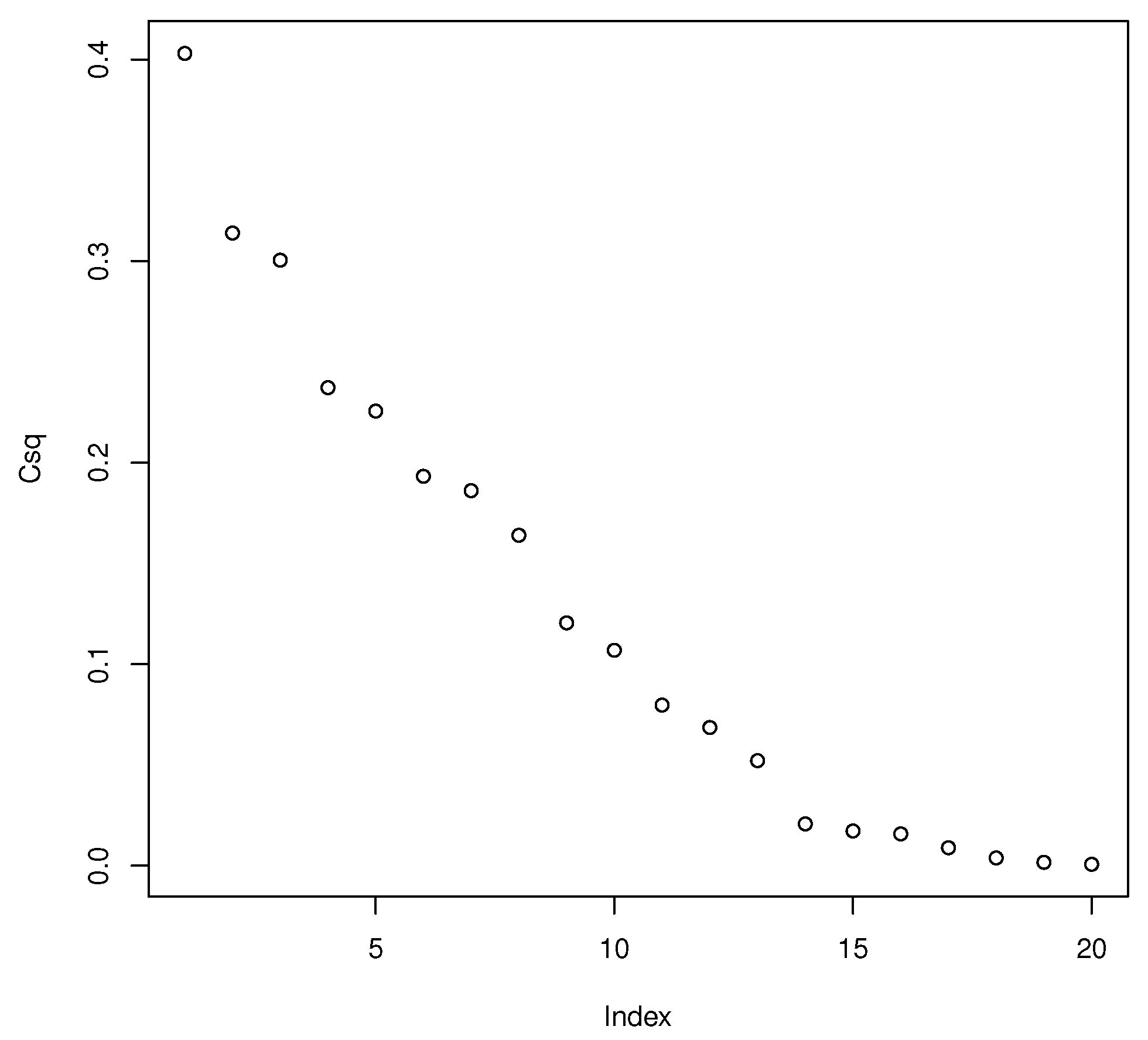
The [40] pottery data have $n=36$ pottery shards of Roman earthware produced between second century B.C. and fourth century A.D. Often the pottery was stamped by the manufacturer. A chemical analysis was done for $p=20$ chemicals (variables), the types of pottery were 1, Arretine; 2, not Arretine; 3, North Italian; 4, Central Italian; and 5, questionable origin. These codes were used for the response variable Y. Figure 1 shows the SC scree plot for this data set. Seven of the predictors ($x_7,x_{16},x_9,x_{20},x_{12},x_2,x_{11}$), had little correlation with Y. Changing the codes of the last 4 groups to 0 (binary response) gave a similar plot (not shown). Some output is shown below.

zy <-pottery[,1]

zx <- pottery[,-1]

SCscree(zx,zy)

$csums

  [1] 0.1599179 0.2844740 0.4036888 0.4978070 0.5873033 0.6639728 0.7378077

  [8] 0.8028591 0.8506671 0.8930894 0.9247144 0.9519310 0.9726192 0.9808558

[15] 0.9876990 0.9939687 0.9975125 0.9990487 0.9997179 1.0000000

$indx

  [1]  5  4 17  1 10  8  6 13 18 14 15 19  3  7 16  9 20 12  2 11

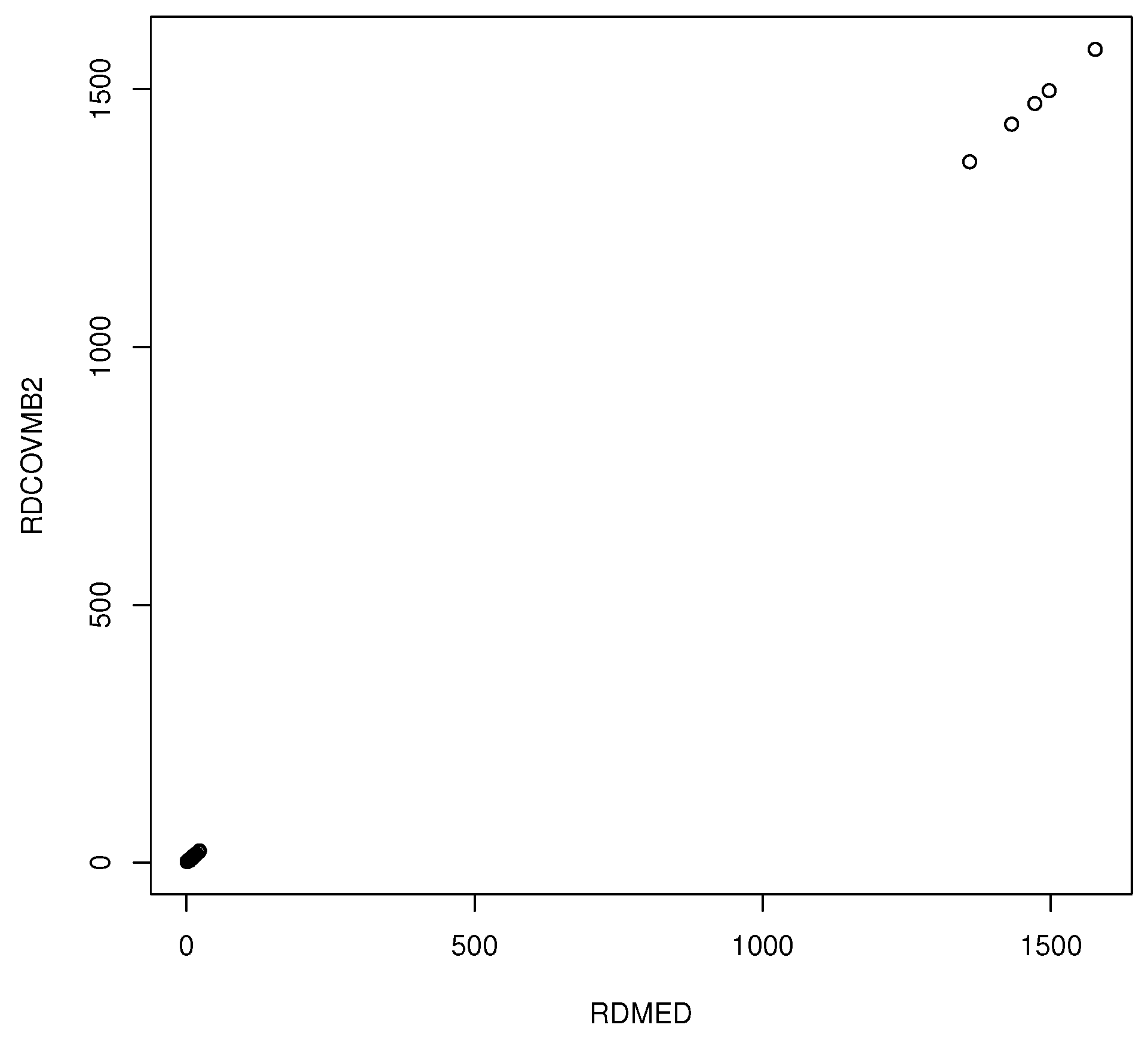
The function ddplot5 plots the Euclidean distances from the coordinatewise median versus the Euclidean distances from the covmb2 location estimator. Typically, the plotted points in this DD plot cluster about the identity line, and outliers appear in the upper-right corner of the plot with a gap between the bulk of the data and the outliers.

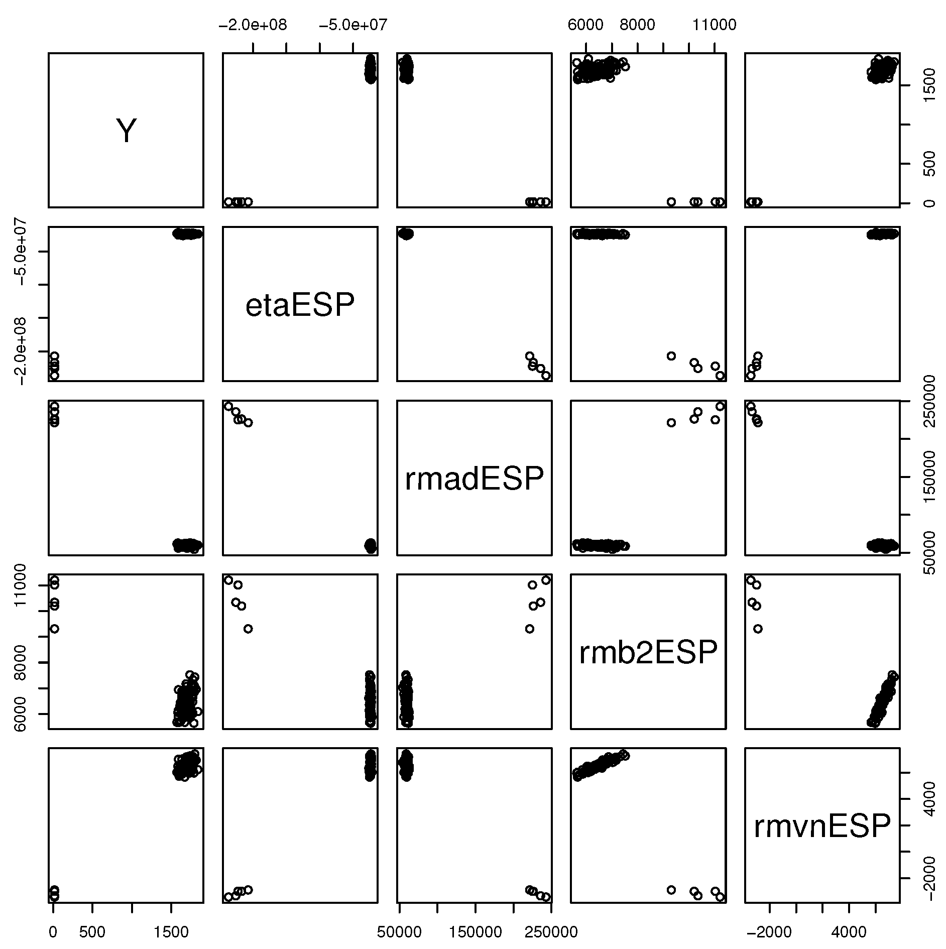
The function rcovxy yields the classical and three robust estimators of $\mathsf{\eta }={\mathbf{\Sigma }}_{\mathit{x}Y}$, and it makes a scatterplot matrix of the four estimated sufficient predictors ${\widehat{\mathsf{\eta }}}^T\mathit{x}$ and Y. Only two robust estimators are made if $n\le 2.5p$.

Example 3.

For the [41] data with multiple linear regression, height was the response variable while an intercept, head length, nasal height, bigonal breadth, and cephalic index were used as predictors in the multiple linear regression model. Observation 9 was deleted since it had missing values. Five individuals, cases 61–65, were reported to be about 0.75 inches tall with head lengths well over five feet!

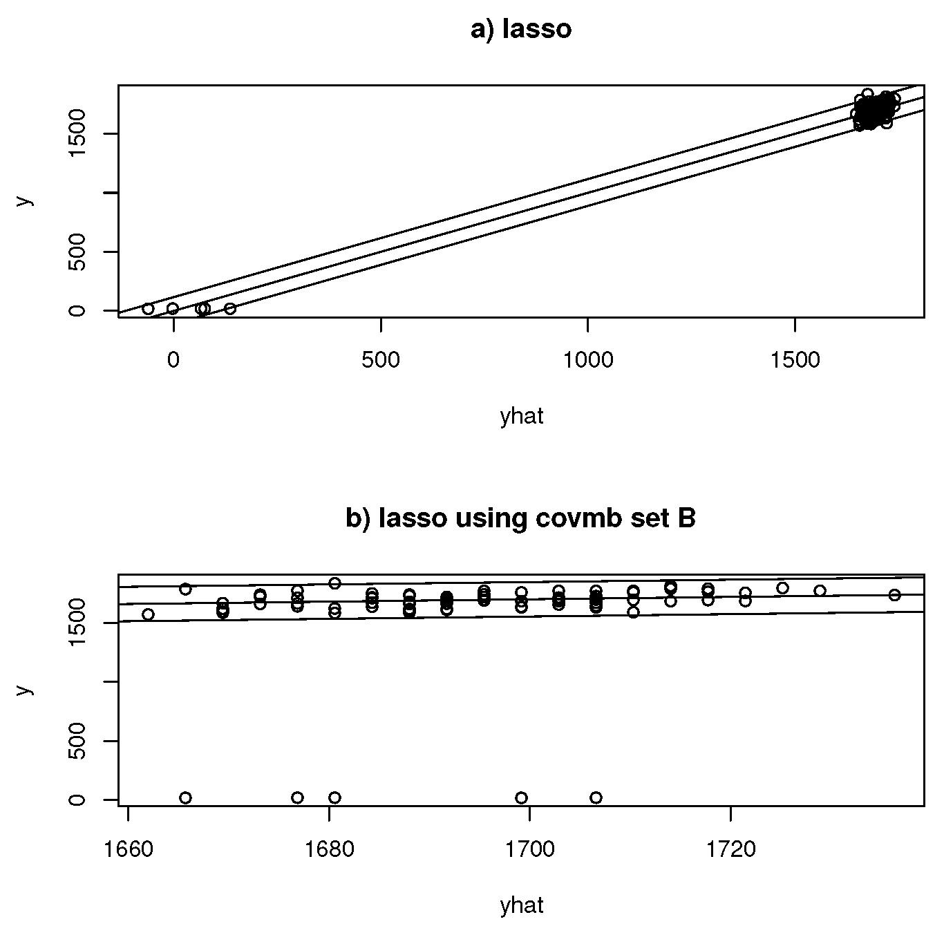
Figure 2a shows the response plot for lasso. The identity line passes right through the outliers which are obvious because of the large gap. Figure 2b shows the response plot from lasso for the cases in the covmb2 set B applied to the predictors, and the set B included all of the clean cases and omitted the 5 outliers. The response plot was made for all of the data, including the outliers. Prediction interval bands are also included for both plots. Both plots are useful for outlier detection, but the method for plot Figure 2b is better for data analysis as follows: impossible outliers should be deleted or given 0 weight, we do not want to predict that some people are about 0.75 inches tall, and we do want to predict that the people were about 1.6 to 1.8 m tall. Figure 3 shows the DD plot made using ddplot5. The five outliers are in the upper-right corner. Figure 4 shows the plot made using rcovxy. The five outliers are easy to detect, and the covmb2 estimator of ${\widehat{\mathbf{\Sigma }}}_{\mathit{x}Y}^T\mathit{x}$, denoted by rmb2ESP, linearized the data in the upper row.

4. Discussion

Detecting outliers, eliminating weak predictors, and recognizing that ${\widehat{\mathsf{\beta }}}_I$ estimates ${\mathsf{\beta }}_I$ are important techniques for high-dimensional statistics. Another useful technique is to fit several high-dimensional estimators and choose the one that minimizes some criterion, such as 5-fold cross validation. For multiple linear regression, useful estimators include lasso, model selection PLS, ridge regression, et cetera, using all of the predictors and deleting weak predictors. Using several estimators for high-dimensional data increases the chance of getting a good fit to the data.

Lasso often works well on high-dimensional data sets if there are strong predictors. Lasso also deletes weak predictors, and ${\widehat{\mathsf{\beta }}}_I$ often estimates ${\mathsf{\beta }}_I$. PLS often works well on high-dimensional chemometrics data sets, but it is not real clear why PLS works well when ${\widehat{\mathit{\gamma }}}_j$ is not a good estimator of ${\mathit{\gamma }}_j$. The PLS literature often assumes that $Y|\mathit{x}=$$Y|{\mathsf{\beta }}_{kPLS}^T\mathit{x}$ where ${\mathsf{\beta }}_{kPLS}$ is the population parameter for the k-component PLS estimator. Ref.  [12] showed that this PLS assumption tends to be quite strong.

The R software was used. See [42]. Programs are available from the collection of R functions slpack.txt, available from (http://parker.ad.siu.edu/Olive/slpack.txt, accessed on 30 June 2025). Proofs for Equation (4) and Theorems 1 and 2 were not given, but they are available from preprints of the corresponding published papers from (http://parker.ad.siu.edu/Olive/preprints.htm, accessed on 30 June 2025).

The covmb2 estimator attempts to give a robust dispersion estimator that reduces the bias by using a big ball about ${\mathrm{MED}}_j$ instead of a ball that contains half of the cases. The median ball is the hypersphere centered at the coordinatewise median with radius $r=\mathrm{MED}(D_i(\mathrm{MED}\left(\mathit{W}\right),{\mathit{I}}_p),i=1,\dots ,n)$ that tends to contain $(n+1)/2$ of the cases if n is odd. The slpack function getB gives the set B of cases that got weight 1 along with the index indx of the case numbers that got weight 1.

The function corrlar produces the regularized correlation matrices Rd $=\mathit{R}(\delta ,0)$ and Rt $=\mathit{R}(\delta ,\tau )$ given a correlation matrix, condition number c, and threshold tau with $\tau =0.05$ the default. The function SCscree makes the SC scree plot.

References

1. Cook, R.D.; Forzani, L. Partial Least Squares Regression: And Related Dimension Reduction Methods; Chapman and Hall/CRC: Boca Raton, FL, USA, 2024. [Google Scholar]
2. Hastie, T.; Tibshirani, R.; Friedman, J. The Elements of Statistical Learning: Data Mining, Inference, and Prediction, 2nd ed.; Springer: New York, NY, USA, 2009. [Google Scholar]
3. James, G.; Witten, D.; Hastie, T.; Tibshirani, R. An Introduction to Statistical Learning with Applications in R, 2nd ed.; Springer: New York, NY, USA, 2021. [Google Scholar]
4. Chun, H.; Keleş, S. Sparse partial least squares regression for simultaneous dimension reduction and predictor selection. J. R. Stat. Soc. Ser. B 2010, 72, 3–25. [Google Scholar] [CrossRef] [PubMed]
5. Olive, D.J.; Hawkins, D.M. Variable selection for 1D regression models. Technometrics 2005, 47, 43–50. [Google Scholar] [CrossRef]
6. Mallows, C. Some comments on Cp. Technometrics 1973, 15, 661–676. [Google Scholar]
7. Rathnayake, R.C.; Olive, D.J. Bootstrapping some GLMs and survival regression models after variable selection. Commun. Stat. Theory Methods 2023, 52, 2625–2645. [Google Scholar] [CrossRef]
8. Gelman, A.; Carlin, J. Some natural solutions to the p-value communication problem-and why they won’t work. J. Am. Stat. Assoc. 2017, 112, 899–901. [Google Scholar] [CrossRef]
9. Nester, M.R. An applied statistician’s creed. J. R. Stat. Soc. Ser. C 1996, 45, 401–410. [Google Scholar] [CrossRef]
10. Tukey, J.W. The philosophy of multiple comparisons. Stat. Sci. 1991, 6, 100–116. [Google Scholar] [CrossRef]
11. Cox, D.R. Regression models and life-tables. J. R. Stat. Soc. Ser. B 1972, 34, 187–220. [Google Scholar] [CrossRef]
12. Olive, D.J.; Zhang, L. One component partial least squares, high dimensional regression, data splitting, and the multitude of models. Commun. Stat. Theory Methods 2025, 54, 130–145. [Google Scholar] [CrossRef]
13. Artigue, H.; Smith, G. The principal problem with principal components regression. Cogent Math. Stat. 2019, 6, 1622190. [Google Scholar] [CrossRef]
14. Cook, R.D. Fisher lecture: Dimension reduction in regression. Stat. Sci. 2007, 22, 1–26. [Google Scholar] [CrossRef]
15. Cook, R.D. Principal components, sufficient dimension reduction, and envelopes. Ann. Rev. Stat. Appl. 2018, 5, 533–559. [Google Scholar] [CrossRef]
16. Zhang, J.; Chen, X. Principal envelope model. J. Stat. Plan. Infer. 2020, 206, 249–262. [Google Scholar] [CrossRef]
17. Brown, P.J. Measurement, Regression, and Calibration; Oxford University Press: New York, NY, USA, 1993. [Google Scholar]
18. Cook, R.D.; Forzani, L. PLS regression algorithms in the presence of nonlinearity. Chemom. Intell. Lab. Syst. 2021, 213, 104307. [Google Scholar] [CrossRef]
19. Mardia, K.V.; Kent, J.T.; Bibby, J.M. Multivariate Analysis; Academic Press: London, UK, 1979. [Google Scholar]
20. Cook, R.D.; Weisberg, S. Applied Regression Including Computing and Graphics; Wiley: New York, NY, USA, 1999. [Google Scholar]
21. Jung, S.; Marron, J.S. PCA consistency in high dimension low sample size context. Ann. Stat. 2012, 37, 4104–4130. [Google Scholar] [CrossRef]
22. Fan, J.; Lv, J. Sure independence screening for ultrahigh dimensional feature space. J. R. Stat. Soc. Ser. B 2008, 70, 849–911. [Google Scholar] [CrossRef]
23. Fan, J.; Song, R. Sure independence screening in generalized linear models with np-dimensionality. Ann. Stat. 2010, 38, 3217–3841. [Google Scholar] [CrossRef]
24. Mehmood, T.; Sæbø, S.; Liland, K.H. Comparison of variable selection methods in partial least squares regression. J. Chemom. 2020, 34, e3226. [Google Scholar] [CrossRef]
25. Tibshirani, R. Regression shrinkage and selection via the lasso. J. R. Stat. Soc. Ser. B 1996, 58, 267–288. [Google Scholar] [CrossRef]
26. Zou, H.; Hastie, T. Regularization and variable selection via the elastic net. J. R. Stat. Soc. Ser. B 2005, 67, 301–320. [Google Scholar] [CrossRef]
27. Basa, J.; Cook, R.D.; Forzani, L.; Marcos, M. Asymptotic distribution of one-component partial least squares regression estimators in high dimensions. Can. J. Stat. 2024, 52, 118–130. [Google Scholar] [CrossRef]
28. Cook, R.D.; Helland, I.S.; Su, Z. Envelopes and partial least squares regression. J. R. Stat. Soc. Ser. B 2013, 75, 851–877. [Google Scholar] [CrossRef]
29. Olive, D.J.; Alshammari, A.A.; Pathiranage, K.G.; Hettige, L.A.W. Testing with the one component partial least squares and the marginal maximum likelihood estimators. Commun. Stat. Theory Methods 2025. [Google Scholar] [CrossRef]
30. Su, Z.; Cook, R.D. Inner envelopes: Efficient estimation in multivariate linear regression. Biometrika 2012, 99, 687–702. [Google Scholar] [CrossRef]
31. Yuan, K.H.; Chan, W. Biases and standard errors of standardized regression coefficients. Psychometrika 2011, 76, 670–690. [Google Scholar] [CrossRef] [PubMed]
32. Neudecker, H.; Wesselman, A.M. The asymptotic variance matrix of the sample correlation matrix. Lin. Alg. Appl. 1990, 127, 589–599. [Google Scholar] [CrossRef]
33. Ledoit, O.; Wolf, M. A well-conditioned estimator for large-dimensional covariance matrices. J. Mult. Analys. 2004, 88, 365–411. [Google Scholar] [CrossRef]
34. Warton, D.I. Penalized normal likelihood and ridge regularization of correlation and covariance matrices. J. Am. Stat. Assoc. 2008, 103, 340–349. [Google Scholar] [CrossRef]
35. Datta, B.N. Numerical Linear Algebra and Applications; Brooks/Cole: Pacific Grove, CA, USA, 1995. [Google Scholar]
36. Rajapaksha, K.W.G.D.H.; Olive, D.J. Wald type tests with the wrong dispersion matrix. Commun. Stat. Theory Methods 2024, 53, 2236–2251. [Google Scholar] [CrossRef]
37. Hu, J.; Bai, Z. A review of 20 years of naive tests of significance for high-dimensional mean vectors and covariance matrices. Sci. China Math. 2016, 59, 2281–2300. [Google Scholar] [CrossRef]
38. Olive, D.J. Robust Multivariate Analysis; Springer: New York, NY, USA, 2017. [Google Scholar]
39. Hebbler, B. Statistics of Prussia. J. Stat. Soc. Lond. 1847, 10, 154–186. [Google Scholar] [CrossRef]
40. Wisseman, S.U.; Hopke, P.K.; Schindler-Kaudelka, E. Multielemental and multivariate analysis of Italian terra sigillata in the world heritage museum, university of Illinois at Urbana-Champaign. Archeomaterials 1987, 1, 101–107. [Google Scholar]
41. Buxton, L.H.D. The anthropology of Cyprus. J. R. Anthrop. Inst. Great Br. Irel. 1920, 50, 183–235. [Google Scholar] [CrossRef]
42. R Core Team. R: A Language and Environment for Statistical Computing; R Foundation for Statistical Computing: Vienna, Austria, 2024. [Google Scholar]
Figure 1. SC scree plot for pottery data.
Stats 08 00060 g001
Figure 2. Response plot for lasso and lasso applied to the covmb2 set B.
Stats 08 00060 g002
Figure 3. DD plot.
Stats 08 00060 g003
Figure 4. Diagnostics for OPLS and Σ ^ x Y .
Stats 08 00060 g004
Disclaimer/Publisher’s Note: The statements, opinions and data contained in all publications are solely those of the individual author(s) and contributor(s) and not of MDPI and/or the editor(s). MDPI and/or the editor(s) disclaim responsibility for any injury to people or property resulting from any ideas, methods, instructions or products referred to in the content.