On the Decision-Theoretic Foundations and the Asymptotic Bayes Risk of the Region of Practical Equivalence for Testing Interval Hypotheses

Abstract

Testing interval hypotheses is of huge relevance in the biomedical and cognitive sciences; for example, in clinical trials. Frequentist approaches include the proposal of equivalence tests, which have been used to study if there is a predetermined meaningful treatment effect. In the Bayesian paradigm, two popular approaches exist: The first is the region of practical equivalence (ROPE), which has become increasingly popular in the cognitive sciences. The second is the Bayes factor for interval null hypotheses, which was proposed by Morey et al. One advantage of the ROPE procedure is that, in contrast to the Bayes factor, it is quite robust to the prior specification. However, while the ROPE is conceptually appealing, it lacks a clear decision-theoretic foundation like the Bayes factor. In this paper, a decision-theoretic justification for the ROPE procedure is derived for the first time, which shows that the Bayes risk of a decision rule based on the highest-posterior density interval (HPD) and the ROPE is asymptotically minimized for increasing sample size. To show this, a specific loss function is introduced. This result provides an important decision-theoretic justification for testing the interval hypothesis in the Bayesian approach based on the ROPE and HPD, in particular, when sample size is large.

1. Introduction

Hypothesis testing is a central method in scientific research [1]. Traditional null hypothesis testing (henceforth called precise hypothesis testing) is considered with a precise null hypothesis $H_0$ and its set complement $H_1$ in the parameter space $\mathrm{\Theta }$, which, in the Bayesian approach, is typically a Borel space $(\mathrm{\Theta },\tau )$ with $\sigma$-algebra $\tau$, and in the frequentist approach, it is simply a set [2]:

$$\begin{array}{c}\hfill H_0:\theta ={\theta }_0{H}_1:\theta \ne {\theta }_0\end{array}$$

(1)

where ${\theta }_0\in \mathrm{\Theta }$. However, various authors have criticized that precise null hypothesis testing is inadequate in a variety of research situations, questioning the usefulness of this approach. One of the main critiques of precise hypothesis testing based on equality constraints is that such constraints are often not plausible for the context of research. Small violations of these equality constraints nearly always exist [3,4]. Concerning the questionable scientific standard of precise hypothesis testing in fields like medicine or cognitive science, Berger, Boukai, and Wang [5] noted the following:

“The decision whether or not to formulate an inference problem as one of testing a precise null hypothesis centers on assessing the plausibility of such an hypothesis. Sometimes this is easy, as in testing for the presence of extrasensory perception, or testing that a proposed law of physics holds. Often it is less clear. In medical testing scenarios, for instance, it is often argued that any treatment will have some effect, even if only a very small effect, and so exact equality of effects (between, say, a treatment and a placebo) will never occur.” Berger et al. [6] (p. 145)

Examples where the appropriateness of precise hypotheses may be questioned include exploratory research, measurements that include a non-negligible amount of error, and general complex phenomena in which simple statistical models at best can be interpreted as approximations to reality [5,7,8]. As exact equality of effects is unplausible in a variety of research contexts, interval hypotheses present an appealing alternative to precise hypotheses, at least in a variety of research settings in the medical, cognitive, and social sciences [7]. In contrast to precise null hypotheses, an interval hypothesis and its alternative are formalized as follows:

$$\begin{array}{c}\hfill H_0:\theta \in [{\theta }_0-c,{\theta }_0+c]H_1:\theta \notin [{\theta }_0-c,{\theta }_0+c]\end{array}$$

(2)

for some $c\in \mathrm{\Theta }$, where often $\mathrm{\Theta }:={\mathbb{R}}^n$. In the above, $\theta \in \mathrm{\Theta }$ is the parameter of interest and ${\theta }_0\in \mathrm{\Theta }$ is the null value of the precise null hypothesis $H_0:\theta ={\theta }_0$. In contrast to precise hypotheses, an interval hypothesis consists of an interval of parameter values, where $c\in \mathrm{\Theta }$ is determined from the available research context, domain-specific knowledge, or the available measurement precision, which is always finite. As a sidenote, in the vast majority of clinical phase II trials that aim to demonstrate the efficacy of a novel drug or treatment, a one-sided test for the binary variable success is of interest (where a success can have different interpretations, e.g., reduction of tumor volume [9,10]), see Zhou et al. [11] and Kelter and Schnurr [12]. While such a hypothesis often is formulated as

$$\begin{array}{c}\hfill H_0:\theta \le {\theta }_0\mathrm{versus}{H}_1:\theta >{\theta }_0\end{array}$$

for an efficacy threshold ${\theta }_0\in (0,1)$, in the majority of cases, values of ${\theta }_0$ close to 1 are deemed unrealistic a priori. Note that such cases also represent an interval hypothesis, which can be modeled with the region of practical equivalence (see next section).

The core idea behind an interval hypothesis is, therefore, that equality constraints can be tested only up to a limited precision.

Research Problem and Outline

In the Bayesian paradigm, two popular approaches exist: The first is the region of practical equivalence (ROPE), which has become increasingly popular in the cognitive sciences. The second is the Bayes factor for interval null hypotheses, which was proposed by Morey et al. [13]. However, while the ROPE is conceptually appealing, it lacks a clear decision-theoretic foundation like the Bayes factor. In this paper, a decision-theoretic justification for the ROPE procedure is derived for the first time, which shows that the Bayes risk of a decision rule is asymptotically minimized for increasing sample size.

Therefore, details on Bayesian approaches to interval hypothesis testing, including the ROPE and interval Bayes factors, are provided in Section 2. Then, in Section 3, a specific loss function is introduced for the ROPE. Then, the main result is provided by using this loss function. The main result gives an important decision-theoretic justification for testing interval hypotheses in the Bayesian approach via the ROPE. Section 4 reports the results of a simulation study, which yields recommendations for application of the results in practical settings. Section 5 provides a discussion of the result and concludes this paper.

2. Bayesian Approaches to Interval Hypothesis Testing

In this section, the two most popular approaches to Bayesian interval hypothesis testing are discussed briefly. The first approach is the region of practical equivalence, and the second approach is the Bayes factor. We primarily provide details on the Bayes factor because the decision-theoretic foundation (and its associated loss function) is very different from the one we introduce for the ROPE. Also, we stress that detailed decision-theoretic considerations for interval Bayes factors are, to our best knowledge, missing in the literature.

2.1. The Region of Practical Equivalence

To facilitate the shift to an estimation-oriented perspective, which employs the idea that hypothesis testing makes only sense up to a specific precision, ref. [14] proposed the region of practical equivalence. The concept itself appears under different names in a variety of scientific areas, and examples include the “interval of clinical equivalence”, “range of equivalence”, “equivalence interval”, “indifference zone”, “smallest effect size of interest,” and “good-enough belt” [14] (p. 185), where these formulations come from a wide spectrum of scientific contexts, see [15,16,17,18,19,20]. The concept of such a region has attracted researchers from diverse areas. The uniting idea of these concepts is to establish a region of practical equivalence around the null value ${\theta }_0$ of the precise null hypothesis $H_0:\theta ={\theta }_0$, where the region of practical equivalence expresses “the range of parameter values that are equivalent to the null value for current practical purposes”. [14] (p. 185). With a caution not to slip back into dichotomic black-and-white thinking, the following decision rule was proposed by Kruschke [21]:

• Reject the null value ${\theta }_0$ specified by $H_0:\theta ={\theta }_0$, if the 95% highest-posterior density interval (HPD) falls entirely outside the ROPE.
• Accept the null value ${\theta }_0$ specified by $H_0:\theta ={\theta }_0$, if the 95% HPD falls entirely inside the ROPE.

In the first case, with more than 95% probability, the parameter value is not inside the ROPE and therefore not practically equivalent to the null value ${\theta }_0$. A rejection of the null value ${\theta }_0$ then seems legitimate. In the second case, the parameter value is located inside the ROPE with at least 95% posterior probability and therefore is practically equivalent to the null value ${\theta }_0$. It is then legitimate to accept the null value ${\theta }_0$. Of course, it would also be possible to accept the null value ${\theta }_0$ only when the entire posterior (or equivalently, the 100% HPD) is located inside the ROPE, which leads to an even stricter decision rule.

However, in his proposal, Kruschke [21] treats the ROPE as a decision rule to accept the null value, reject it, or make no decision at all (personal communication with the author). In his interpretation, the ROPE does not mimic a hypothesis test and is not interpreted as an interval hypothesis $H_0:\theta \in [{\theta }_0-c,{\theta }_0+c]$ for some boundary $c>0$. As a consequence, Kruschke [21] accepts the null value ${\theta }_0$ instead of the interval hypothesis $H_0:\theta \in [{\theta }_0-c,{\theta }_0+c]$ for some boundary $c>0$ whenever the 95% HPD is located inside the ROPE.

Although this perspective can be taken, other authors have argued for an interpretation of the ROPE as an interval hypothesis [12,22,23,24,25,26]. Reconsidering the decision rule of Kruschke [21] based on the ROPE and HPD, in the first case, more than 95% of the posterior probability mass is located outside the interval hypothesis $H_0:\theta \in [{\theta }_0-c,{\theta }_0+c]$, where $c>0$ is the ROPE boundary. That is, if the ROPE is specified as $R=[{\theta }_0-c,{\theta }_0+c]$ around the null value ${\theta }_0\in \mathrm{\Theta }$, one can interpret it as the interval hypothesis area used in the interval hypotheses $H_0:\theta \in [{\theta }_0-c,{\theta }_0+c]$ and $H_1:\theta \notin [{\theta }_0-c,{\theta }_0+c]$. A rejection of the interval hypothesis $H_0:\theta \in [{\theta }_0-c,{\theta }_0+c]$ in the first case then seems legitimate. In the second case, the parameter value is located inside the ROPE $R=[{\theta }_0-c,{\theta }_0+c]$ with at least 95% posterior probability, and therefore more than 95% of the posterior probability mass are located inside the interval hypothesis $H_0:\theta \in [{\theta }_0-c,{\theta }_0+c]$. It is then legitimate to accept the null hypothesis $H_0$. In this paper, the interpretation of the ROPE as an interval hypothesis is adopted. Notice, however, that the main result of this paper given in Theorem 1 holds from both perspectives, no matter if the ROPE is interpreted as an interval hypothesis or as an extra cushion around the sharp point null value ${\theta }_0$, where values inside this cushion are interpreted as practically equivalent to ${\theta }_0$.

2.2. Bayes Factors for Interval Hypotheses

A second category of Bayesian approaches for testing interval hypotheses is based on the Bayes factor. The Bayes factor $B{F}_{01}^{\pi }$ is a predictive updating factor that measures the change in relative beliefs about both hypotheses $H_0$ and $H_1$ under consideration given the data x:

$$\begin{array}{c}\hfill B{F}_{01}^{\pi }\left(x\right):={\displaystyle \frac{P^{\pi }(\theta \in {\mathrm{\Theta }}_0|x)}{P^{\pi }(\theta \in {\mathrm{\Theta }}_1|x)}}/{\displaystyle \frac{\pi (\theta \in {\mathrm{\Theta }}_0)}{\pi (\theta \in {\mathrm{\Theta }}_1)}}\end{array}$$

(3)

Here, the superscript $\pi$ indexes the prior distribution $\pi$ assigned to the parameter $\theta \in \mathrm{\Theta }$, and $P^{\pi }(·|x)$ denotes the posterior distribution based on the prior $\pi$ and observed data x. The Bayes factor $B{F}_{01}^{\pi }$ is the ratio of the two marginal likelihoods $p\left(x\right|H_0)$ and $p\left(x\right|H_1)$ of both models, and these are calculated by integrating out the respective model parameters according to their prior distributions. Generally, the calculation of the marginal likelihoods quickly becomes complex for non-trivial models [27,28], and in high-dimensional settings, numerical techniques are often preferred as a consequence [29].

Despite these computational issues, the Bayes factor has an appealing decision-theoretic justification. Let $\mathrm{\Theta }:={\mathrm{\Theta }}_0\cup {\mathrm{\Theta }}_1$ be a disjunct partition of the parameter space $\mathrm{\Theta }$ into the null hypothesis $H_0:\theta \in {\mathrm{\Theta }}_0$ and its alternative $H_1:\theta \in {\mathrm{\Theta }}_1$ with ${\mathrm{\Theta }}_0\cap {\mathrm{\Theta }}_1=\varnothing$. Here, $H_0$ can be a precise or interval hypothesis. The weighted 0–1 loss function is given as follows:

$$\begin{array}{c}\hfill L(\theta ,\phi ):=\left\{\begin{array}{c}0,\mathrm{if}\phi ={\mathbb{1}}_{{\mathrm{\Theta }}_0}\left(\theta \right)\hfill \\ a_0,\mathrm{if}\theta \in {\mathrm{\Theta }}_0\mathrm{and}\phi =0\hfill \\ a_1,\mathrm{if}\theta \notin {\mathrm{\Theta }}_0\mathrm{and}\phi =1\hfill \end{array}\right.\end{array}$$

(4)

Here, $\phi$ is a decision rule based on the observed data x, where $\phi =1$ means accept $H_0$ and $\phi =0$ means accept $H_1$. The quantities $a_0,a_1>0$ are the losses associated with a false-positive and false-negative decision. The associated Bayes estimator for a prior distribution $\pi$ for the parameter $\theta$ can be given as follows:

$$\begin{array}{c}\hfill {\phi }^{\pi }\left(x\right)=\left\{\begin{array}{c}1,\mathrm{if}{P}^{\pi }(\theta \in {\mathrm{\Theta }}_0|x)>{\displaystyle \frac{a_1}{a_0+a_1}}\hfill \\ 0,\mathrm{otherwise}\hfill \end{array}\right.\end{array}$$

(5)

For details, see Robert [30] (Proposition 5.2.2). In the above, $P^{\pi }$ is the posterior based on the prior $\pi$, and for the losses $a_0=a_1=1$, the Bayes estimator ${\phi }^{\pi }\left(x\right)$ can be formulated as follows: Accept $H_0$ when the posterior probability of $H_0$ is larger than $0.5$, that is, $P^{\pi }(\theta \in {\mathrm{\Theta }}_0|x)>0.5$; otherwise, accept $H_1$. The Bayes factor is completely equivalent to the posterior probability of the null hypothesis from a decision-theoretic point of view. Using the loss function (4), $H_0$ is accepted when

$$\begin{array}{c}\hfill B{F}_{01}^{\pi }\left(x\right)>{\displaystyle \frac{a_1}{a_0}}/{\displaystyle \frac{\pi (\theta \in {\mathrm{\Theta }}_0)}{\pi (\theta \in {\mathrm{\Theta }}_1)}}\end{array}$$

(6)

because

$$\begin{array}{cc}\hfill B{F}_{01}^{\pi }\left(x\right)>{\displaystyle \frac{a_1}{a_0}}/{\displaystyle \frac{\pi (\theta \in {\mathrm{\Theta }}_0)}{\pi (\theta \in {\mathrm{\Theta }}_1)}}& \iff {\displaystyle \frac{P^{\pi }(\theta \in {\mathrm{\Theta }}_0|x)}{P^{\pi }(\theta \in {\mathrm{\Theta }}_1|x)}}/{\displaystyle \frac{\pi (\theta \in {\mathrm{\Theta }}_0)}{\pi (\theta \in {\mathrm{\Theta }}_1)}}>{\displaystyle \frac{a_1}{a_0}}/{\displaystyle \frac{\pi (\theta \in {\mathrm{\Theta }}_0)}{\pi (\theta \in {\mathrm{\Theta }}_1)}}\hfill \end{array}$$

(7)

$$\begin{array}{cc}\hfill & \iff {\displaystyle \frac{P(\theta \in {\mathrm{\Theta }}_0|x)}{P(\theta \in {\mathrm{\Theta }}_1|x)}}>{\displaystyle \frac{a_1}{a_0}}\iff P(\theta \in {\mathrm{\Theta }}_0|x)>{\displaystyle \frac{a_1}{a_0}}P(\theta \in {\mathrm{\Theta }}_1|x)\hfill \end{array}$$

(8)

$$\begin{array}{cc}\hfill & \iff P(\theta \in {\mathrm{\Theta }}_0|x)>{\displaystyle \frac{a_1}{a_0}}(1-P(\theta \in {\mathrm{\Theta }}_0|x))\hfill \end{array}$$

(9)

$$\begin{array}{cc}\hfill & \iff {\displaystyle \frac{a_0}{a_0}}P(\theta \in {\mathrm{\Theta }}_0|x)+{\displaystyle \frac{a_1}{a_0}}P(\theta \in {\mathrm{\Theta }}_0|x)>{\displaystyle \frac{a_1}{a_0}}\hfill \end{array}$$

(10)

$$\begin{array}{cc}\hfill & \iff {\displaystyle \frac{a_0+a_1}{a_0}}P(\theta \in {\mathrm{\Theta }}_0|x)>{\displaystyle \frac{a_1}{a_0}}\hfill \end{array}$$

(11)

$$\begin{array}{cc}\hfill & \iff P^{\pi }(\theta \in {\mathrm{\Theta }}_0|x)>{\displaystyle \frac{a_1}{a_0+a_1}}\hfill \end{array}$$

(12)

where the last inequality is the Bayes estimator given in Equation (5). Consequently, when using the decision rule $B{F}_{01}^{\pi }\left(x\right)>{\displaystyle \frac{a_1}{a_0}}/{\displaystyle \frac{\pi (\theta \in {\mathrm{\Theta }}_0)}{\pi (\theta \in {\mathrm{\Theta }}_1)}}$, one uses the Bayes estimator in Equation (5), which justifies the Bayes factor from a decision-theoretic point of view. For identical losses $a_0=a_1$ for false-positive and false-negative decisions and identical prior weights $\pi (\theta \in {\mathrm{\Theta }}_0)=\pi (\theta \in {\mathrm{\Theta }}_1)=0.5$ of the null and alternative hypothesis $H_0$ and $H_1$, the null hypothesis $H_0$ is accepted if $B{F}_{01}^{\pi }\left(x\right)>1$, which looks more familiar.

As the Bayes factor enjoys the above outlined decision-theoretic justification, Morey and Rouder [13] derived Bayes factors for testing interval null hypotheses. They distinguish between three types of hypotheses: The nil hypothesis, which states that a parameter or effect is precisely zero, the null hypothesis, which may be restricted to a nil hypothesis but may also allow for values which deviate slightly from the nil, and the default hypothesis, which refers to a hypothesis which is assumed to be true unless sufficient evidence is presented against it. Morey and Rouder [13] take the default position that the nil hypothesis never holds to arbitrary precision; that is, there is always some kind of effect. As a consequence, they aim to establish a region of parameter values around the nil hypothesis which are not “materially significant”, referring to the early ideas of Hodges and Lehmann [31]. This region contains all parameter values which are considered too small to be meaningfully different from zero. Details on the different types and the derivations of the Bayes factors in the three models can be found in Morey and Rouder’s paper [13].

Although the Bayes factors given in Morey and Rouder’s paper [13] present a decision-theoretically justified procedure for interval hypothesis testing in the Bayesian paradigm, a disadvantage of the Bayes factor, as mentioned by Robert [32] and Tendeiro and Kiers [33], is its dependence on the prior used for the model parameters. We stress that often, Bayes factors are criticized due to their dependence on the prior distribution, see Robert [32] or Tendeiro and Kiers [33]. The ROPE is often seen as quite robust to the selected prior hyperparameters [24], but it is still influenced by the latter. An entirely different mode of inference would consist of using pure likelihood ratios, as championed by [34]. This approach would, however, require an analogue concept to the ROPE that is based solely on likelihood ratios. While interesting in itself, developing such an approach is clearly outside the scope of the current manuscript. A detailed discussion about the premises of Bayesian tests is also given in the discussion between Ly and Wagenmakers [35] and Kelter [36]. In contrast, the ROPE is based on the posterior distribution, which, because of the well-known Bernstein–von Mises theorem, is asymptotically normal [37,38]. Consequently, the ROPE is quite robust to the prior selection, as discussed in Kruschke [21] and demonstrated by Makowski et al. [23] and Kelter [24]. However, by now, the ROPE lacks a decision-theoretic justification, which will be presented now.

3. Decision-Theoretic Foundation of the ROPE

In this section, the main result is presented. Although the ROPE has appealing practical properties like its robustness to the prior selection and wide applicability, it lacks a decision-theoretic justification. In contrast, the Bayes factor can be motivated from a decision-theoretic perspective as a formal Bayes rule, as shown in the previous section. The main result of this paper is given in Theorem 1 and shows that the decision rule based on the ROPE and HPD asymptotically minimizes the Bayes risk and can thus be called an asymptotic Bayes rule.

The following notation is used: A decision rule $\delta$ maps the observed sample data $x\in \mathcal{X}$, where x is an element of a measure space $(\mathcal{X},\mathcal{A})$ with $\sigma$-algebra $\mathcal{A}$ onto an action space $(\mathsf{\Delta },{\mathcal{A}}_{\mathsf{\Delta }})$, which is a measure space with $\sigma$-algebra ${\mathcal{A}}_{\mathsf{\Delta }}$:

$$\begin{array}{c}\hfill \delta :(\mathcal{X},\mathcal{A})\to (\mathsf{\Delta },{\mathcal{A}}_{\mathsf{\Delta }})\end{array}$$

(13)

A loss function $L:\mathrm{\Theta }\times \mathsf{\Delta }\to {\overline{\mathbb{R}}}_{+}$ is then introduced, where ${\overline{\mathbb{R}}}_{+}:={\mathbb{R}}_{+}\cup \infty$, which takes a parameter $\theta \in \mathrm{\Theta }$ and a decision (or action) $a\in \mathsf{\Delta }$ and returns the incurred loss $L(\theta ,a)$ when deciding for $\delta \left(x\right)=a$ when $\theta$ is true. In the Bayesian interpretation, $(\mathrm{\Theta },\tau )$ is another measure space, the parameter space. The loss function $L(\theta ,\delta (x\left)\right)$ depends on the decision made, which itself depends on the decision rule $\delta (·)$, which itself depends on the observed data $x\in \mathcal{X}$. To account for the uncertainty in the decision rule $\delta$, the risk function $R:\mathrm{\Theta }\times \mathcal{D}\to [0,\infty )$ is introduced, where $\mathcal{D}$ is the set of all (randomized) decision functions $\delta$:

$$\begin{array}{c}\hfill R(\theta ,\delta ):={\int }_{\mathcal{X}}\left({\int }_{\mathsf{\Delta }}L(\theta ,y)\delta (x,dy)\right)d{P}_{\theta }\left(x\right)\end{array}$$

(14)

In the above, the inner integral ${\int }_{\mathsf{\Delta }}L(\theta ,y)\delta (x,dy)$ is the loss incurred when using the decision rule $\delta$ for all possible decisions $\mathsf{\Delta }$ for the fixed parameter value $\theta$ and fixed sample $x\in \mathcal{X}$. The outer integral over $\mathcal{X}$ with respect to the measure $P_{\theta }\left(x\right)$, which is $P(X=x|\mathrm{\Theta }=\theta )$, accounts for the variability when observing $x\in \mathcal{X}$. That is, $P_{\theta }\left(x\right)$ is a probability measure on the sample space $(\mathcal{X},\mathcal{A})$ of the (identifiable parameterized, compare [39]) statistical model $\mathcal{P}:=\{P_{\theta }:\theta \in \mathrm{\Theta }\}$, which is assumed to represent the true data generating process (which is a family of probability measures in most situations). The outer integral averages the incurred loss over the sample space $\mathcal{X}$ in the sense that it computes the incurred loss for all observable $x\in \mathcal{X}$.

A Bayesian will argue that he does not know which value $\theta$ has, so although Equation (14) accounts for the uncertainty in observing $x\in \mathcal{X}$, it remains unclear for which parameter value (14) should be computed. Phrased differently, Equation (14) accounts for the randomness of the observed data $x\in \mathcal{X}$ and the randomness of the action $a\in \mathsf{\Delta }$, but it does not account for the randomness of the parameter $\theta \in \mathrm{\Theta }$. Therefore, the Bayesian statistician selects a prior distribution $\mu \in M^1(\mathrm{\Theta },\tau )$, where $M^1(\mathrm{\Theta },\tau )$ is the set of all probability measures on the parameter space $(\mathrm{\Theta },\tau )$ and averages the risk over the prior distribution:

$$\begin{array}{c}\hfill r(\mu ,\delta ):={\int }_{\mathrm{\Theta }}R(\theta ,\delta )d\mu \left(\theta \right)\end{array}$$

(15)

which is called the Bayes risk of decision rule $\delta$ with respect to the prior $\mu$. Substituting (14) into (15), $r(\mu ,\delta )$ can also be written as as follows:

$$\begin{array}{c}\hfill r(\mu ,\delta ):={\mathit{\int }}_{\mathrm{\Theta }}\left[{\int }_{\mathcal{X}}\left({\int }_{\mathsf{\Delta }}L(\theta ,y)\delta (x,dy)\right)d{P}_{\theta }\left(x\right)\right]d\mu \left(\theta \right)\end{array}$$

(16)

A decision rule $\delta$ is called a Bayes rule if it minimizes the Bayes risk, which is formalized as follows:

$$\begin{array}{c}\hfill r(\mu ,{\delta }_0)\le r(\mu ,\delta )\forall \delta \in \mathcal{D}\end{array}$$

(17)

A decision rule $\delta$ is called an asymptotic Bayes rule if it minimizes the Bayes risk asymptotically, which is formalized as follows:

$$\begin{array}{c}\hfill r(\mu ,{\delta }_0)\le r(\mu ,\delta )\forall \delta \in \mathcal{D}\mathrm{for}n\to \infty \end{array}$$

(18)

where n denotes the sample size of the observed data $x\in \mathcal{X}$.

In the following, a decision rule $\delta$ and a loss function $L(\theta ,\delta (x\left)\right)$ are introduced, for which the asymptotic Bayes risk is zero; that is, $r(\mu ,\delta )\underset{n\to \infty }{\overset{P}{\to }}0$. This presents a decision-theoretic justification for the ROPE + HPD procedure for testing interval hypotheses.

The ROPE + HPD decision rule $\delta$ allows us only to accept or reject the null value ${\theta }_0$ or to make no decision. This implies that $\mathsf{\Delta }:=\{d_A,d_R,d_N\}$, where $d_A$ means accept ${\theta }_0$ for practical purposes, $d_R$ means reject ${\theta }_0$ for practical purposes, and $d_N$ means make no decision. Acceptance of the null value ${\theta }_0$ is interpreted as acceptance of the interval hypothesis $H_0:\theta \in [{\theta }_0-c,{\theta }_0+c]$ specified by the ROPE $R=[{\theta }_0-c,{\theta }_0+c]$, as noted above, and rejection of the null value ${\theta }_0$ as rejection of the interval hypothesis $H_0:\theta \in [{\theta }_0-c,{\theta }_0+c]$.

The decision rule based on the HPD and ROPE is now defined as follows:

Definition 1

(ROPE decision rule). Let $\delta :(\mathcal{X},\mathcal{A})\to (\mathsf{\Delta },{\mathcal{A}}_{\mathsf{\Delta }})$, with $\mathsf{\Delta }:=\{d_A,d_R,d_N\}$ and ${\mathcal{A}}_{\mathsf{\Delta }}:=\mathcal{P}\left(\mathsf{\Delta }\right)$. The ROPE decision rule $\delta \left(x\right)$ is given as

$$\begin{array}{c}\hfill \delta \left(x\right):=\left\{\begin{array}{c}{d}_A,[a,b]\cap R=[a,b]\widehat{=}\mathrm{HPD}\mathrm{entirely}\mathrm{inside}\mathrm{ROPE}\hfill \\ d_R,[a,b]\cap R=\varnothing \widehat{=}\mathrm{HPD}\mathrm{entirely}\mathrm{outside}\mathrm{ROPE}\hfill \\ d_N,[a,b]\cap R\ne [a,b]\wedge [a,b]\cap R\ne \varnothing \widehat{=}\mathrm{partial}\mathrm{overlap}\hfill \end{array}\right.\end{array}$$

(19)

where $R\in \mathrm{\Theta }$ is the ROPE (e.g., $R=[{\theta }_0-c,{\theta }_0+c]$ for some $c\in \mathrm{\Theta }$, where often, $\mathrm{\Theta }:={\mathbb{R}}^n$) and $a<b$, where a and b are the boundaries of the α% HPD based on the posterior density $p\left(\theta \right|x)$ based on the observed data $x\in \mathcal{X}$.

The loss function is then defined as follows:

Definition 2

(ROPE loss function). Let $L:\mathrm{\Theta }\times \mathsf{\Delta }\to {\overline{\mathbb{R}}}_{+}$ with $\mathsf{\Delta }=\{d_A,d_R,d_N\}$. The ROPE loss function is given as follows:

$$\begin{array}{c}\hfill L(\theta ,\delta \left(x\right)):=\left\{\begin{array}{c}\underset{\mathit{HPD}\mathit{width}}{\underbrace{(b-a)}}+\underset{\begin{array}{c}\mathit{cost}\mathit{of}\mathit{parameter}\\ \mathit{not}\mathit{in}\mathit{HPD}\end{array}}{\underbrace{c_P·{\mathbb{1}}_{\theta \notin [a,b]}}}+\underset{\begin{array}{c}\mathit{cost}\mathit{of}\mathit{accept}\\ \mathit{when}\mathit{HPD}\mathit{is}\mathit{not}\mathit{in}\mathit{R}\end{array}}{\underbrace{c_A·{\mathbb{1}}_{[a,b]\cap R=\varnothing }}},\mathrm{if}\delta \left(x\right)=d_A\hfill \\ \underset{\mathit{HPD}\mathit{width}}{\underbrace{(b-a)}}+\underset{\begin{array}{c}\mathit{cost}\mathit{of}\mathit{parameter}\\ \mathit{not}\mathit{in}\mathit{HPD}\end{array}}{\underbrace{c_P·{\mathbb{1}}_{\theta \notin [a,b]}}}+\underset{\begin{array}{c}\mathit{cost}\mathit{of}\mathit{reject}\\ \mathit{when}\mathit{HPD}\mathit{is}\mathit{in}\mathit{R}\end{array}}{\underbrace{c_R·{\mathbb{1}}_{[a,b]\cap R=[a,b]}}},\mathrm{if}\delta \left(x\right)=d_R\hfill \\ \underset{\mathit{HPD}\mathit{width}}{\underbrace{(b-a)}}+\underset{\begin{array}{c}\mathit{cost}\mathit{of}\mathit{parameter}\\ \mathit{not}\mathit{in}\mathit{HPD}\end{array}}{\underbrace{c_P·{\mathbb{1}}_{\theta \notin [a,b]}}}+\underset{\begin{array}{c}\mathit{cost}\mathit{of}\mathit{no}\\ \mathit{decision}\end{array}}{\underbrace{c_N·{\mathbb{1}}_{[a,b]\cap R\ne [a,b]\wedge [a,b]\cap R\ne \varnothing }}},\mathrm{if}\delta \left(x\right)=d_N\hfill \end{array}\right.\end{array}$$

(20)

where $c_P,c_A,c_R,c_N>0$ are penalties associated with the parameter not being located inside the HPD, accepting the null hypothesis $H_0$ when the HPD is not located entirely inside the ROPE R, rejecting the null hypothesis $H_0$ when the HPD is located entirely inside the ROPE R, and with making no decision.

In all cases, the HPD width $(b-a)$ and the cost $c_P$ of the parameter not being inside the HPD contribute to the loss. If $\delta \left(x\right)=d_R$, the null value ${\theta }_0$ is rejected, and the additionally incurred loss is $c_R·{\mathbb{1}}_{[a,b]\cap R=[a,b]}$; that is, the constant $c_R>0$ if the HPD $[a,b]$ is located entirely inside the ROPE R (then, $[a,b]\cap R=[a,b]$). This situation occurs if the HPD is in the ROPE, but the parameter is still excluded from the HPD. This situation occurs when the consistency of the posterior distribution causes the HPD to be already located inside the ROPE, but the parameter $\theta$ is still excluded from the HPD, possibly due to a not sufficiently large sample size.

If $\delta \left(x\right)=d_A$, one accepts the null value ${\theta }_0$. The additional costs are $c_A·{\mathbb{1}}_{[a,b]\cap R=\varnothing }$; that is, the constant $c_A>0$ if the HPD $[a,b]$ is located entirely outside the ROPE R (then, $[a,b]\cap R=\varnothing$). Such a case could occur when the posterior concentrates outside the ROPE R, but one still accepts the null value ${\theta }_0$ included in the ROPE (or the interval hypothesis described by the ROPE, see the first section).

If $\delta \left(x\right)=d_N$, no decision is made, and the additional costs are $c_N>0$ when the HPD partially overlaps with the ROPE and with the complement of the ROPE (then, $[a,b]\cap R\ne [a,b]\wedge [a,b]\cap R\ne \varnothing$).

Thus, the proposed loss function consists of three main components: A loss that occurs when accepting the null value ${\theta }_0$ (or the associated interval hypothesis) although the HPD is not in the ROPE R, a loss of rejecting it when the HPD is in R, and a loss for making no decision. All three components seem reasonable.

From a second perspective, the loss function increases the loss gradually: First, the HPD width is smaller for larger sample sizes and thus vanishes to zero due to the posteriors consistency [39]. The cost of the parameter not being inside the HPD indicates that a second step is needed. In this case, the HPD is off in some way, meaning that due to randomness in the data, the HPD has not sufficiently captured the characteristics of the true data generating processes. The last and third step is the one described in the previous paragraph.

The main result in this paper shows that the decision rule $\delta$ specified in Definition 1 minimizes the Bayes risk $r(\mu ,\delta )$ in Equation (15) asymptotically under the loss function $L(\theta ,\delta (x\left)\right)$ specified in Definition 2.

Theorem 1.

The decision rule $\delta :(\mathcal{X},\mathcal{A})\to (\mathsf{\Delta },{\mathcal{A}}_{\mathsf{\Delta }})$, as specified in Definition 1, minimizes the asymptotic Bayes risk with respect to any proper prior $\mu \in M^1(\mathrm{\Theta },\tau )$ under the loss function in Definition 2. That is, $r(\mu ,\delta )\underset{n\to \infty }{\overset{P}{\to }}0$ and consequently, for any other decision rule $\tilde{\delta }:(\mathcal{X},\mathcal{A})\to (\mathsf{\Delta },{\mathcal{A}}_{\mathsf{\Delta }})$, we have $r(\mu ,\delta )\le r(\mu ,\tilde{\delta })$ asymptotically in probability for $n\to \infty$.

Proof. 

See Appendix A. □

The above result has a drawback, however. The loss function of Definition 1 includes the width of the HPD interval as a constant loss in any case, whether the action $d_A$, $d_R$ or $d_N$ is made (accept, reject, or stay neutral about the hypothesis specified by the ROPE R). However, for small to moderate amounts of data, the width of the HPD interval can be substantial, depending on the statistical model and its parameter space $\mathrm{\Theta }$ of interest. Thus, a less debatable decision rule would consist solely of the following:

▸

the loss for the parameter not being inside the HPD $[a,b]$ due to randomness in the observed sample $x\in \mathcal{X}$,

▸

the loss associated with accepting a hypothesis when the HPD is not inside R, the loss of rejecting a hypothesis when the HPD is inside R, and the loss of making no decision at all, respectively.

The first point is an inherent problem that can occur in small to moderately sized samples $x\in \mathcal{X}$. The second point is the natural cost one would associate with making an obviously wrong decision when the (consistent) posterior distribution shows that the ROPE does not include the true parameter ${\theta }_0$, but one rejects or accepts the hypothesis circumscribed by the ROPE R. Note that these two losses are the second and third summands in the loss function of Definition 1.

We will now extend Theorem 1 and show that even when omitting the width $(b-a)$ of the $\alpha \%$-HPD interval from it, it still remains an asymptotic Bayes rule. The important consequence is that as the width $(b-a)$ vanishes only for unrealistically large sample sizes $n\in \mathbb{N}$, this renders the loss function of Definition 1 and Theorem 1 a much more practically relevant result. This is due to the fact that while the width $(b-a)$ vanishes for only extremely large $n\in \mathbb{N}$, the convergence speed in Equations (A5) and () is much faster. Therefore, even in situations where the HPD width might be substantial due to using only a moderate or small amount of data, the decision-theoretic justification of the ROPE, as stated in Theorem 1, holds.

Definition 3

(Simplified ROPE loss function). Let $L:\mathrm{\Theta }\times \mathsf{\Delta }\to {\overline{\mathbb{R}}}_{+}$ with $\mathsf{\Delta }=\{d_A,d_R,d_N\}$. The simplified ROPE loss function is given as follows:

$$\begin{array}{c}\hfill L(\theta ,\delta \left(x\right)):=\left\{\begin{array}{c}\underset{\begin{array}{c}\mathit{cost}\mathit{of}\mathit{parameter}\\ \mathit{not}\mathit{in}\mathit{HPD}\end{array}}{\underbrace{c_P·{\mathbb{1}}_{\theta \notin [a,b]}}}+\underset{\begin{array}{c}\mathit{cost}\mathit{of}\mathit{accept}\\ \mathit{when}\mathit{HPD}\mathit{is}\mathit{not}\mathit{in}\mathit{R}\end{array}}{\underbrace{c_A·{\mathbb{1}}_{[a,b]\cap R=\varnothing }}},\mathrm{if}\delta \left(x\right)=d_A\hfill \\ \underset{\begin{array}{c}\mathit{cost}\mathit{of}\mathit{parameter}\\ \mathit{not}\mathit{in}\mathit{HPD}\end{array}}{\underbrace{c_P·{\mathbb{1}}_{\theta \notin [a,b]}}}+\underset{\begin{array}{c}\mathit{cost}\mathit{of}\mathit{reject}\\ \mathit{when}\mathit{HPD}\mathit{is}\mathit{in}\mathit{R}\end{array}}{\underbrace{c_R·{\mathbb{1}}_{[a,b]\cap R=[a,b]}}},\mathrm{if}\delta \left(x\right)=d_R\hfill \\ \underset{\begin{array}{c}\mathit{cost}\mathit{of}\mathit{parameter}\\ \mathit{not}\mathit{in}\mathit{HPD}\end{array}}{\underbrace{c_P·{\mathbb{1}}_{\theta \notin [a,b]}}}+\underset{\begin{array}{c}\mathit{cost}\mathit{of}\mathit{no}\\ \mathit{decision}\end{array}}{\underbrace{c_N·{\mathbb{1}}_{[a,b]\cap R\ne [a,b]\wedge [a,b]\cap R\ne \varnothing }}},\mathrm{if}\delta \left(x\right)=d_N\hfill \end{array}\right.\end{array}$$

(21)

where $c_P,c_A,c_R,c_N>0$ are penalties associated with the parameter not being located inside the HPD, accepting the null hypothesis $H_0$ when the HPD is not located entirely inside the ROPE R, rejecting the null hypothesis $H_0$ when the HPD is located entirely inside the ROPE R, and with making no decision.

Now, given this simplified loss function, Theorem 1 still holds.

Theorem 2.

The decision rule $\delta :(\mathcal{X},\mathcal{A})\to (\mathsf{\Delta },{\mathcal{A}}_{\mathsf{\Delta }})$, as specified in Definition 1, minimizes the asymptotic Bayes risk with respect to any proper prior $\mu \in M^1(\mathrm{\Theta },\tau )$ under the loss function in Definition 3. That is, $r(\mu ,\delta )\underset{n\to \infty }{\overset{P}{\to }}0$, and consequently, for any other decision rule $\tilde{\delta }:(\mathcal{X},\mathcal{A})\to (\mathsf{\Delta },{\mathcal{A}}_{\mathsf{\Delta }})$, we have $r(\mu ,\delta )\le r(\mu ,\tilde{\delta })$ asymptotically in probability for $n\to \infty$.

Proof. 

See Appendix A. □

In closing this section, note that Theorems 1 and 2 do not contradict each other. Theorem 1 holds, but for the loss function in Definition 3, the inequality $r(\mu ,\delta )\le r(\mu ,\tilde{\delta })$ asymptotically in probability for $n\to \infty$, as ascertained in Theorem 1, becomes an equality. For a finite sample size $n\in \mathbb{N}$, the Bayes risk of the simplified ROPE loss function in Definition 3 is smaller then for the one given in Definition 2, particularly when the sample size $n\in \mathbb{N}$ of the observed data $x\in \mathcal{X}$ is small (and the HPD width in turn might be substantial).

4. Simulation Study

The result presented above provides a decision-theoretic justification of the ROPE for interval hypothesis testing, but it offers little guidance regarding how to make use of it in practical settings. While the result holds to any parametric statistical model and therefore is quite general, when the sample size is moderate, the key question is which of the costs $c_P,c_A,c_R,c_N$ dominates the total costs. In most realistic settings, it will be difficult if not even impossible to determine precise or even vague values for the costs $c_P,c_A,c_R,c_N$. Still, some comments can be made even without simulations: First, the costs $c_P·{\mathbb{1}}_{\theta \notin [a,b]}$ associated with the parameter not being located inside the HPD are independent of the decision made and indicate that the sample size is too small to capture the true parameter. The latter must happen eventually for large enough sample sizes due to the consistency of the posterior distribution [2]. As a consequence, the cost parameter $c_P$ will influence the total costs when the sample size is moderate or small. Second, it is well known from other research that the ROPE is slow, in the sense that it requires more samples than other Bayesian testing approaches to accept or reject a hypothesis [23,24,40]. As a consequence, for moderate sample sizes, the costs of no decision $c_N$ will dominate the total costs. In that case, the HPD partially overlaps with the ROPE, but is neither located entirely inside or outside of it.

An illustration of this phenomenon is given by simulating one of the most common testing problems, the two-sample t-test. We make use of the Bayesian t-test given by Rouder et al. [41] and four simulation scenarios: (1) $\delta =0$, so the null hypothesis $H_0:\delta \in [-0.2,0.2]$ holds. Here, we draw on the results of a large-scale meta-analysis of effect size magnitudes in medical research, comparing [42] to determine the ROPE boundaries $-0.2$ and $0.2$. (2) $\delta =-0.35$, which equals a small effect size according to Cohen [43], (3) $\delta =0.65$, which equals a medium effect size according to Cohen [43], and (4) $\delta =1.03$, which equals a large effect size according to Cohen [43]. Most relevant here are the results under no effect, a small effect, and a medium effect size, because these are much more realistic in applied research; compare [42]. We provide the percentage of the posterior probability inside the ROPE $R=[-0.2,0.2]$ for sample sizes $n=10,...,150$, which are common sample sizes per group in the cognitive and medical sciences. For each scenario, 10,000 datasets were simulated to compute the (1) mean posterior probability inside the ROPE and (2) the probability of the parameter being inside the HPD.

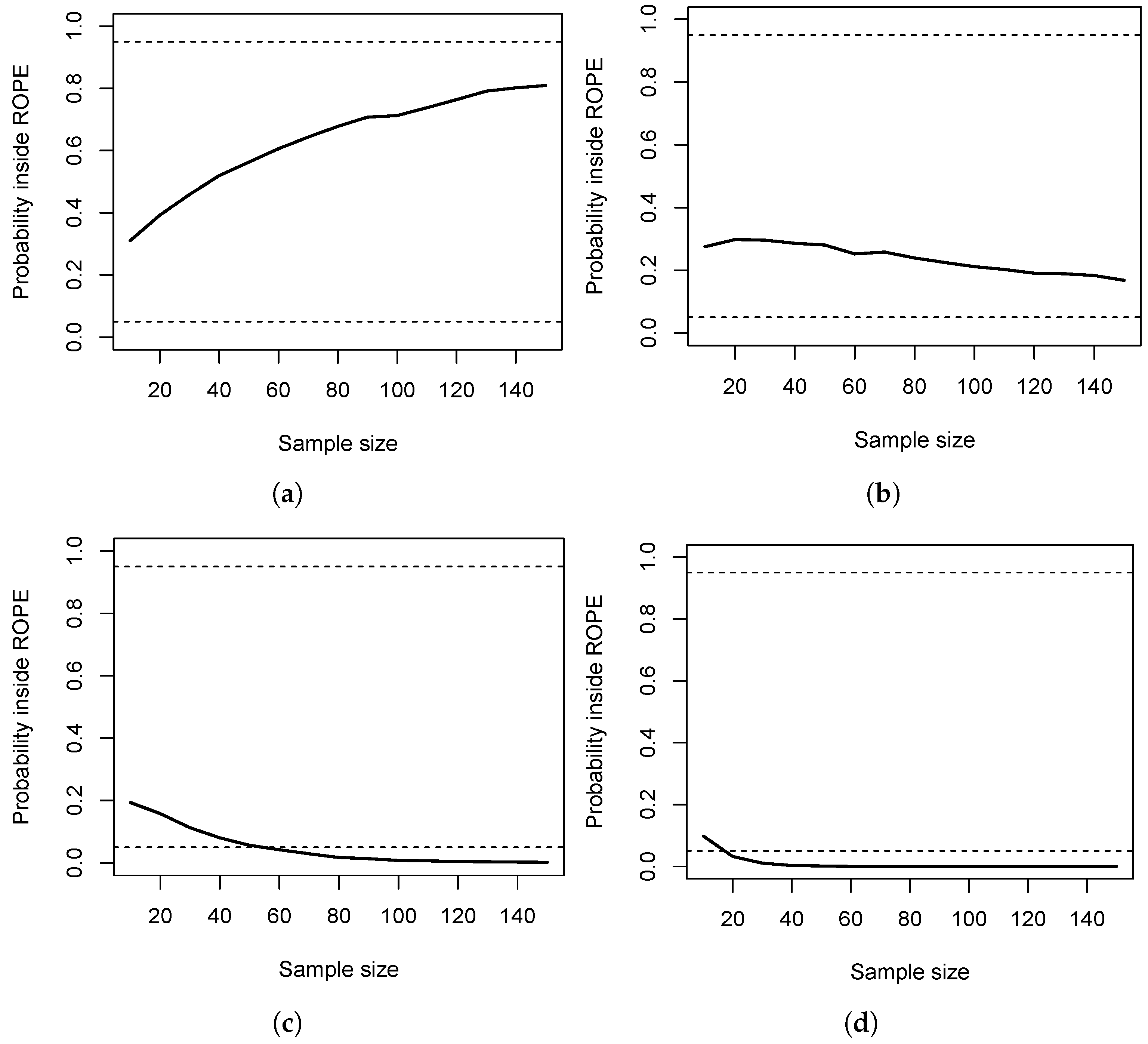
Figure 1 shows the results, and Figure 1a provides the results under $\delta =0$, so $H_0:\delta \in [-0,2,0.2]$ holds. The dashed horizontal lines show the values $95\%$ to accept $H_0$ and $5\%$ to reject it (in that case, 95% of the posterior probability is located inside $H_1:\delta \notin [-0.2,0.2]$, indicating to accept $H_1$). As can be seen, for all sample sizes, the situation remains indecisive, and there is a partial overlap between the ROPE and 95% HPD. As a consequence, the costs $c_N$ for making no decision fully dominate the entire costs in that scenario, that is, when $H_0$ holds. Figure 1b shows the results under a small effect size, and although $H_1$ is true now, the same situation holds. Even for $n=150$, the sample size is not large enough to reduce the posterior probability inside the ROPE $R=[-0.2,0.2]$ to below 5%. The costs $c_N$ entirely dominate the resulting costs. For a medium effect size, Figure 1c shows that for $n<60$, the costs of no decision $c_N$ again drive the entire costs. From $n\ge 60$ on, the correct decision is made, reducing the costs to zero. Figure 1d shows the situation for a large effect size, and here, even $\approx 20$ samples per group suffice to avoid any costs of making no decision $c_N$.

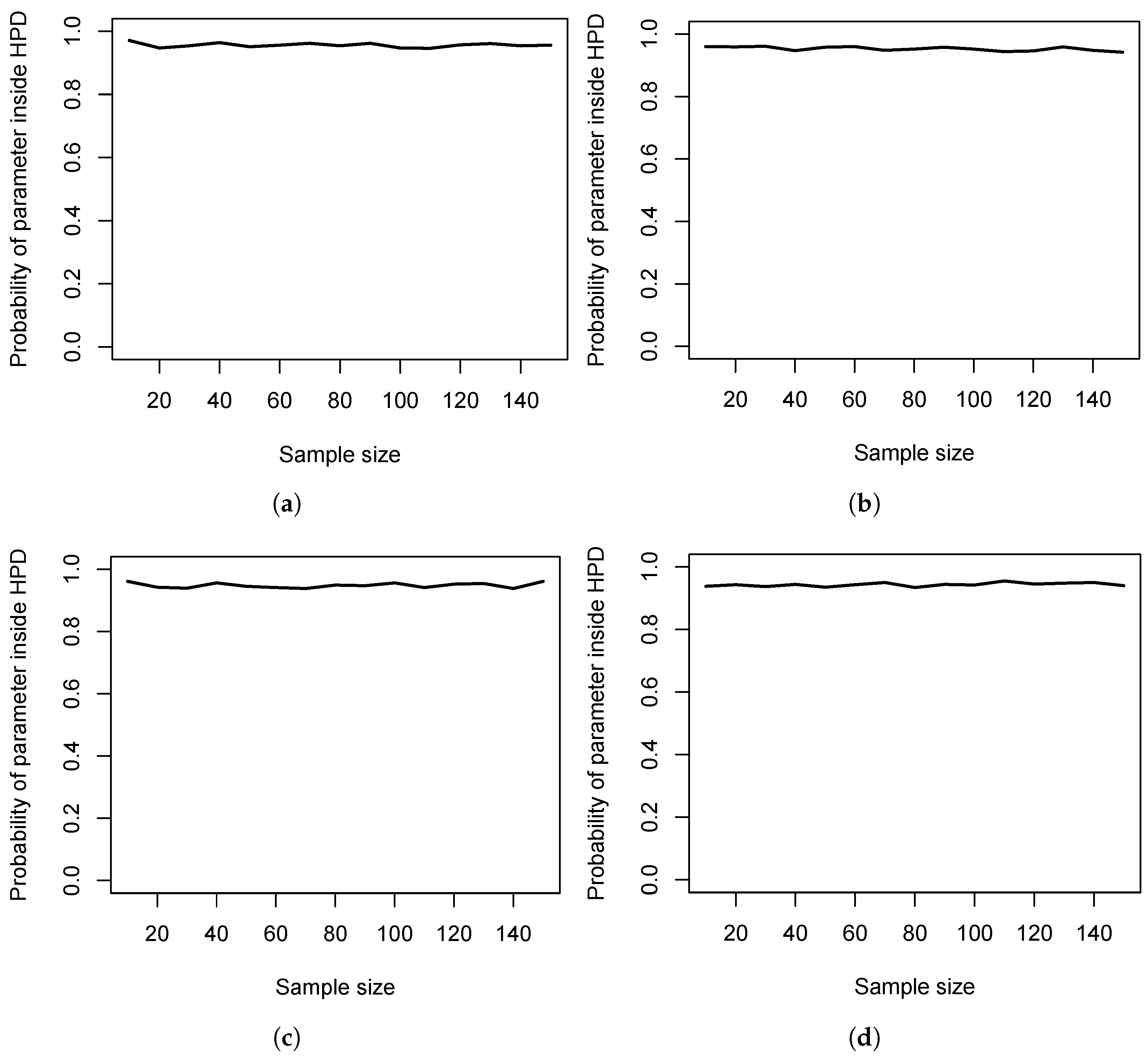
Figure 2 shows the probability of the HPD containing the true parameter $\delta$ for varying sample and effect sizes. Thus, the cost parameter $c_P$ is studied. In Figure 2a, the results under $H_0$ show that the true parameter $\delta =0$ is captured by the majority of HPDs independently of the sample size. This, most probably, is due to the Cauchy prior, which is used on $\delta$ in the model proposed by Rouder et al. [41] and which is centered around $\delta =0$. Figure 2b–d show that the same phenomenon holds for increasing effect size magnitude. Thus, the costs $c_P$ are much less relevant in realistically attainable sample sizes than the costs $c_N$ to stay indecisive.

We close this section with two comments. First, the values $c_P$ and $c_N$ clearly influence which costs are more relevant in a given situation. However, the probabilities in Figure 1 and Figure 2 show that the probability of staying indecisive is much larger than the probability of obtaining a HPD that does not cover the true parameter. Second, the costs $c_A$ and $c_R$ further influence the total costs. However, assigning explicit costs to acceptance or rejection of a hypothesis seems unrealistic for almost all applied research attempting to quantify the costs of a trial without a result equal to $c_N$. We therefore recommend studying the probability of obtaining an indecisive result for the statistical model at hand under the relevant scenarios, as shown in Figure 1. Additionally, we recommend selecting a sample size based on decision-theoretic grounds that yields a probability large enough to include the true parameter inside the HPD; compare Figure 2. Otherwise, the whole inference can be misleading.

5. Discussion

This section discusses the main result and its limitations. First and foremost, Theorem 1 provides a decision-theoretic justification of the ROPE procedure for testing interval hypotheses in the Bayesian paradigm. The latter has gained widespread attention from areas like statistical research [22], psychological research [21,23,44], and preclinical animal research [42]. Its simplicity and ease of application are appealing, but until now, the approach lacked a clear decision-theoretic justification. In this paper, such a justification is provided for the first time based on a decision rule that seems quite acceptable for most Bayesians.

The decision rule given in Definition 1 can be interpreted as a formalization of the ROPE method, as proposed by Kruschke [21]. The form of the selected loss function specified in Definition 2 needs to be justified further; for example, one could easily choose the trivial loss function $L(\theta ,\delta (x\left)\right)=(b-a)$, which is independent of the selected decision rule $\delta \left(x\right)$ and equals the width of the $\alpha$% HPD. This motivates Definition 3 and the important extension of Theorem 1 to this loss function; see Theorem 2.

The loss function $\delta$ given in Definition 3 incorporates four important desiderata: First, it contains an explicit penalty $c_A>0$ whenever the hypothesis $H_0$ is accepted, although the $\alpha$% HPD is not located entirely inside the ROPE R. Second, it contains an explicit penalty $c_R>0$ whenever the hypothesis $H_0$ is rejected, although the $\alpha$% HPD is located entirely inside the ROPE R. Third, it contains an explicit penalty $c_N>0$ whenever no decision is made, which is the case when the ROPE R and the $\alpha$% HPD partially overlap. Fourth, in all three cases (accept $H_0$, reject $H_0$, make no decision), a penalty $c_P>0$ is given if the $\alpha$% HPD does not include the true parameter $\theta \in \mathrm{\Theta }$. In such cases, the decision is based on a HPD that does not include the true parameter value, and the incurred loss naturally should be larger. Consequently, the loss function $L(\theta ,\delta (x\left)\right)$ given in Definition 3 is not trivial and justified from a practical point of view. Theorem 2 now guarantees that asymptotically, decisions made based on the decision rule in Definition 1 and the loss function in Definition 3 will minimize the Bayes risk.

An important limitation is that in small sample situations, little can be said about the incurred loss when following the decision rule $\delta$ under the loss function in Definition 2. Theorem 1 only guarantees that for large sample sizes n, the Bayes risk is minimized, but in a variety of research, only small to moderate samples can be acquired. Theorem 2 improves this situation drastically by using the simpler loss function in Definition 3, which excludes the HPD width $(b-a)$.

However, in small sample situations, the penalty terms $c_A,c_R$ and $c_N$ influence the resulting loss and risk even more substantially. Suppose, for example, the $\alpha$% HPD is located entirely outside the ROPE R for a small sample size $n\in \mathbb{N}$. Suppose further that the true parameter $\theta \in \mathrm{\Theta }$ is located inside the ROPE R, so the posterior will concentrate for increasing sample size n inside the ROPE R. In this case, the resulting loss for the small sample will be based on the case for which $\delta \left(x\right)=d_R$ in $L(\theta ,\delta (x\left)\right)$. Suppose now that the sample size is increased to $m>n$. Then, the ROPE and $\alpha$% HPD may overlap, and the resulting loss for the sample based on m observations will be based on the case for which $\delta \left(x\right)=d_N$ in $L(\theta ,\delta (x\left)\right)$. For growing sample size $m>>n$, eventually, the case is reached for which the resulting loss will be based on the case for which $\delta \left(x\right)=d_A$, but the speed of this process is not known. Consequently, when successively applying the decision rule (e.g., in the growing sample scenario outlined above), the total loss depends on the magnitudes of $c_A,c_R$ and $c_N$. For example, if the associated costs with making no decision $c_N$ are tiny, it matters little if a large sample size n is required until the posterior is located entirely inside the ROPE R. On the contrary, in situations where a decision is mandatory and cannot be deferred (the costs $c_N$ are large), the resulting loss may be substantial when the posterior is located inside the ROPE R only after observing a sample of very large size n. However, asymptotically, Theorem 2 guarantees that the Bayes risk will be minimized for any choice of $c_A,c_R$ and $c_N$, and a decision-theoretic justification of the popular decision rule based on the ROPE and HPD given in Definition 1 is provided.

Keeping this in mind, the result presented in this paper—as is the case with every asymptotic result, such as the laws of large numbers, the central limit theorem, or the Bernstein–von Mises-theorem—cannot provide a boundary $n_0\in \mathbb{N}$ so that for sample sizes $n>n_0$ one can be certain that the Bayes risk is minimized sufficiently. Still, it provides a decision-theoretic justification of statistical hypothesis testing based on the ROPE and HPD, which should not be understated in relevance. The reason is that the loss function in Definition 3 should be acceptable to most Bayesians, although the values of $c_A,c_R$ and $c_N$ will clearly differ from situation to situation.

Out simulation study results indicate that the costs $c_N$ could drive the total incurred loss when using the ROPE substantially. This is in line with previous research [23,24,40,45], and our results provide two important recommendations for applied research. First, when sample size is moderate, we highly recommend simulating the probability inside the ROPE for varying sample sizes and different scenarios under both $H_0$ and $H_1$, as in Figure 1. Then, the costs associated with no decision can be estimated for a given $c_N$. Second, the probability that the HPD contains the true parameter is crucial for reliable inference. We recommend simulating the latter as shown in Figure 2, also for varying sample sizes and relevant scenarios under $H_0$ and $H_1$ to select a minimum sample size that yields a large enough probability. This should safeguard against overconfidence and yield a Bayesian test for which Theorem 2 holds in an appealing way; that is, the total loss should be small.

Next to its robustness to the prior specification in large samples, this shows that the ROPE and HPD approach for testing interval hypotheses asymptotically minimize the Bayes risk for what seems like a natural loss function for a variety of situations. This result strengthens the justification of researchers applying interval hypothesis tests via the ROPE + HPD procedure in the Bayesian paradigm.

References

1. Wasserstein, R.L.; Schirm, A.L.; Lazar, N.A. Moving to a World Beyond “p<0.05”. Am. Stat. 2019, 73, 1–19. [Google Scholar] [CrossRef]
2. Schervish, M.J. Theory of Statistics; Springer: Berlin/Heidelberg, Germany, 1995. [Google Scholar]
3. Meehl, P.E. Theoretical risks and tabular asterisks: Sir Karl, Sir Ronald, and the slow progress of soft psychology. J. Consult. Clin. Psychol. 1978, 46, 806–834. [Google Scholar] [CrossRef]
4. Cohen, J. The earth is round (p < 0.05). Am. Psychol. 1994, 49, 997–1003. [Google Scholar] [CrossRef]
5. Berger, J.; Boukai, B.; Wang, Y. Unified Frequentist and Bayesian Testing of a Precise Hypothesis. Stat. Sci. 1997, 12, 133–160. [Google Scholar] [CrossRef]
6. Berger, J.; Brown, L.; Wolpert, R. A Unified Conditional Frequentist and Bayesian Test for fixed and sequential Hypothesis Testing. Ann. Stat. 1994, 22, 1787–1807. [Google Scholar] [CrossRef]
7. Ravenzwaaij, D.V.; Monden, R.; Tendeiro, J.N.; Ioannidis, J.P. Bayes factors for superiority, non-inferiority, and equivalence designs. BMC Med Res. Methodol. 2019, 19, 71. [Google Scholar] [CrossRef]
8. Berger, J.; Sellke, T. Testing a point null hypothesis: The irreconcilability of P values and evidence. J. Am. Stat. Assoc. 1987, 82, 112–122. [Google Scholar] [CrossRef]
9. Therasse, P.; Arbuck, S.G.; Eisenhauer, E.A.; Wanders, J.; Kaplan, R.S.; Rubinstein, L.; Verweij, J.; Glabbeke, M.V.; Oosterom, A.T.V.; Christian, M.C.; et al. New guidelines to evaluate the response to treatment in solid tumors. European Organization for Research and Treatment of Cancer, National Cancer Institute of the United States, National Cancer Institute of Canada. J. Natl. Cancer Inst. 2000, 92, 205–216. [Google Scholar] [CrossRef]
10. Eisenhauer, E.A.; Therasse, P.; Bogaerts, J.; Schwartz, L.H.; Sargent, D.; Ford, R.; Dancey, J.; Arbuck, S.; Gwyther, S.; Mooney, M.; et al. New response evaluation criteria in solid tumours: Revised RECIST guideline (version 1.1). Eur. J. Cancer 2009, 45, 228–247. [Google Scholar] [CrossRef]
11. Zhou, H.; Lee, J.J.; Yuan, Y. BOP2: Bayesian optimal design for phase II clinical trials with simple and complex endpoints. Stat. Med. 2017, 36, 3302–3314. [Google Scholar] [CrossRef]
12. Kelter, R.; Schnurr, A. The Bayesian Group-Sequential Predictive Evidence Value Design for Phase II Clinical Trials with Binary Endpoints. Stat. Biosci. 2024, 17, 442–478. [Google Scholar] [CrossRef]
13. Morey, R.D.; Rouder, J.N. Bayes Factor Approaches for Testing Interval Null Hypotheses. Psychol. Methods 2011, 16, 406–419. [Google Scholar] [CrossRef] [PubMed]
14. Kruschke, J.K.; Liddell, T. The Bayesian New Statistics: Hypothesis testing, estimation, meta-analysis, and power analysis from a Bayesian perspective. Psychon. Bull. Rev. 2018, 25, 178–206. [Google Scholar] [CrossRef] [PubMed]
15. Carlin, B.; Louis, T. Bayesian Methods for Data Analysis; Chapman & Hall, CRC Press: Boca Raton, FL, USA, 2009. [Google Scholar]
16. Freedman, L.S.; Lowe, D.; Macaskill, P. Stopping rules for clinical trials. Stat. Med. 1983, 2, 167–174. [Google Scholar] [CrossRef]
17. Hobbs, B.P.; Carlin, B.P. Practical Bayesian design and analysis for drug and device clinical trials. J. Biopharm. Stat. 2007, 18, 54–80. [Google Scholar] [CrossRef]
18. Lakens, D. Performing high-powered studies efficiently with sequential analyses. Eur. J. Soc. Psychol. 2014, 44, 701–710. [Google Scholar] [CrossRef]
19. Lakens, D. Equivalence Tests: A Practical Primer for t Tests, Correlations, and Meta-Analyses. Soc. Psychol. Personal. Sci. 2017, 8, 355–362. [Google Scholar] [CrossRef]
20. Schuirmann, D. A comparison of the two one-sided tests procedure and the power approach for assessing the equivalence of average bioavailability. J. Pharmacokinet. Biopharm. 1987, 15, 657–680. [Google Scholar] [CrossRef]
21. Kruschke, J.K. Rejecting or Accepting Parameter Values in Bayesian Estimation. Adv. Methods Pract. Psychol. Sci. 2018, 1, 270–280. [Google Scholar] [CrossRef]
22. Liao, J.G.; Midya, V.; Berg, A. Connecting and Contrasting the Bayes Factor and a Modified ROPE Procedure for Testing Interval Null Hypotheses. Am. Stat. 2020, 75, 256–264. [Google Scholar] [CrossRef]
23. Makowski, D.; Ben-Shachar, M.; Lüdecke, D. bayestestR: Describing Effects and their Uncertainty, Existence and Significance within the Bayesian Framework. J. Open Source Softw. 2019, 4, 1541. [Google Scholar] [CrossRef]
24. Kelter, R. Analysis of Bayesian posterior significance and effect size indices for the two-sample t-test to support reproducible medical research. BMC Med Res. Methodol. 2020, 20, 88. [Google Scholar] [CrossRef] [PubMed]
25. Kelter, R. Bayesian and frequentist testing for differences between two groups with parametric and nonparametric two-sample tests. Wiley Interdiscip. Rev. Comput. Stat. 2021, 13, e1523. [Google Scholar] [CrossRef]
26. Kelter, R. The Evidence Interval and the Bayesian Evidence Value—On a unified theory for Bayesian hypothesis testing and interval estimation. Br. J. Math. Stat. Psychol. 2022, 75, 550–592. [Google Scholar] [CrossRef]
27. Kelter, R. Bayesian alternatives to null hypothesis significance testing in biomedical research: A non-technical introduction to Bayesian inference with JASP. BMC Med Res. Methodol. 2020, 20, 142. [Google Scholar] [CrossRef]
28. Stern, J.M. Significance tests, Belief Calculi, and Burden of Proof in legal and Scientific Discourse. Front. Artif. Intell. Its Appl. 2003, 101, 139–147. [Google Scholar]
29. Wagenmakers, E.J.; Lodewyckx, T.; Kuriyal, H.; Grasman, R. Bayesian hypothesis testing for psychologists: A tutorial on the Savage-Dickey method. Cogn. Psychol. 2010, 60, 158–189. [Google Scholar] [CrossRef]
30. Robert, C.P. The Bayesian Choice, 2nd ed.; Springer: New York, NY, USA, 2007. [Google Scholar] [CrossRef]
31. Hodges, J.L.; Lehmann, E.L. Testing the Approximate Validity of Statistical Hypotheses. J. R. Stat. Soc. Ser. B Methodol. 1954, 16, 261–268. [Google Scholar] [CrossRef]
32. Robert, C.P. The expected demise of the Bayes factor. J. Math. Psychol. 2016, 72, 33–37. [Google Scholar] [CrossRef]
33. Tendeiro, J.N.; Kiers, H.A. A Review of Issues About Null Hypothesis Bayesian Testing. Psychol. Methods 2019, 24, 774–795. [Google Scholar] [CrossRef]
34. Royall, R. Statistical Evidence: A Likelihood Paradigm for Statistical Evidence; Chapman and Hall: Boca Raton, FL, USA, 1997. [Google Scholar]
35. Ly, A.; Wagenmakers, E.J. A Critical Evaluation of the FBST e v for Bayesian Hypothesis Testing: Critique of the FBST e v. Comput. Brain Behav. 2021, 5, 564–571. [Google Scholar] [CrossRef]
36. Kelter, R. On the Measure-Theoretic Premises of Bayes Factor and Full Bayesian Significance Tests: A Critical Reevaluation. Comput. Brain Behav. 2021, 5, 572–582. [Google Scholar] [CrossRef]
37. van der Vaart, A. Asymptotic Statistics; Cambridge University Press: Cambridge, UK, 1998. [Google Scholar]
38. Held, L.; Bové, D.S. Applied Statistical Inference; Springer: Berlin/Heidelberg, Germany, 2014; p. 375. [Google Scholar] [CrossRef]
39. Kleijn, B. The Frequentist Theory of Bayesian Statistics; Springer: Berlin/Heidelberg, Germany, 2022. [Google Scholar]
40. Kelter, R. Bayesian Hodges-Lehmann tests for statistical equivalence in the two-sample setting: Power analysis, type I error rates and equivalence boundary selection in biomedical research. BMC Med Res. Methodol. 2021, 21, 171. [Google Scholar] [CrossRef]
41. Rouder, J.N.; Speckman, P.L.; Sun, D.; Morey, R.D.; Iverson, G. Bayesian t-tests for accepting and rejecting the null hypothesis. Psychon. Bull. Rev. 2009, 16, 225–237. [Google Scholar] [CrossRef]
42. Kelter, R. Reducing the false discovery rate of preclinical animal research with Bayesian statistical decision criteria. Stat. Methods Med Res. 2023, 32, 1880–1901. [Google Scholar] [CrossRef]
43. Cohen, J. Statistical Power Analysis for the Behavioral Sciences, 2nd ed.; Routledge: Oxfordshire, UK, 1988. [Google Scholar]
44. Linde, M.; Tendeiro, J.N.; Selker, R.; Wagenmakers, E.J.; van Ravenzwaaij, D. Decisions about equivalence: A comparison of TOST, HDI-ROPE, and the Bayes factor. Psychol. Methods 2023, 28, 740–755. [Google Scholar] [CrossRef]
45. Kelter, R. Simulation data for the analysis of Bayesian posterior significance and effect size indices for the two-sample t-test to support reproducible medical research. BMC Res. Notes 2020, 13, 452. [Google Scholar] [CrossRef]
46. Ghosal, S. A Review of Consistency and Convergence of Posterior Distribution. In Proceedings of the Varanashi Symposium in Bayesian Inference, Varanasi, India, 6–8 April 1996; Banaras Hindu University: Varanasi, India, 1996. [Google Scholar]
Figure 1. Results of the simulation study for the Bayesian two-sample t-test for sample sizes n = 10 to n = 150 under different true effect sizes. δ : Mean posterior probability inside the ROPE for 10000 simulated datasets. (a) Results under δ = 0 , so H 0 : δ [ 0 , 2 , 0.2 ] holds. (b) Results under δ = 0.35 , so H 0 : δ [ 0 , 2 , 0.2 ] does not hold, and the true effect size is small according to Cohen [43]. (c) Results under δ = 0.65 , so H 0 : δ [ 0 , 2 , 0.2 ] does not hold, and the true effect size is medium according to Cohen [43]. (d) Results under δ = 1.03 , so H 0 : δ [ 0 , 2 , 0.2 ] does not hold, and the true effect size is large according to Cohen [43].
Stats 08 00056 g001
Figure 2. Results of the simulation study for the Bayesian two-sample t-test for sample sizes n = 10 to n = 150 under different true effect sizes δ : Probability of HPD containing the true parameter δ for 10000 simulated datasets. (a) Results under δ = 0 , so H 0 : δ [ 0 , 2 , 0.2 ] holds. (b) Results under δ = 0.35 , so H 0 : δ [ 0 , 2 , 0.2 ] does not hold, and the true effect size is small according to Cohen [43]. (c) Results under δ = 0.65 , so H 0 : δ [ 0 , 2 , 0.2 ] does not hold, and the true effect size is medium according to Cohen [43]. (d) Results under δ = 1.03 , so H 0 : δ [ 0 , 2 , 0.2 ] does not hold, and the true effect size is large according to Cohen [43].
Stats 08 00056 g002
Disclaimer/Publisher’s Note: The statements, opinions and data contained in all publications are solely those of the individual author(s) and contributor(s) and not of MDPI and/or the editor(s). MDPI and/or the editor(s) disclaim responsibility for any injury to people or property resulting from any ideas, methods, instructions or products referred to in the content.