
Estimating the Ratio of Means in a Zero-Inflated Poisson Mixture Model


Abstract
1. Introduction
2. Notation
3. A Preliminary Problem
3.1. Estimation via the EM Algorithm
- E-Step: Because (6) is an exponential family, Bayes formula shows that for , the -st E-step simply imputes to be
3.2. Standard Error for the MLE
4. The Main Problem
4.1. Estimation via the EM Algorithm
- E-Step: Since (9) is an exponential family, Bayes formula shows that for , the -st E-step imputes , , , and , respectively, as,
4.2. Standard Error for the MLE
5. Simulation and Data Analysis
5.1. Simulation Study
5.2. Analysis of Frigatebird Nest Counts
6. Conclusions
Author Contributions
Funding
Institutional Review Board Statement
Informed Consent Statement
Data Availability Statement
Acknowledgments
Conflicts of Interest
Appendix A. Conditional ZIPM = ZTP?
Appendix B. Proofs of Theorems 1 and 2
Appendix C. Additional Results from Section 5
Appendix C.1. Additional Results from Section 5.1

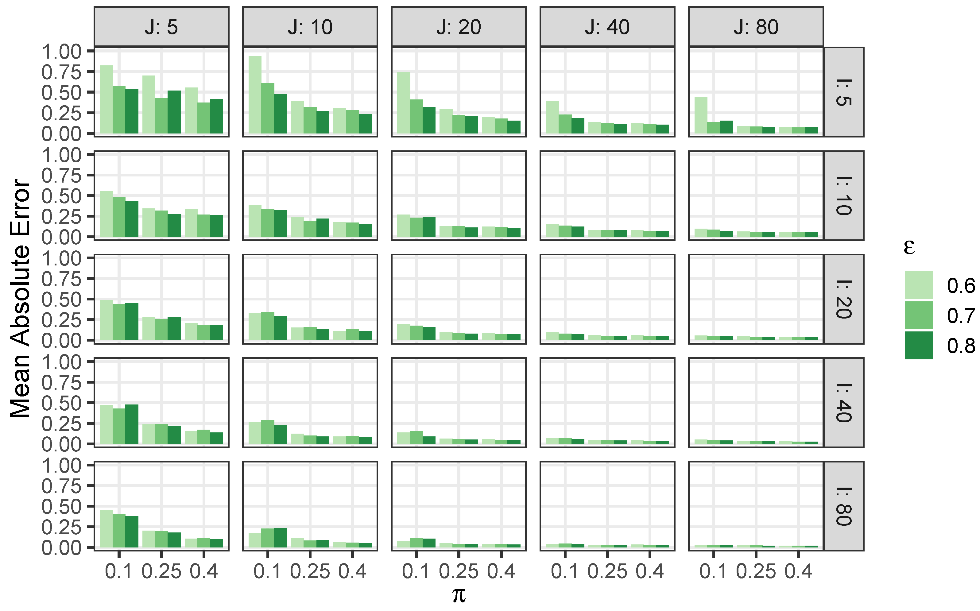
| J = 5 | J = 10 | J = 20 | J = 40 | J = 80 | |||||||||||||
|---|---|---|---|---|---|---|---|---|---|---|---|---|---|---|---|---|---|
| 0.1 | 0.25 | 0.4 | 0.1 | 0.25 | 0.4 | 0.1 | 0.25 | 0.4 | 0.1 | 0.25 | 0.4 | 0.1 | 0.25 | 0.4 | |||
| 0.6 | 0.82 | 0.70 | 0.55 | 0.94 | 0.39 | 0.30 | 0.75 | 0.29 | 0.19 | 0.39 | 0.14 | 0.12 | 0.44 | 0.09 | 0.08 | ||
| 0.7 | 0.57 | 0.43 | 0.37 | 0.61 | 0.32 | 0.28 | 0.41 | 0.22 | 0.18 | 0.23 | 0.12 | 0.11 | 0.14 | 0.08 | 0.07 | ||
| 0.8 | 0.54 | 0.52 | 0.42 | 0.47 | 0.27 | 0.23 | 0.31 | 0.21 | 0.15 | 0.18 | 0.11 | 0.10 | 0.15 | 0.08 | 0.07 | ||
| 0.6 | 0.55 | 0.34 | 0.33 | 0.38 | 0.24 | 0.18 | 0.27 | 0.13 | 0.12 | 0.15 | 0.08 | 0.08 | 0.10 | 0.06 | 0.06 | ||
| 0.7 | 0.48 | 0.32 | 0.27 | 0.34 | 0.19 | 0.17 | 0.23 | 0.13 | 0.12 | 0.13 | 0.08 | 0.07 | 0.09 | 0.06 | 0.05 | ||
| 0.8 | 0.43 | 0.27 | 0.26 | 0.32 | 0.22 | 0.15 | 0.24 | 0.11 | 0.10 | 0.12 | 0.08 | 0.07 | 0.07 | 0.05 | 0.05 | ||
| 0.6 | 0.49 | 0.28 | 0.21 | 0.33 | 0.15 | 0.12 | 0.20 | 0.09 | 0.08 | 0.10 | 0.06 | 0.06 | 0.06 | 0.05 | 0.04 | ||
| 0.7 | 0.44 | 0.26 | 0.19 | 0.35 | 0.16 | 0.13 | 0.18 | 0.09 | 0.08 | 0.08 | 0.05 | 0.05 | 0.05 | 0.04 | 0.04 | ||
| 0.8 | 0.45 | 0.28 | 0.18 | 0.30 | 0.13 | 0.11 | 0.16 | 0.08 | 0.07 | 0.07 | 0.05 | 0.05 | 0.05 | 0.04 | 0.04 | ||
| 0.6 | 0.47 | 0.24 | 0.15 | 0.26 | 0.12 | 0.09 | 0.14 | 0.06 | 0.06 | 0.07 | 0.04 | 0.04 | 0.05 | 0.03 | 0.03 | ||
| 0.7 | 0.43 | 0.24 | 0.17 | 0.29 | 0.10 | 0.09 | 0.15 | 0.06 | 0.05 | 0.07 | 0.04 | 0.04 | 0.05 | 0.03 | 0.03 | ||
| 0.8 | 0.48 | 0.22 | 0.14 | 0.23 | 0.09 | 0.08 | 0.09 | 0.05 | 0.04 | 0.06 | 0.04 | 0.04 | 0.04 | 0.03 | 0.02 | ||
| 0.6 | 0.45 | 0.20 | 0.11 | 0.17 | 0.11 | 0.06 | 0.08 | 0.05 | 0.04 | 0.04 | 0.03 | 0.03 | 0.03 | 0.02 | 0.02 | ||
| 0.7 | 0.41 | 0.19 | 0.12 | 0.23 | 0.08 | 0.05 | 0.11 | 0.04 | 0.04 | 0.04 | 0.03 | 0.03 | 0.03 | 0.02 | 0.02 | ||
| 0.8 | 0.38 | 0.18 | 0.10 | 0.23 | 0.09 | 0.05 | 0.11 | 0.04 | 0.03 | 0.04 | 0.03 | 0.03 | 0.03 | 0.02 | 0.02 | ||
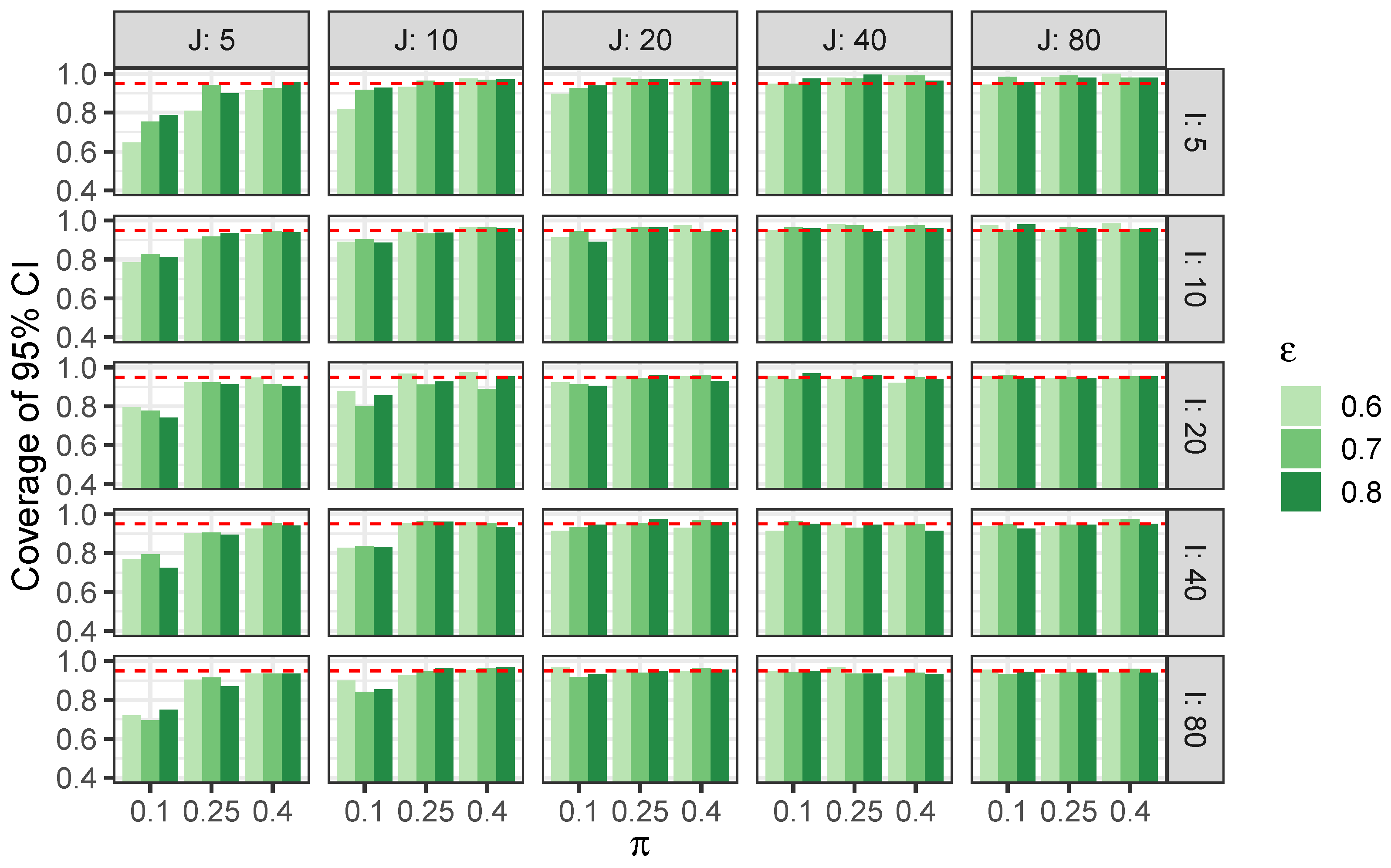
| J = 5 | J = 10 | J = 20 | J = 40 | J = 80 | |||||||||||||
|---|---|---|---|---|---|---|---|---|---|---|---|---|---|---|---|---|---|
| 0.1 | 0.25 | 0.4 | 0.1 | 0.25 | 0.4 | 0.1 | 0.25 | 0.4 | 0.1 | 0.25 | 0.4 | 0.1 | 0.25 | 0.4 | |||
| 0.6 | 0.65 | 0.81 | 0.92 | 0.82 | 0.93 | 0.97 | 0.90 | 0.98 | 0.97 | 0.95 | 0.98 | 0.99 | 0.94 | 0.98 | 1.00 | ||
| 0.7 | 0.75 | 0.94 | 0.93 | 0.92 | 0.96 | 0.97 | 0.93 | 0.97 | 0.97 | 0.95 | 0.98 | 0.99 | 0.98 | 0.99 | 0.98 | ||
| 0.8 | 0.79 | 0.90 | 0.96 | 0.93 | 0.96 | 0.97 | 0.94 | 0.97 | 0.96 | 0.97 | 1.00 | 0.96 | 0.96 | 0.98 | 0.98 | ||
| 0.6 | 0.79 | 0.91 | 0.93 | 0.89 | 0.94 | 0.96 | 0.91 | 0.96 | 0.98 | 0.95 | 0.98 | 0.97 | 0.98 | 0.95 | 0.98 | ||
| 0.7 | 0.83 | 0.92 | 0.95 | 0.90 | 0.93 | 0.96 | 0.95 | 0.96 | 0.94 | 0.96 | 0.98 | 0.98 | 0.95 | 0.96 | 0.96 | ||
| 0.8 | 0.81 | 0.94 | 0.94 | 0.89 | 0.94 | 0.96 | 0.89 | 0.96 | 0.95 | 0.96 | 0.94 | 0.96 | 0.98 | 0.96 | 0.96 | ||
| 0.6 | 0.80 | 0.92 | 0.95 | 0.88 | 0.97 | 0.98 | 0.92 | 0.95 | 0.96 | 0.96 | 0.94 | 0.92 | 0.96 | 0.94 | 0.94 | ||
| 0.7 | 0.78 | 0.92 | 0.91 | 0.80 | 0.91 | 0.89 | 0.91 | 0.94 | 0.96 | 0.94 | 0.95 | 0.95 | 0.96 | 0.95 | 0.96 | ||
| 0.8 | 0.74 | 0.91 | 0.90 | 0.86 | 0.93 | 0.95 | 0.90 | 0.96 | 0.93 | 0.97 | 0.96 | 0.94 | 0.94 | 0.94 | 0.96 | ||
| 0.6 | 0.77 | 0.90 | 0.93 | 0.83 | 0.95 | 0.96 | 0.91 | 0.95 | 0.93 | 0.91 | 0.95 | 0.94 | 0.94 | 0.94 | 0.98 | ||
| 0.7 | 0.79 | 0.91 | 0.95 | 0.84 | 0.96 | 0.95 | 0.93 | 0.96 | 0.97 | 0.96 | 0.93 | 0.95 | 0.95 | 0.94 | 0.98 | ||
| 0.8 | 0.73 | 0.89 | 0.94 | 0.83 | 0.96 | 0.93 | 0.95 | 0.98 | 0.96 | 0.95 | 0.94 | 0.92 | 0.92 | 0.94 | 0.95 | ||
| 0.6 | 0.72 | 0.90 | 0.94 | 0.90 | 0.93 | 0.95 | 0.97 | 0.95 | 0.95 | 0.95 | 0.97 | 0.92 | 0.96 | 0.93 | 0.94 | ||
| 0.7 | 0.70 | 0.91 | 0.94 | 0.84 | 0.95 | 0.96 | 0.92 | 0.94 | 0.96 | 0.94 | 0.94 | 0.94 | 0.93 | 0.94 | 0.96 | ||
| 0.8 | 0.75 | 0.87 | 0.94 | 0.86 | 0.96 | 0.97 | 0.93 | 0.95 | 0.96 | 0.95 | 0.94 | 0.93 | 0.94 | 0.94 | 0.94 | ||
Appendix C.2. Additional Results from Section 5.2
| Parameter | (95% CI) | ||||||||||
|---|---|---|---|---|---|---|---|---|---|---|---|
| Estimate | 0.25 | 0.88 | 50.55 | 13.84 | 3.65 (3.22, 4.08) | ||||||
| Site (i) | 1 | 2 | 3 | 4 | 5 | 6 | 7 | 8 | 9 | 10 | 11 |
| 0.104 | 0.166 | 0.065 | 0.261 | 0.293 | 0.366 | 3.413 | 2.574 | 1.434 | 4.485 | 0.116 |
References
- Baker, G.B.; Holdsworth, M. Seabird monitoring study at Coringa Herald National Nature Reserve 2012; Report Prepared for Department of Sustainability, Environment, Water, Populations and Communities; Latitude 42 Environmental Consultants Pty Ltd.: Kettering, TAS, Australia, 2013. [Google Scholar]
- Bouveyron; Celeux, C.G.; Murphy, T.B.; Raftery, A.E. Model-Based Clustering and Classification for Data Science: With Applications in R; Cambridge University Press: Cambridge, UK, 2019. [Google Scholar]
- Lindsay, B.G. Mixture Models: Theory, Geometry, and Applications; Institute for Mathematical Statistics: Hayward, CA, USA, 1995. [Google Scholar]
- McLachlan, G.J.; Peel, D. Finite Mixture Models; Wiley: New York, NY, USA, 2000. [Google Scholar]
- Martin, T.G.; Wintle, B.A.; Rhodes, J.R.; Kuhnert, P.M.; Field, S.A.; Low-Choy, S.J.; Tyre, A.J.; Possingham, H.P. Zero tolerance ecology: Improving ecological inference by modelling the source of zero observations. Ecol. Lett. 2005, 8, 1235–1246. [Google Scholar] [CrossRef] [PubMed]
- Lambert, D. Zero-inflated Poisson regression, with an application to defects in manufacturing. Technometrics 1992, 34, 1–14. [Google Scholar] [CrossRef]
- Lim, H.K.; Li, W.K.; Philip, L.H. Zero-inflated Poisson regression mixture model. Comput. Stat. Data Anal. 2014, 71, 151–158. [Google Scholar] [CrossRef]
- Long, D.L.; Preisser, J.S.; Herring, A.H.; Golin, C.E. A marginalized zero-inflated Poisson regression model with overall exposure effects. Stat. Med. 2014, 33, 5151–5165. [Google Scholar] [CrossRef] [PubMed]
- Jamshidian, M.; Jennrich, R.I. Standard errors for EM estimation. J. R. Stat. Soc. Ser. B 2000, 62, 257–270. [Google Scholar] [CrossRef]
- Aitken, M.; Rubin, D.B. Estimation and hypothesis testing in finite mixture models. J. R. Stat. Soc. Ser. B 1985, 47, 67–75. [Google Scholar] [CrossRef]
- McLachlan, G.J.; Krishnan, T. The EM Algorithms and its Extensions, 2nd ed.; Wiley: New York, NY, USA, 2008. [Google Scholar]
- Hoadley, B. Asymptotic properties of maximum likelihood estimators for the independent not identically distributed case. Ann. Math. Stat. 1971, 42, 1977–1991. [Google Scholar] [CrossRef]
- Efron, B.; Hinkley, D.V. Assessing the accuracy of the maximum likelihood estimator: Observed versus expected Fisher information. Biometrika 1978, 65, 457–482. [Google Scholar] [CrossRef]
- Louis, T. Finding the observed information matrix when using the EM Algorithm. J. R. Stat. Soc. Ser. B 1982, 44, 226–233. [Google Scholar] [CrossRef]
- Johnson, N.L.; Kemp, A.W.; Kotz, S. Univariate Discrete Distributions, 3rd ed.; Wiley-Interscience: Hoboken, NJ, USA, 2005. [Google Scholar]
| Frigatebird Subspecies | Nest Counts | Relative Proportion |
|---|---|---|
| Lesser | 46 | 0.036 |
| Greater | 81 | 0.063 |
| Unidentified | 1158 | 0.901 |
| Site | August 2007 | September 2008 | October 2009 | August 2012 |
|---|---|---|---|---|
| 1 | 0 | 1 | 0 | 3 |
| 2 | 2 | 0 | 8 | 4 |
| 3 | 1 | 1 | 2 | 2 |
| 4 | 4 | 4 | 14 | 2 |
| 5 | 12 | 1 | 8 | 6 |
| 6 | 0 | 0 | 18 | 6 |
| 7 | 54 | 0 | 209 | 4 |
| 8 | 53 | 54 | 127 | 3 |
| 9 | 24 | 3 | 80 | 25 |
| 10 | 137 | 62 | 196 | 18 |
| 11 | 4 | 2 | 4 | 0 |
| Parameter | (95% CI) | ||||
|---|---|---|---|---|---|
| Estimate | 0.25 | 0.84 | 66.60 | 18.22 | 3.65 (3.23, 4.08) |
Disclaimer/Publisher’s Note: The statements, opinions and data contained in all publications are solely those of the individual author(s) and contributor(s) and not of MDPI and/or the editor(s). MDPI and/or the editor(s) disclaim responsibility for any injury to people or property resulting from any ideas, methods, instructions or products referred to in the content. |
© 2025 by the authors. Licensee MDPI, Basel, Switzerland. This article is an open access article distributed under the terms and conditions of the Creative Commons Attribution (CC BY) license (https://creativecommons.org/licenses/by/4.0/).
Share and Cite
Pearce, M.; Perlman, M.D. Estimating the Ratio of Means in a Zero-Inflated Poisson Mixture Model. Stats 2025, 8, 55. https://doi.org/10.3390/stats8030055
Pearce M, Perlman MD. Estimating the Ratio of Means in a Zero-Inflated Poisson Mixture Model. Stats. 2025; 8(3):55. https://doi.org/10.3390/stats8030055
Chicago/Turabian StylePearce, Michael, and Michael D. Perlman. 2025. "Estimating the Ratio of Means in a Zero-Inflated Poisson Mixture Model" Stats 8, no. 3: 55. https://doi.org/10.3390/stats8030055
APA StylePearce, M., & Perlman, M. D. (2025). Estimating the Ratio of Means in a Zero-Inflated Poisson Mixture Model. Stats, 8(3), 55. https://doi.org/10.3390/stats8030055