1. Introduction
The phenomenon of noise-induced transport has attracted (and still attracts) a lot of interest (see Refs. [
1,
2,
3]). Noise-induced transport is the directed transport of matter emerging in a stochastic system with a periodic potential. Such transport can occur even in the absence of a directed external force. Starting from the pioneering work found in Refs. [
4,
5], active theoretical and numerical investigations of such model systems with asymmetric potential (“ratchets”) were stimulated by their potential ability to explain the functionality of motor proteins responsible for the motion of cells. In the pioneering works and the references found therein, one finds a theoretical analysis of the current induced by chaotic noise, as well as the physical essence of the emergence of the current reversal compared to the “traditional” stochastic process. The kangaroo process, the importance of the flatness, as well as the idea of the current reversals, were introduced in Refs. [
6,
7,
8,
9]. However, the applicability of the concept is much wider. Several experimental groups have found confirmation of Brownian movement in chemical systems (directed diffusion [
9,
10] or rotation [
11,
12] of molecules), highlighting possible applications of the “ratchet effect” in nanoscale mechanical devices and separation techniques. Various ratchet-like mechanisms have been intensively studied, including an analysis of sources of driven (deterministic and/or random) forces or potentials, the statistics of non-thermal fluctuations, conditions for optimal transport, etc. [
13,
14]. The subject has become attractive for at least two reasons—the possibility of a satisfactory explanation of the directed motion of molecular motors, which transport macromolecules in biological cells [
15,
16], and attempts to construct well-controlled high-resolution devices for the separation of macro-particles or micro-objects such as cells, viruses, DNA, or proteins [
17,
18,
19,
20,
21,
22,
23]. “Ratchets” has been applied to the study of various physical systems, from chemical reactions and ring-laser gyroscopes to neural networks. A good review of physical applications can be found in Ref. [
24]. Under stochastic stimulus, the model demonstrates numerous interesting phenomena, including stochastic resonance and noise-induced transport [
25,
26,
27,
28,
29,
30,
31,
32,
33]. For more recent developments in this area, cf. e.g., Refs. [
34,
35,
36].
This present work investigates Brownian motion in a correlation ratchet with a sawtooth potential, driven by additive (thermal) Gaussian white noise and additive colored noise, namely trichotomous noise. Although both kinds of noise have zero mean, the system exhibits directed motion, i.e., the Brownian particle will preferentially move in one direction, expressed by a current,
J. Moreover, the direction of this current depends on parameters such as the diffusion constant of the Brownian motion, implying that this setup is useful for the separation of particles with different friction coefficients. For the average particle’s current,
J, the authors drew conclusions from a graphical analysis [
30,
31,
32,
33]. A new effect of three current reversals as a function of noise amplitude was discovered. The area of validity of this effect turned out to be very large, to the advantage of the effects caused by it. A system of equations describing the multiple current reversals effect was derived; it was shown that if an arbitrary model has
p variables, no more than
p-fold critical points are present, with
p being an indicator of the corresponding multiplicity of current reversals. The disjunct window as a function of temperature and switching rate as control parameters is discussed. Finally, the deterministic noise-induced transport of overdamped Brownian particles in a ratchet system is considered. The simplicity of the exact solution and the model itself is beneficial for a possible experiment. A hypersensitive response to the variation of almost all system parameters is observed. In particular, this effect is useful for separating substances that are inseparable by conventional means.
2. The Model
The overdamped motion of Brownian particles is described by the dimensionless Langevin equation
where
,
is a spatial potential with period
, and
is the barrier height. Equation (
1) corresponds to Newton’s Second Law of Mechanics. Here, the word “overdamped” means that the acceleration
is taken to be zero. This approximation is usable in models with friction (for example, a parachutist falling with constant velocity). The usual physical variables are indicated by tildes. In the dimensionless form, the space and time coordinates read
and
, where
is the friction coefficient.
Thermal noise satisfies
with
. For brevity, in what follows, we shall denote
D as the temperature. Concerning the random force
, this is assumed to be created by a zero-mean trichotomous Markovian stochastic process [
28,
29,
30,
31,
32,
33], consisting of jumps between three values,
, with
. The jumps follow in time according to a Poisson process, while the values occur with the stationary probabilities
and
. In a stationary state, the fluctuation process satisfies
where the switching rate
is the reciprocal of the noise correlation time
, i.e.,
is a symmetric zero-mean exponentially correlated noise. The trichotomous process is a particular case of the kangaroo process [
37] with flatness parameter
.
To derive an exact formula for the stationary current
of particles, it is assumed that the potential
in Equation (
1) with
is piecewise linear (sawtooth-like) with asymmetry determined by a parameter
, where
is symmetric for
. The force corresponding to the potential is
for
and
for
. Under these assumptions, a closed-form expression for the probability current
J was derived in Equation (27) of Ref. [
28].
J can be presented as a quotient of two eleventh-order determinants in Equation (14) of Ref. [
29].
To obtain a more treatable explicit formula, one can assume that the flatness parameter
is large, and expand the current in a series in
q,
. An exact (but still complex) formula for the leading order term
was derived in Equation (31). Since the present article is restricted to the case of
q close to zero, the current can be assumed to be small as well. By direct numerical calculations, it can be shown that the effects reported in this paper are present at least up to
. Indeed, the simplification of the equations via expansion in
q preserves the main effects. Because of this, the ratchet model is also relevant for biological systems; allowing one to find the most narrow condition (cf.
Figure 1) is one way to understand the biological stochastic transport.
3. Multiple Current Reversals
A current reversal (CR) is defined as the sign change of a current
at a particular value of one of the parameters (
a), with the remaining parameters fixed. For certain parameter values, there exist three CRs, as opposed to two CRs in most of the previous models. The multiple current reversals phenomenon is considered to be “one of the most interesting aspects of the theory of Brownian ratchets” [
38], and “more detailed analytical predictions are invaluable” [
23]. The multiple current reversals effect has been studied in detail in Ref. [
39].
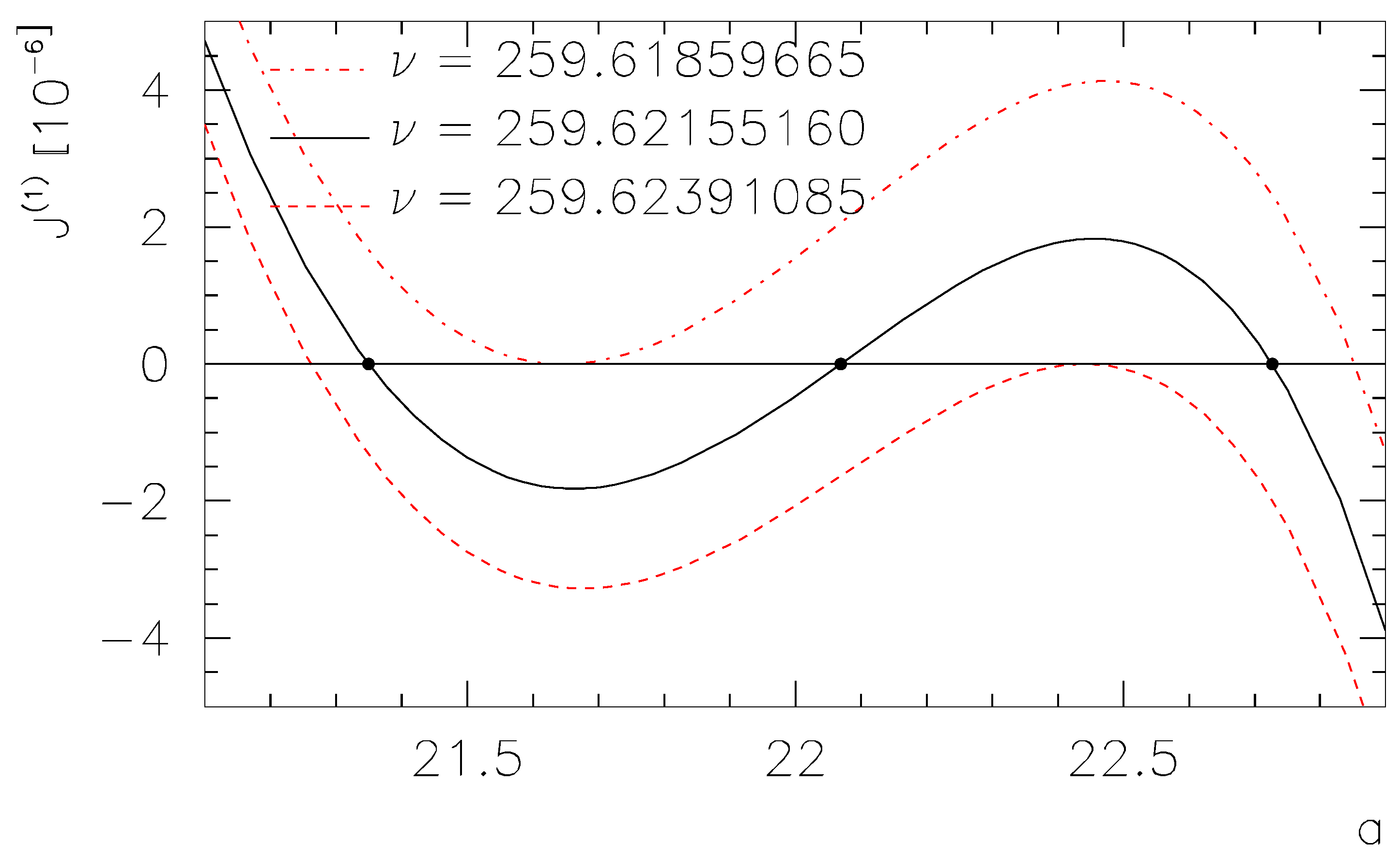
In order to discuss the 3CR effect,
Figure 2 exhibits the three zeros of the current. By gradually varying system parameters, one obtains the surprising result that the region of the 3CR effect vs. amplitude effect is extremely large [
30,
31,
32,
33].
The necessary conditions for the existence of the 3CR effect are shown in
Figure 3a by the shaded regions in the planes
and
, while the shaded, sail-shaped areas in
Figure 3b fix the values of
and
, which are necessary and sufficient for the existence of the 3CR effect as a function of
a. For instance, for
it is necessary that
. This formula is an interpolation of the upper edge of the
“sail”, with the latter being produced numerically from the formula for the current in the paper by Mankin. Within the interval
, the error is below 5 percent. Accordingly, for
, it is necessary that
(within
, the error does not exceed 2 percent).
In
Figure 2, curve 2 has three CR points at positions
. Let us consider a general case with
n zeros of the current in dependence on some system parameter
a, namely
for
, assuming
. Because the function
must have (at least)
extrema between the
n CR points, the first derivative has
zeros and, as a consequence,
extrema. This scheme continues up to the
-th order derivative. In conclusion, the current and the derivatives up to order
have zeros between
and
. We define the
critical position (in the parameter space) as the position where all
n CR points are “gathered” to the same spot, namely
for
. For the multiple CR effect, the (yet unreported) “
n-fold zero critical position” is a solution to the system:
From the number of independent equations and independent variables in the system (
3), it follows that if the model has
p independent parameters, the possible foldedness is limited to
. Since Equation (
3) discloses the critical points, it also describes the conditions for the existence of multiple CR effects. For instance, the edges of the “sails” in
Figure 3b are “2-fold critical points”, like in
Figure 2 for curves 1 and 3, while the sharp peaks of the “sails” are 3-fold critical points.
The difference in multiplicity, like 2CR and 3 CR, is essential. When talking about multiple CRs, 2CR is the quietly accepted standard. Hopefully, studying the next level (3CR) will disclose additional prospects for applying ratchet models to describe various processes in biology, nanotechnology, sociology, etc. For example, while the 2CR effect allows only one pair of motor proteins to move simultaneously in opposite directions along the microtubules inside eukaryotic cells, the 3CR effect allows such simultaneous motion of two pairs of motor proteins.
4. Disjunct Windows
Returning to the particular model in Equation (
1), “disjunct windows” (DWs) are defined as closed curves of the solution
in the plane
[
30,
31,
32,
33].
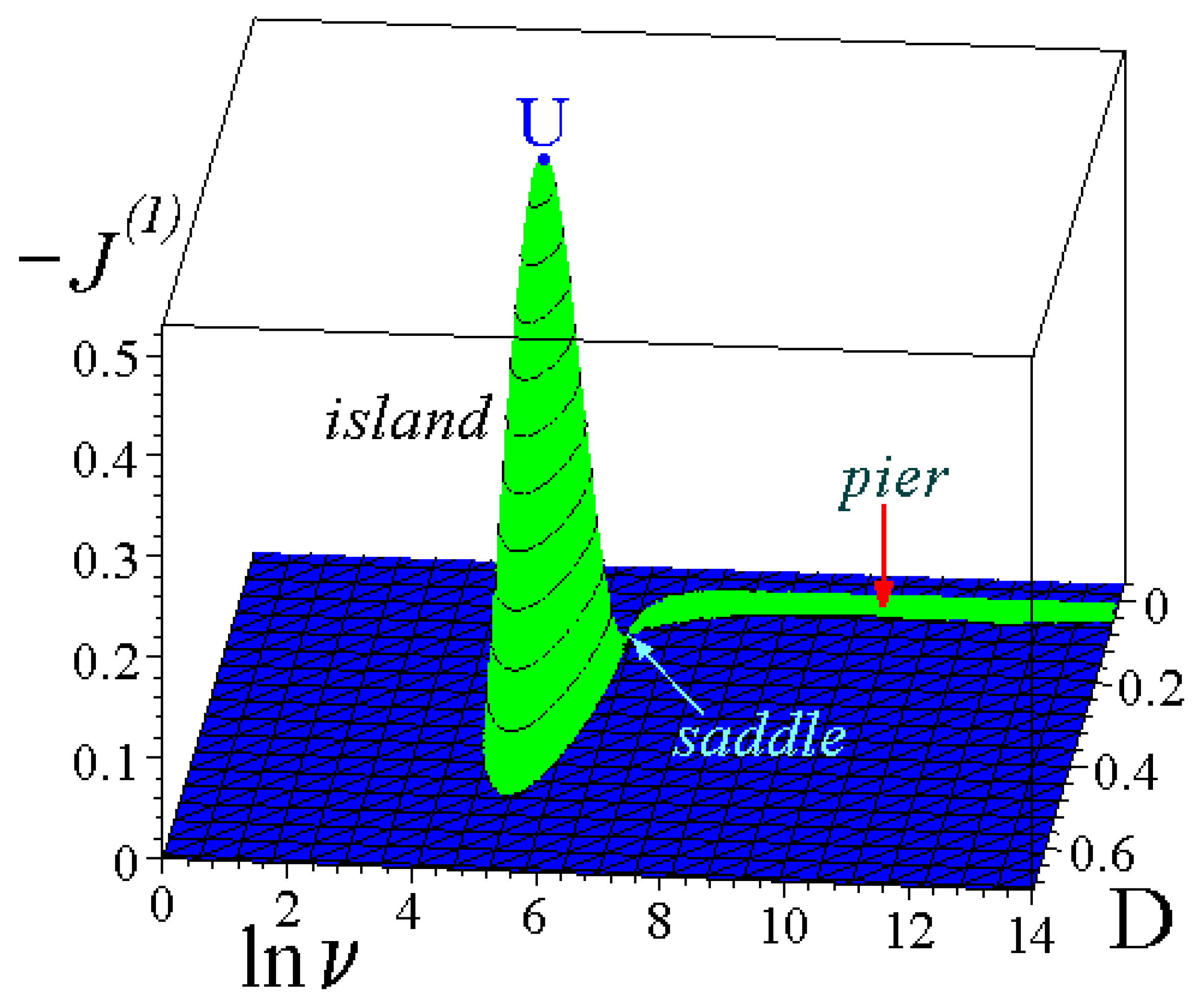
Figure 1 shows two windows (an island and a pier-like window) with negative current in the plane
. The “island” has a narrow peak for the current and, consequently, the quality of the separation of the substance is maximal there.
Incomparably more information relevant to the existence condition of disjunct windows than that in Refs. [
30,
31,
32,
33] is presented in
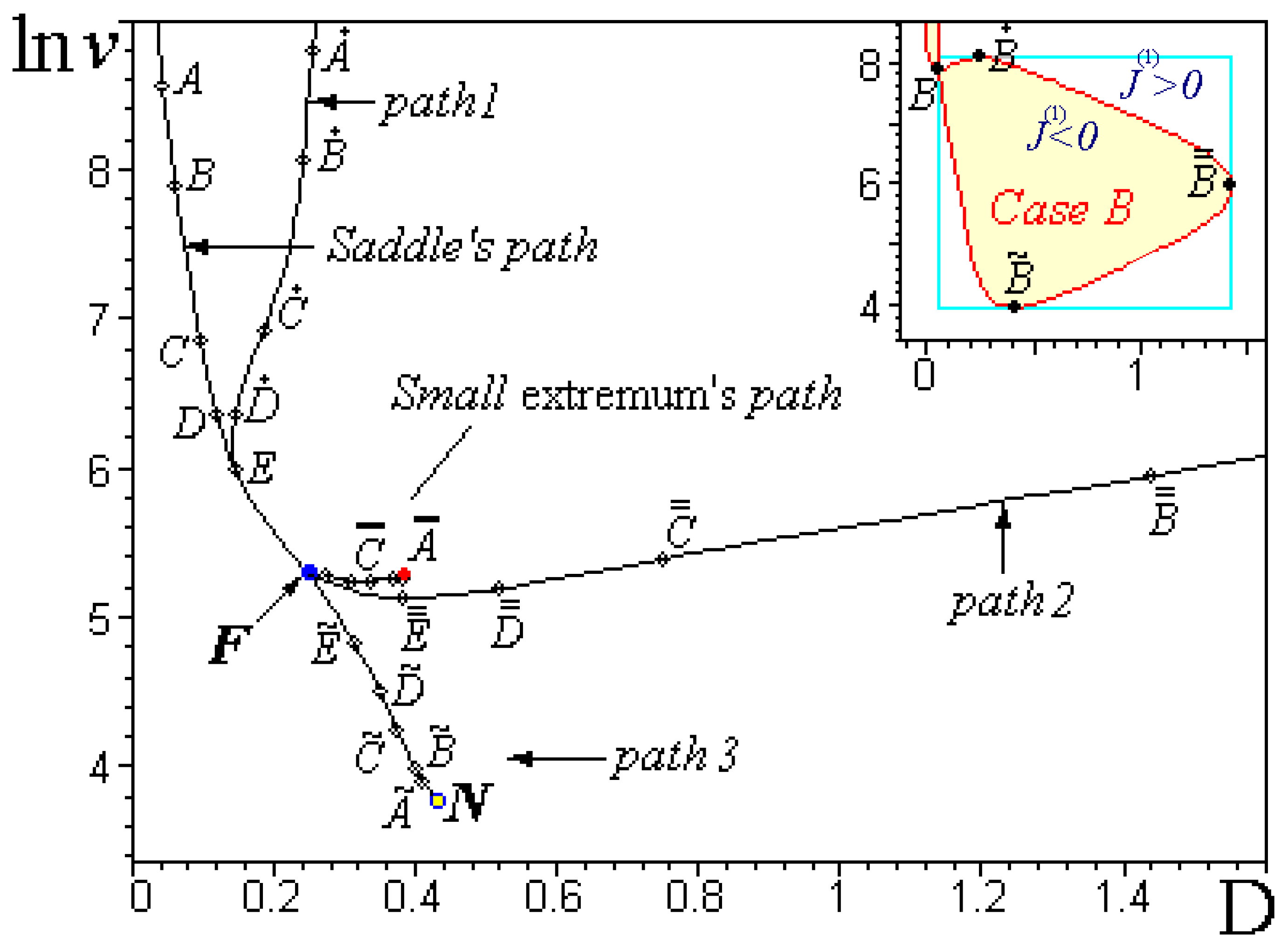
Figure 4. The picture shows critical points in the plane
describing the “island” window. The extrema and saddle paths represent pairs of solutions of the boundary
of the island for either
or
, cf. the inlet of
Figure 1. As there are three equations but four independent variables, the solutions are functions (say, of the asymmetry
). Namely, the “extremum” has
,
, and
, while the “saddle” has
,
, and
. Here, and in the following, the label
x denotes the value of the “extremum”, while the label
s stands for the “saddle”. In this way, one obtains “path 1” and “path 3” by solving
and
, and “path 3” and “saddle’s path” by solving
and
. For a fixed value of
a in the interval
, these solutions form a “box”
,
in the plane
, where the labels
,
, and
correspond to “paths” 1, 2, and 3. The “case B” example plotted in the inlet of
Figure 1 is defined by the asymmetry parameter
.
Only “path 3” and the “small extremum’s path” have finite lengths. Note that the “small extremum’s path” (the appearance of the “island”) is well localized within the ranges , and .
From the literature, as well as from the present model, it is known that outside the region of the DWs, the two zeros of the current
(i.e., 2CRs) generally occur at largely displaced values of
(cf. the “pier” area in
Figure 1). Therefore, particles whose friction coefficients are within a wide interval move in the negative direction, and the separation effect is of low selectivity. Although this wide interval can be made narrower by varying the other system parameters, the really narrow intervals were realized only in the vicinity of the transition regimes (i.e., in the transition from two CRs to zero CR), where the absolute value of the current is small. On the other hand, in the DWs, the negative current
has a sharp extremum in a relatively narrow region where the absolute value of the current is large (cf.
Figure 1). By adjusting the temperature within a window, one can easily achieve the maximal absolute value of the current for particles with selected friction coefficients.
The relatively large absolute value of the current in DWs can be partly explained by the fact that DWs occur at relatively small
. As a rule, increasing the switching rate
entails a decrease in the absolute value of the extrema of the currents; if the intensity of the thermal noise dominates (
), the current becomes small due to the second law of thermodynamics. Indeed, the asymptotics give
for
,
,
, or
[
28,
29].
It is our hope that the new effects found are realized within the regions of parameters that are relevant to cell biology. The exact knowledge of the whereabouts of the effects will greatly facilitate their application in theoretical models as well as in the design of separation devices. Aiming to find optimal regimes for the system (temperature
D, signal frequency
, amplitude
a, etc.) makes the device more profitable. For example, the effect of 3CR in
Figure 3 could be used with moderate temperatures and frequencies like
and
, but only in devices with
.
5. An Analytically Solvable Model
In Refs. [
30,
31,
33], one of the authors demonstrated that the CR effect is attainable in various ways, e.g., variations in the temperature (up to 4 CRs) and the correlation time (up to 6 CRs) of nonequilibrium fluctuations.
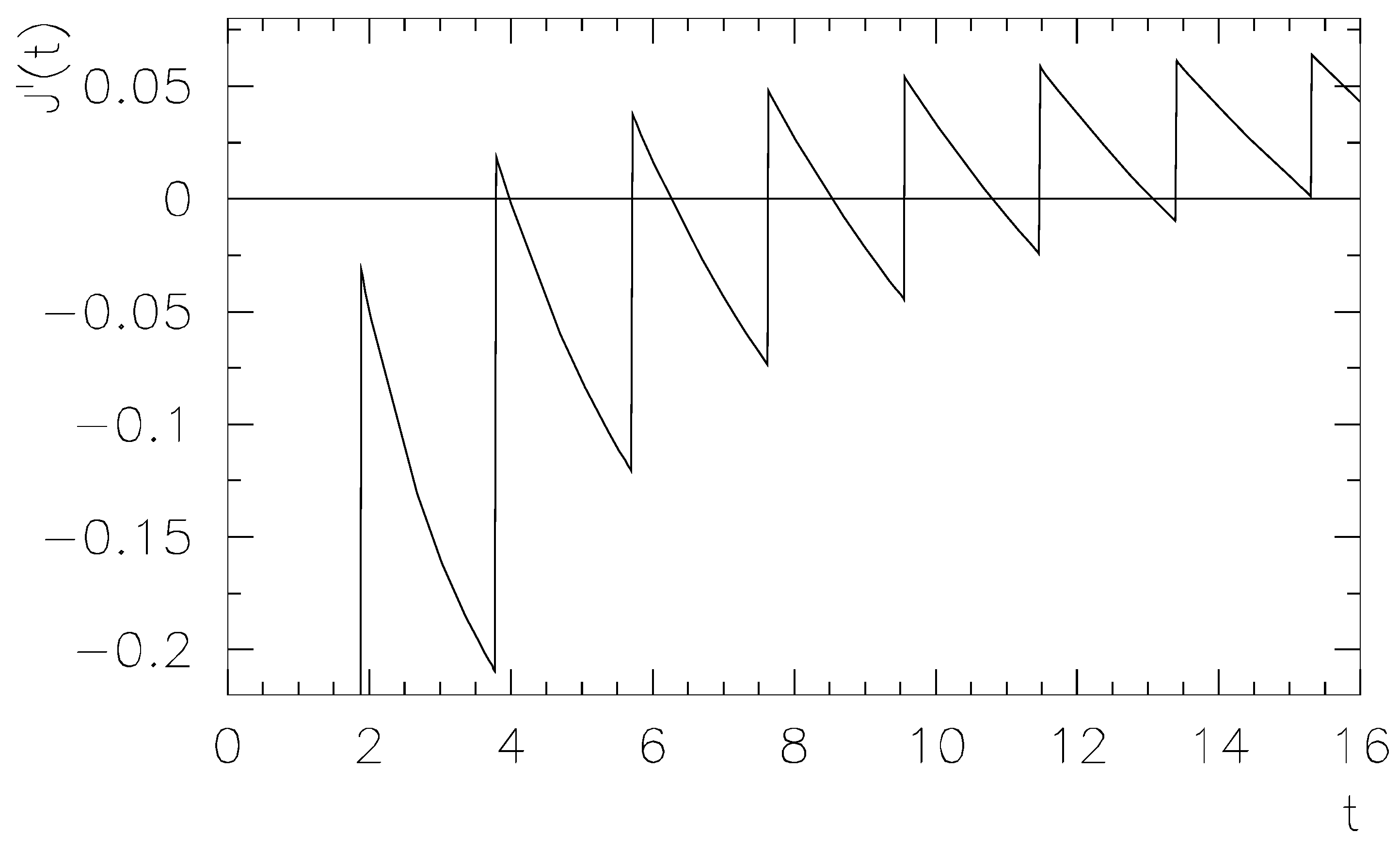
Figure 5 exhibits 11 CRs. To the knowledge of the authors, more than six CRs have never been reported for ratchets with a simple sawtooth potential. As the difference in multiplicity is essential, this is one aspect that the model presented here can offer. Another aspect is hypersensitivity. The phenomenon of hypersensitivity can be defined as a drastic (abrupt) change in the current resulting from infinitesimally small variations in (some of) the model’s parameters. This effect could be used for signal amplification in technological devices. As advised in Ref. [
40], the phenomenon may also shed some light on the ability of biological systems to detect weak signals. The effect has been the topic of several physical investigations, cf. e.g., Refs. [
32,
41,
42,
43,
44,
45,
46,
47].
A model with hypersensitivity has discontinuities in the current (let us call them “jumps”) as a function of at least one of the parameters. That effect could be useful for the amplification of weak signals, but to the authors’ knowledge, the following application has never been explicitly formulated: hypersensitivity could segregate different nano-objects (e.g., virus or DNA) from a suspension even if their parameters are almost indistinguishable.
Indeed, if one object has
and the other
, where
is constant and
a small difference, one can define a
separation quality as the difference in current values,
The quality,
Q, is zero unless
is at a position of discontinuity.
Separation is understood as the increasing spatial gap between different objects, e.g.,
. The impression is that a model with a sharp potential and dichotomous noise does not exhibit hypersensitivity [
32]. However, the following model is an exception to this.
The system is described by the dimensionless Langevin equation:
where
is the force corresponding to a piecewise linear, sawtooth-like potential, as given by Equation (
1). This time, however, one uses deterministic noise
, which is periodic and dichotomous,
with
, where
is the rational part of
x, e.g.,
. The physical motivation for
is a technical device for the separation of substances, which would have effects such as, for instance, multiple hypersensitivity. Here,
t and
k are positive constants, describing the durations of the noise values
and
in each of the periods, respectively. If
, the current is blocked, and the particle can be in motion no longer than
If
, moving from
to
takes the time
but passing from
to
in total takes the time
Visualizing the motion of a particle under the above conditions in
Figure 6 gives the solution
where
is the integer part of
x, e.g.,
. The condition
for the constant
k (see Equation (
7)) ensures that the particle moving to the left reaches the minimum of the potential, enabling an analytical instead of a numerical calculation. The averaging procedure is analytical, since the noise is deterministic.
Figure 6 shows the device with spatial dimension
x under the action of an (integrated) field
that acts deterministically on the Brownian particle. One can see the motion in Ref. [
48], where this particle starts to move to the right with an averaged velocity
J.
Obviously, jumps in Equation (
10) occur when the argument of the operator
U becomes
Because this condition (
11) depends on variables
a,
t, and
d, the curves
,
, and
(with the other parameters fixed) have plenty of discontinuities. The depth of each discontinuity
is the quality of separation, see Equation (
4). The deepest jump has
for
,
,
, and
. To our knowledge, this is the largest number found up to now. Ref. [
32] provides only
.
As the period
is reciprocal to the friction
[
30,
31,
32,
33], it means that the jump can occur at a particular value of
by adjusting the period
of the signal in order to separate particles with different frictions.
6. Frame Method
The frame method explains why the model allows for multiple CRs. In order to explain this frame method, we will provide a practical (macroscopic) example. Suppose the long, narrow pipe along the highway from New York to Boston is maintained, and suppose that this pipe contains a periodic potential acting on Brownian particles. Suppose that particles with friction move with speed . Suppose that other particles with move with , and a third group of particles with moves with . As you see, the function does not have any current reversals. Now, a tester starts to walk along this highway from New York to Boston. His speed is constant and equals . Relative to this observer, the speed of the first group of particles (those with ) will become . Particles move to the left, i.e., in the direction of New York. But the speed of the second group of particles will be . Therefore, these particles move to the right, i.e., in the direction of Boston. This means that the function now has a current reversal at about . As the particles of the third group have the speed , the function has a second current reversal at about . Therefore, the frame method can be considered as a mechanism to increase the multiplicity of current reversals (in this example, from 0CR to 2CR) just because the function is nonmonotonic. This function is the solution of the nonmonotonic master equation of the concrete stochastic system. Without this nonmonotonicity, of course, one cannot increase the number of current reversals from 0 to 2.
Returning to the model, in Equation (
10), there is no CR effect. However, in a coordinate system that moves along
x with velocity
v (with respect to the potential), the current is
with
J from Equation (
10), and a CR effect is always possible. For some range of parameter values of
v, there exist multiple current reversals, like the eleven CRs in
Figure 5. The phenomenon could be called “multiple hypersensitive CRs”, as the current jumps repeatedly from a negative to a positive value with an infinite derivative.
The speed
in
Figure 5 is the speed of the potential relative to the observer. This means that the particle flow seen by the observer is given by Equation (
12). Since according to
J in Equation (
10) the Brownian particle changes its direction of motion, the shift to the right shown in Ref. [
48] is indeed slower than it would be in some simpler model. However, the periodic change of the direction of motion is necessary to cause hypersensitive jumps in
Figure 5 for small changes in some of the parameters like
t. The jumps are needed to separate different substances from a mixture, as discussed in Equation (
4).
Apart from the amplification of weak signals (when the transition is made smoother by adjusting the temperature) and separation, the model presented in this section could hopefully also be used in the design of certain types of detection devices. Geiger counters, biased Josephson junctions, and SQUIDs have the property that a very small perturbation can generate a large response [
23]. These detectors, as the model considered here, are nearly noiseless before the trigger event occurs, whereas systems with hypersensitivity are usually noisy structures to begin with.
