Abstract
Bayesian methods have attracted increasing interest in the design and analysis of clinical trials. Many of these clinical trials investigate time-to-event endpoints. The Weibull distribution is often used in survival and reliability analysis to model time-to-event data. We propose a process to elicit information about the parameters of the Weibull distribution for pharmaceutical applications. Our method is based on an expert’s answers to questions about the median and upper quartile of the distribution. Using the elicited information, a joint prior is constructed for the median and upper quartile of the Weibull distribution, which induces a joint prior distribution on the shape and rate parameters of the Weibull. To illustrate, we apply our elicitation methodology to a pediatric clinical trial, where information is elicited from a subject-matter expert for the control arm.
1. Introduction
The Weibull distribution is widely used in time-to-event analyses that arise in the fields of medicine, engineering, public health, and epidemiology [1,2]. While frequentist and Bayesian methods are both commonly used, the Bayesian approach is particularly useful in clinical trials when sample sizes are unavoidably small. This situation arises, for example, when the disease being investigated is rare, when clinical interest lies in monitoring a rare event of a common disease, or when there is a small patient subgroup [1]. Bayesian statistics can also be useful in clinical trials involving rare diseases, in which it may be difficult to reach the desired enrollment, as seen in pediatric clinical trials, where the pool of suitable subjects is limited [3].
Bayesian methods require the specification of a joint prior distribution on all unknown parameters. Using Bayes’ theorem, the joint prior is combined with a likelihood to yield posterior and posterior predictive distributions, which enable inference. The joint prior can be specified as being relatively non-informative when little prior information is available. Alternatively, an informative joint prior distribution can be constructed using historical data or expert opinion. Extraordinary care is always advised when using expert opinion, which may require questions to be asked in a familiar context on scales that can be transformed mathematically into priors for the parameters in the data model.
Elicitation is the process through which an expert’s knowledge and beliefs are used to construct a prior distribution for the parameter(s) of interest [4]. As noted, it is often advantageous for the elicitation to be focused on some observable quantity that is meaningful to the expert [5]. In a pharmaceutical setting, expert elicitation has been proven to increase the understanding of the potential study outcomes and the appreciation of the risks of the current study design [5]. There is an extensive literature on elicitation. Garthwaite et al. (2012) detailed the steps of the elicitation process, the heuristics and cognitive biases that a facilitator may encounter during an elicitation, methods to check the adequacy of the elicited prior, and strategies to manage group elicitations [6].
The elicitation process consists of four stages. The first stage includes selecting and training the expert(s) and identifying what quantities need to be elicited. Training experts is particularly important, as non-statisticians often confuse basic statistical quantities; however, it can be challenging due to resource constraints. In the second stage, specific summaries are elicited from the expert(s) using a series of questions. In stage three, a (joint) probability distribution is fitted to the elicited summaries. If multiple experts are involved, a method for combining opinions (or reconciling differences) must be used. In the fourth and final stage, the adequacy of the elicited prior distribution is assessed in terms of how well it represents the expert(s)’ opinion(s). If the resulting prior distribution is found to be inadequate, then the eliciting, fitting, and checking stages are performed again until a satisfactory representation of the expert(s)’ belief(s) is achieved. It is good practice to have a well-established framework when performing the elicitation process. Oakley and O’Hagan proposed a formal structure for the elicitation process, implemented in the SHeffield ELicitation Framework (SHELF) [7], and the elicitation of long-term survival outcomes has recently used that framework [8].
Extensive work has been carried out in the fields of survival and reliability analysis to elicit a joint prior for the parameters of the Weibull distribution. Some of these methods require elicitation directly on the parameters. Others require elicitation on potentially observable quantities that are then mathematically transformed to obtain information on the parameters. Some methods combine eliciting information on the parameters and observable quantities. In reliability analysis, when eliciting information for the Weibull distribution, it is common to elicit observable quantities to form a prior distribution for the scale parameter, while information about the shape parameter, which characterizes aging, is directly elicited [2,9,10,11]. The shape parameter is therefore easier to think about than the scale parameter [9]. In a clinical setting, biomedical experts may have little understanding of how changes in the shape and scale parameters affect the Weibull distribution. Hence, in a clinical setting, it is typically preferable to elicit potentially observable quantities such as event rates. Blair et al. (2017) constructed a method for prior elicitation in parametric proportional hazards models for both exponential and Weibull models [12]. In their process, expert elicitations of median survival times for a standard and experimental treatment are acquired, and each median is given a gamma prior distribution, which can then be related back to the parameters of the Weibull distribution [12]. Another work elicits distributions over the parameters of a Weibull distribution by taking an assurance perspective [13]. This use of benchmarks makes the work similar to the approach proposed here, as described in Section 2.
Motivated by the need for prior information in the design and analysis of clinical trials with small sample sizes, we have developed a method of elicitation for the Weibull distribution in the context of time-to-event data. Our approach is based on potentially observable time-to-event summaries that can be transformed to obtain a joint prior for the parameters of the Weibull distribution. The elicitation method is applied to a two-sample problem in a pediatric clinical trial, where information is elicited from multiple experts to gain information on the control arm.
This paper is organized as follows. In Section 2, we introduce two methods to indirectly elicit information on the shape and rate parameters of the Weibull distribution. In Section 3, we provide results from simulations investigating the elicitation methods and apply the elicitation method to elicit information from multiple experts regarding the control arm in a pediatric clinical trial. We conclude in Section 4 with a brief discussion of the proposed method.
2. Materials and Methods
Suppose we are interested in time-to-event data modeled using a Weibull distribution with probability density
and cumulative distribution function (CDF)
where and both and are positive rate and shape parameters. This parameterization corresponds to the implementation used in but differs from the implementation adopted by other software such as and . In this section, we introduce a procedure to construct an informative joint prior for and through the elicitation of the 50th percentile (median) and the 75th percentile (upper quartile). The 75th percentile was chosen due to ease of interpretation for experts, as explained below. The inverse CDF (quantile function) of the Weibull distribution is
where u is a percentile of interest satisfying . From this, we have and . Manipulating the first equation yields
Plugging this into the formula for results in
valid when . Thus, the pair bijectively reparametrizes the Weibull family via the bivariate transformation
These equations are essentially those of (13) and (14) in [13], but in a simpler form, as specific quantiles are chosen and from a different perspective. They then proceed to obtain joint priors by eliciting priors on one anchoring point and differences between different quantiles, similar to our additive scheme below.
To obtain a joint prior for and , we begin by constructing a joint prior for the median and upper quartile . This induces a joint prior on the shape and rate parameters via the transformation in (4). To this end, we factor the joint prior on the median and upper quartile:
where is the marginal prior on the median survival time and is the conditional prior on the 75th percentile survival time given the median survival time. This decomposition suggests our elicitation scheme: first, we elicit information for the median survival time, then we elicit information for the 75th percentile given the median survival time.
For the median survival time, we construct a gamma prior distribution with the shape parameter and the rate parameter , so Gamma with probability density
The parameters and can be determined using the mode and percentile method to obtain the prior distribution on the median survival time [4]. In the mode and percentile method, we elicit the most likely value, the mode, and an optimistic value, the percentile. We suggest avoiding extreme percentiles and recommend using the 75th percentile to prevent the elicited distribution from being too informative [14].
Specifically, suppose we are interested in the time to death for subjects in a planned trial. Information about the mode and percentile of the median survival time can be elicited from an expert by asking the following questions:
- Suppose you were presented with 100 similar patients with the indication of interest. What do you think is the most likely time it will take until only half of the patients remain?
- You have told us what you think is the most likely time for half of the patients to remain. What do you think is the most optimistic, yet reasonable, guess for that time?
The responses to and become the mode and 75th percentile of our gamma prior on the median survival time. The mode of the gamma distribution is given by
The pth percentile, , is defined by
Solving the system of Equations (6) and (7) for and yields the shape and rate parameters for the gamma prior on the median survival times.
Now that we have the prior distribution for the median survival time, we can obtain a conditional prior for the 75th percentile of survival times given the median survival time. We indirectly elicit information on the 75th percentile by asking questions about the difference in time between the median and the 75th percentile in order to place the quantity on a scale more familiar to the expert. This difference, or additional time, is denoted by w and given a gamma distribution Gamma, with density . The following questions can help elicit information about the mode and percentile of the additional time from the expert:
- Considering the previous scenario, of the remaining 50 patients, how much longer do you think it would take for half of those to remain? (That is, only 25 would remain.)
- What is the longest, most optimistic time that could be?
The answers to and are conditional on the median survival time specified in ; that is, the value of is fixed in and . However, the conditional prior for is specified for an arbitrary value of . Taking this into account, we consider two elicitation schemes to obtain the conditional component in (4).
The first scheme is additive: we elicit the conditional prior for the upper quartile by adding a fixed amount of time to the median survival time. This approach assumes that the difference between the median survival time and the 75th percentile remains constant, regardless of changes in the median. For example, if the expert believes that the median survival time is 8 months and the difference to the 75th percentile is months, then the 75th percentile is 14 months. If the expert later revises their estimate of the median to 4 months, the additive scheme maintains the same difference, placing the 75th percentile at 10 months.
The second scheme is multiplicative: we elicit the conditional prior on the upper quartile by considering the additional time as some percentage of the median survival time. This scheme assumes that if the expert’s belief about the median survival time were to change, the percentage increase between the median survival time and the 75th percentile would remain consistent. Continuing from the previous example, the expert believes that the percent increase between the median survival time and the 75th percentile survival time is 50%. The multiplicative scheme assumes that if the expert’s belief about the median survival time were to change, the expert would still believe that the percent increase between the median survival time and the 75th percentile survival time is 50%.
In the additive elicitation scheme, the additional time, w, is interpreted as the difference between the upper quartile and the median survival time. The answers to and are interpreted as the mode and percentile of this distribution, respectively. Using the mode–percentile method mentioned above, and can be determined. The additional time can then be added to the median survival time to obtain the upper quartile . The conditional prior for can be found using the fact that
has a shifted gamma distribution.
In the multiplicative scheme, w is the percentage increase from the median survival time. The responses to and are used to calculate the ratio of the additional time to the elicited mode of the median survival time, yielding the percent increase from the median to the 75th percentile of the survival distribution. These two percentages serve as the mode and percentile for the gamma prior; they determine its shape parameters and . In this scheme, the additional time reflects the percent increase between the median and the upper quartile; that is, . Thus, one might reasonably posit that the conditional prior for for arbitrary is
As an example, consider the following times as responses to the elicitation questions above:
- Out of the 100 similar patients, it would most likely take about 5 months until 50 remain.
- The most optimistic time until 50 patients remain is 7 months.
- Of the remaining 50 similar patients, it would most likely take 2 additional months until 25 remain.
- The most optimistic time for 25 patients to remain would be 4 additional months.
We begin by finding the gamma prior on the median survival time . The first response gives the most likely median survival time and is therefore taken to be the mode of the gamma distribution. The response to is the expert’s most optimistic median survival time and is taken to be the 75th percentile of the gamma distribution. For a mode of 5 and a 75th percentile of 7, we obtain and , so that Gamma. Next, we obtain the prior distribution for w using both the additive and multiplicative schemes.
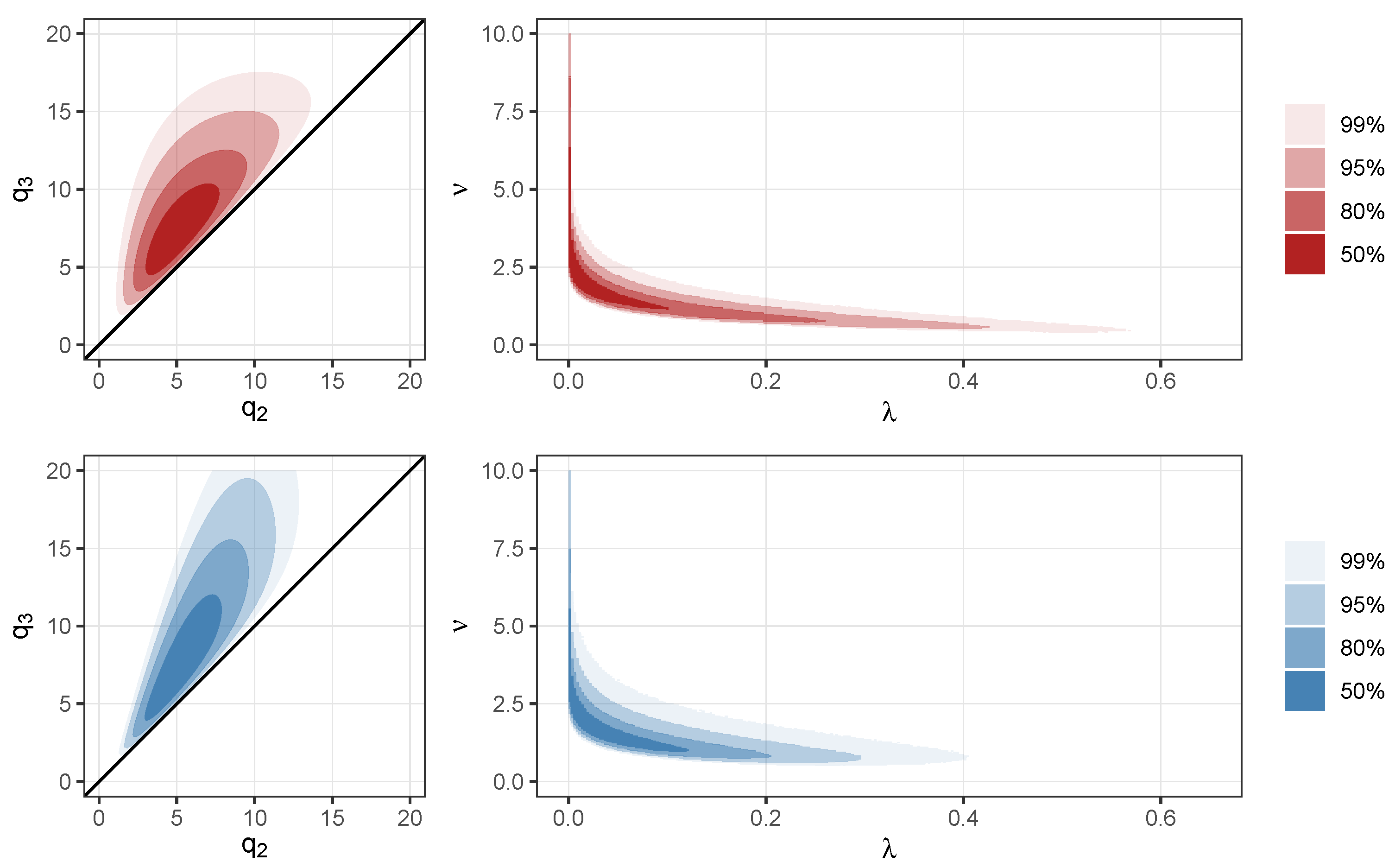
We start with the additive scheme. The response to is 2 months. This gives the most likely amount of additional time for half of the 50 hypothetical patients to experience an event. Hence, it is taken to be the mode of the gamma prior on w. The response to , 4 months, is the most optimistic amount of additional time needed for twenty-five of the fifty patients to experience an event. This value is taken to be the 75th percentile for the gamma prior on w. Setting the mode equal to 2 and the 75th percentile equal to 4 yields and . Under the additive scheme, the prior on is given by (9). The top row of Figure 1 plots the density of the joint prior distribution on the median and 75th percentile survival times, and the density of the induced joint prior distribution on the Weibull parameters and , respectively.
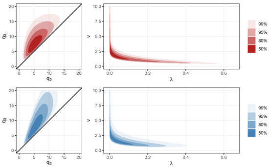
Figure 1.
Highest density region (HDR) plots of the elicited (left) and induced (right) joint priors when using the additive (top) and multiplicative (bottom) schemes. The legends communicate the probabilities associated with the HDRs [15].
Continuing this example, we use the multiplicative scheme to determine the prior on w. Once again, the answer to is the most likely amount for the additional time needed for half of the 50 patients to experience an event. Rather than taking the mode to be two months, we determine the percent increase in time between the 75th percentile and the median. This gives us , so a 40% increase in time. This percentage is the mode for the gamma prior on w. The response to gives the most optimistic time in addition to the median for 75 of the 100 patients to experience an event. Once again, we calculate the percent increase in time between the most optimistic 75th percentile and the median. This gives us , so an 80% increase in time between the median and the most optimistic 75th percentile. This percentage then makes up the 75th percentile for the gamma prior on w. Setting the mode equal to 40 and the 75th percentile equal to 80, we determine that and are equal to 2.90 and 0.05, respectively. The prior on is then determined by (10). The bottom row of Figure 1 plots the density of the joint prior distribution on the median and 75th percentile survival times, and the density of the induced joint prior distribution on the Weibull parameters and , respectively.
Focusing on the plots in the left column with the elicited times, we see that the prior using the multiplicative scheme has less variability for the lower values and increases in variability as times increase. Compared to the multiplicative scheme, the additive scheme has more variability for the lower values and less variability for . Now, focusing on the plots on the right, it is interesting that, regardless of the scheme used, the shape parameters of the gamma priors seem to have a similar spread, while the rate parameters tend to be much smaller for the multiplicative scheme. This is likely due to the fact that both schemes are anchored around the response for the most likely value for the median. In the additive scheme, we think of the responses to the last two questions as an addition to this most likely median time, while in the multiplicative scheme, we think of it as a percent increase from the most likely median time. Despite how the last two responses are incorporated into the elicitation, whether additively or multiplicatively, they are scaled versions of each other, which could account for the similarities in the shape parameter. Due to the similarities in the two schemes, we focus on the additive scheme going forward but consider the multiplicative scheme perhaps more intuitively appealing for a general application.
3. Results
A two-part simulation study was conducted to assess the performance of the additive scheme of the elicitation method. The first part of the simulation study investigated the accuracy and variability of each elicitation scheme in order to understand their sensitivity to expert misspecification. The second part of the simulation study investigated how the elicited priors compared in performance to a relatively non-informative prior.
3.1. Comparison of Elicited and Latent Priors
Assuming the Weibull is a suitable survival-time distribution, we seek a member of the Weibull family that aligns with an expert’s beliefs. We refer to this as the “latent prior” and its parameters as the “latent parameters”. Of course, in practice, the latent prior and its parameters are unknown. The first part of the simulation study is designed to investigate the priors that result when the parameters inferred from the elicited information differ from the latent parameters.
Since we cannot know the true parameters in practice, we proceeded as follows. For a given pair , we generated survival times as if they were elicited from well-informed experts. Specifically, we generated “elicited values” from a thousand hypothetical experts to evaluate how accurately our method estimates the latent values of and . We did this for different latent pairs , representing a variety of potential belief distributions, which are described below.
To ensure that the expert’s specifications aligned with the latent prior, we sampled the times-to-event for one hundred hypothetical patients from a Weibull distribution with the assumed latent parameters . For each hypothetical expert, the following steps were taken:
- The median of these one hundred survival times was taken as the response to .
- An additional time was added to the median, and this was taken as the response to . The amount added determined the informativeness of the hypothetical expert.
- The sample 75th percentile was computed, and the difference between this value and the median was taken as the response to .
- The response to was taken as the sum of the difference between the median and 75th percentile, and the second assigned additional time. Once again, this additional time was used to represent the informativeness of the hypothetical expert.
- Gamma priors for the median and additional time were constructed using the additive scheme and (4).
- Samples of ten thousand each for the median and 75th percentile survival times were drawn from their respective priors and transformed to obtain the priors for the shape and rate parameters of the Weibull distribution.
These samples were then used to construct the priors for and .
A range of latent shape and rate parameters was investigated via simulation. We took throughout, assuming the existence of prior modes at the cost of assuming increasing failure rates. Specifically, the shape parameter ranged from 1.05 to 1.25, and the rate parameter ranged from 0.25 to 0.45. Increasing increased the concentration of the Weibull density, making it more symmetric and peaked, thereby reducing variability. Similarly, increasing shifted more probability mass toward the origin, thereby further decreasing variability. Thus, increasing both and should result in a Weibull prior with less variability and an increasingly peaked shape, concentrated around the mode for .
One thousand iterations were run for each combination of shape and rate parameters. Another variable regarding the precision of the expert’s elicitation, or informativeness of the elicitation, was investigated by varying the amount of time added to the sample statistics. For the first design point, considered informative, the amount of time added to the median was one time unit, and the additional time added to the difference was two units. For the second design point, considered less informative, the times added to the median and difference were six time units and nine time units, respectively. By increasing the amount of time added to the modes of each distribution, we increased the variability of the elicited gamma priors. Thus, we had three variables under investigation: the shape parameter, the rate parameter, and the expert’s uncertainty. For each elicitation scheme, this resulted in investigating fifty design points arising from each combination of a rate parameter, a shape parameter, and the expert’s level of uncertainty.
Figure 2 displays the average marginal prior intervals for the parameters when the additive elicitation scheme was used. Each of the plots displays the average 95% intervals for the marginal priors elicited for and , where the vertical line denotes the true value of and , and the points represent the median for each parameter. As the values of and increase, the 95% intervals become wider regardless of how much additional time was added to obtain the optimistic times. As expected, the more time we added to obtain the optimistic times, the more variability was present in the marginal priors.
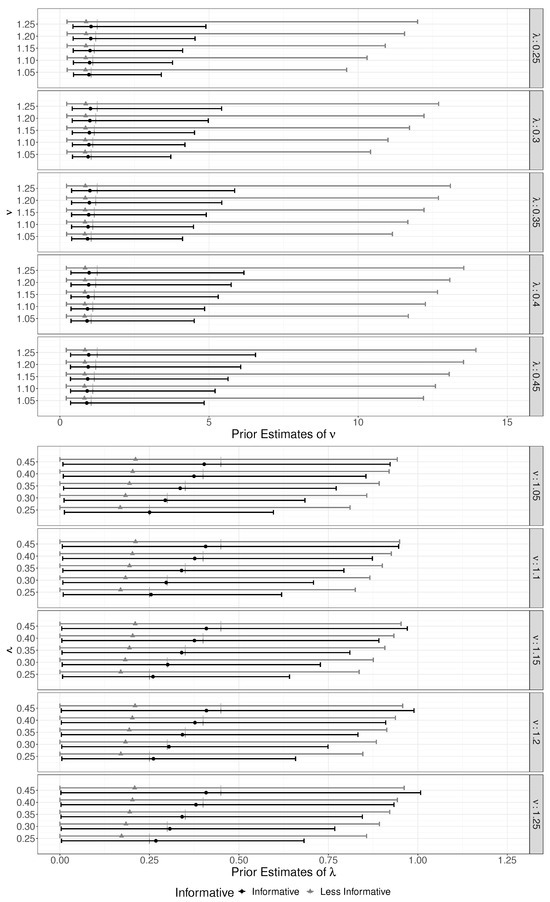
Figure 2.
The average 95% intervals for the elicited marginal priors for (top) and (bottom) using the additive scheme. The two different colors represent the levels of informativeness, specified based on the precision of the elicitation.
3.2. Posterior Consequences of Using Elicited vs. Non-Informative Priors
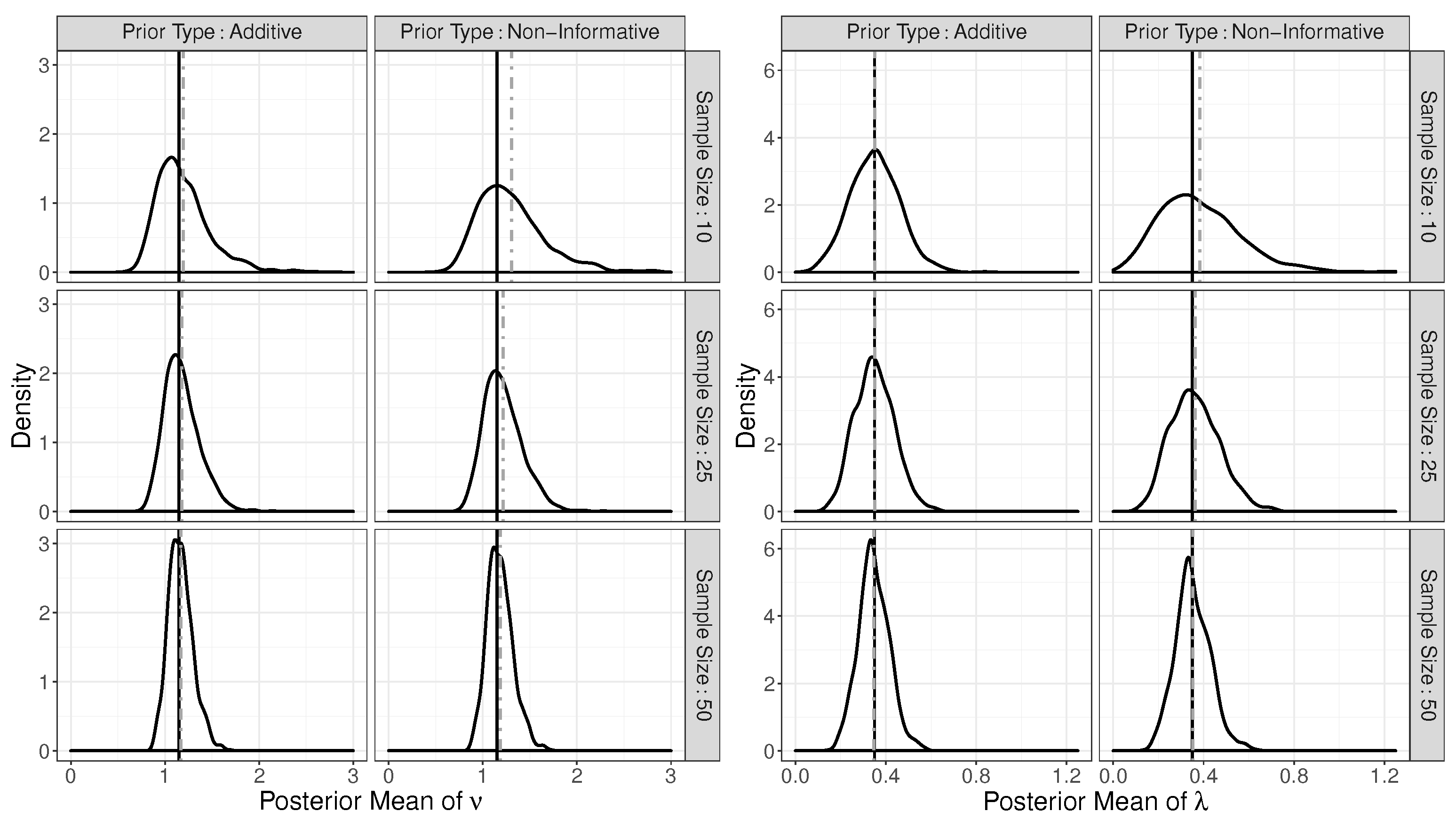
The second part of the simulation study compared the marginal posteriors that resulted when using an elicited prior to those resulting from a relatively non-informative prior. Non-informative priors express a lack of prior belief about the parameter being estimated and are often represented via a flat distribution. Informative priors are the opposite and are used when we have some prior belief to inform the parameters being estimated. In this simulation study, the two variables that were investigated were the type of prior distribution that was used—whether it was constructed via the elicitation scheme or was a relatively non-informative prior—and the sample size of the data used to form the likelihood function. The size of the data varied to investigate how the marginal posteriors from each prior were affected as the sample size increased. The sample sizes investigated in this simulation study were 10, 25, and 50. A sample size of ten is usually the target in clinical trials for rare diseases or pediatric clinical trials. A total of six design points were investigated in this simulation, resulting from combining the two types of prior distributions and the three sample sizes. The latent Weibull distribution in this simulation had a shape of 1.15 and a rate of 0.35 and was motivated by the results of an actual elicitation involving six experts regarding an oncology trial.
One thousand iterations were run for each value of the sample size investigated. For each iteration, the informative priors were constructed using the same methodology as in Section 3.1, where the time added to the median was one month and the time added to the additional time was two months. The data used in each iteration of the simulation was a sample of an assigned size from the latent survival distribution with and . For each iteration, a Bayesian model was fitted using the sampled data and each of the two types of priors, with the elicited priors using the additive scheme and relatively non-informative Gamma priors. For this simulation, both and had Gamma() priors.
Table 1 summarizes the marginal posteriors for and for each scenario. As the sample size increased, the width of the 95% credible intervals decreased, as expected, regardless of the prior used. When the priors were elicited using the additive scheme, the posterior means of were closer to the latent value of 1.15 compared to the posterior means when using the relatively non-informative priors. For a sample size of ten, the 95% credible intervals of the marginal posteriors that resulted from using a relatively non-informative prior were wider than the intervals obtained from using either of the elicited priors, again as expected.

Table 1.
Summary of marginal posterior distributions for and using two different types of priors and different sample sizes for the data.
Figure 3 displays the densities of the posterior means for and for each sample size and type of prior. The solid vertical line represents the latent value of each parameter, and the dashed line represents the average of the posterior means for each scenario. Not surprisingly, when the sample size was very small, the use of a relatively non-informative prior resulted in wide marginal posterior densities with noticeably biased estimates of the true values. At a sample size of 25, the differences in the variability in the posterior densities using different types of priors were less noticeable, and at a sample size of 50, the variability was almost the same.
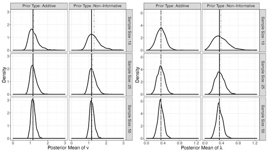
Figure 3.
Density plots of marginal posterior means for (left) and (right) across varying sample sizes, using an elicited prior (first column) and a non-informative prior (second column).
3.3. Application
The elicitation method using the additive scheme was applied to a pediatric clinical trial for a rare form of cancer. Elicitations were obtained from multiple experts. The aim of this process was to obtain probability distributions that represent current knowledge and uncertainty about the time points of interest. The endpoint of interest in this elicitation was progression-free survival (PFS). In the Bayesian model, we assumed that the time to PFS had a Weibull distribution. The expert opinion obtained via prior elicitation served to augment the small control arms in planned clinical trials.
Information was elicited from six experts in the field. Each elicitation was performed separately during an approximately hour-long video conference. There were two facilitators for the elicitation, as well as two statisticians collecting data and giving statistical feedback. The process began with the first facilitator giving a brief introduction to the research problem, the elicitation process, and the goal of the elicitation. The four questions that were asked of each expert were as follows:
- Imagine you have 100 patients; how many months would you expect it to take for half of those patients to have documented progressive disease?
- For those same 100 patients, what is the most optimistic guess for that time that someone could give?
- Of the remaining 50 patients, how many more months would you expect it to take for half of these 50 patients to have a PFS event?
- For those same remaining 50 patients, what is the most optimistic guess for that time that someone could give?
After introducing the questions to the experts, an example elicitation was performed using graphics to further assist the expert in understanding how the elicitation process would be conducted. After the expert answered the first two questions, the elicited prior for the median PFS was shown to the expert, along with a visual of the related consequences consistent with those beliefs. This feedback afforded a check on the adequacy of the elicited distribution. If the expert agreed with the distribution, the facilitator proceeded to the last two questions. If the expert did not agree with the elicited distribution, appropriate changes were made until the elicited distribution best conveyed the expert’s knowledge. After the expert’s knowledge about the additional time was elicited, the induced prior distribution for the 75th percentile PFS times, which, as shown in (9), is a sum of the median PFS and the additional PFS, was shown to the expert rather than the elicited distribution for the additional time. Once again, an adequacy check was performed until the elicited distribution best represented the expert’s knowledge. An overall validation was then conducted by showing the expert visualizations (e.g., histograms) based on synthetic samples drawn from the prior predictive distribution [6]. If the expert deemed these to be reasonable, the prior was considered to be confirmed.
The elicitation was performed for various control and backbone regimens; however, this process is illustrated only for one of those arms. The information elicited, in months, from the experts for one of the control arms is given in Table 2. There is some variability among the responses given by the experts, especially for the optimistic times.
Table 2.
Elicited values, in months, for a control arm from multiple experts.
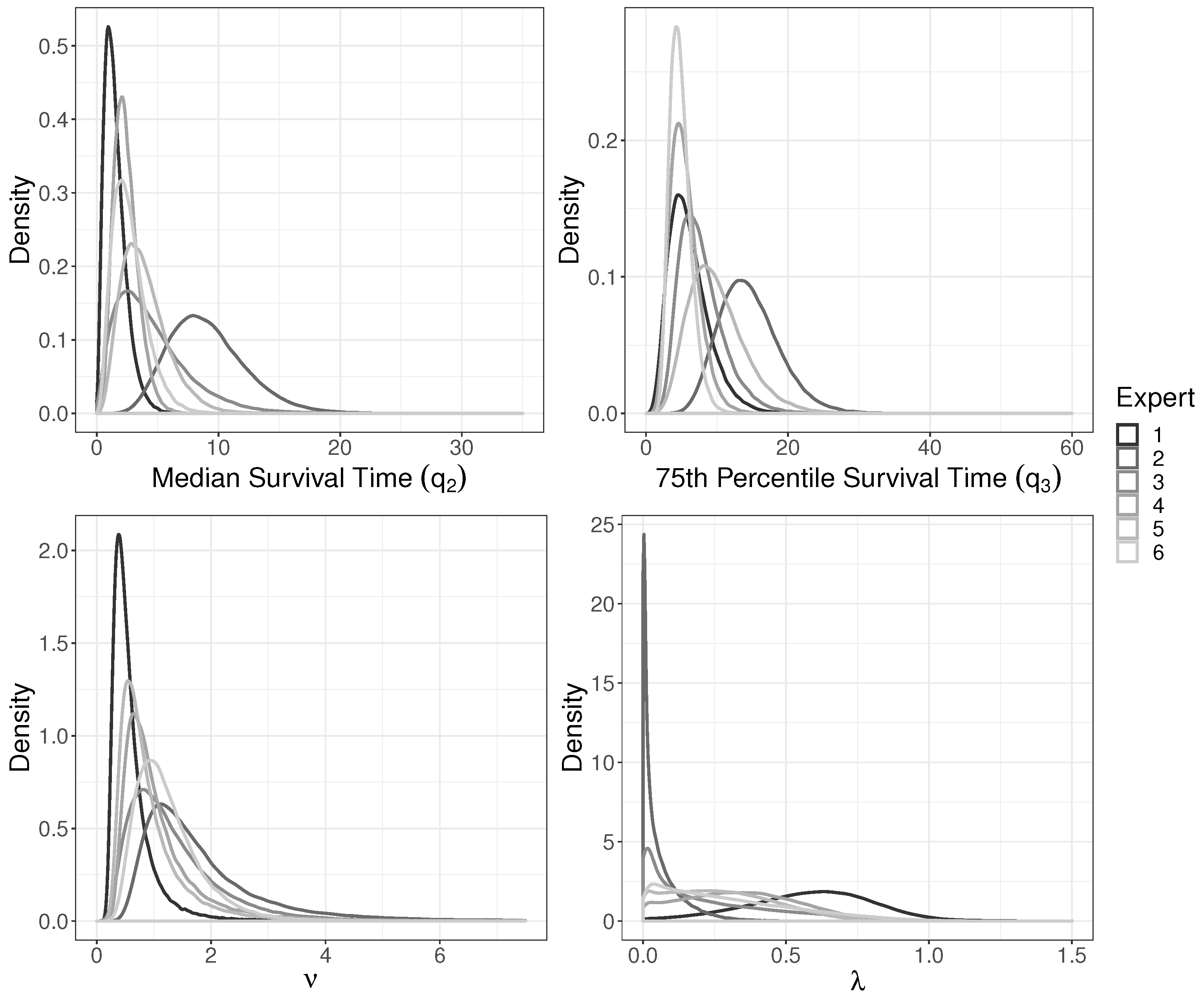
Using the times elicited in Table 2, priors were constructed for the median and 75th percentile for the time to PFS. These times were then transformed to obtain the priors on the Weibull parameters and , as described in Section 2. Figure 4 displays each of the prior distributions that were elicited. The variability in responses among the experts can be seen in the priors for the median and upper-quartile PFS times. After transforming these times to obtain the parameters, less variability can be seen among the experts for the shape parameter, but the distributions of vary due to the differences in the expert elicitations. For example, the second expert’s knowledge is very different from that of the other experts, which can be seen in each of the elicited distributions in Figure 4. Rather than using each distribution separately, the elicited priors could be synthesized into a single elicitation using methods such as logarithmic pooling or equally weighted mixtures.
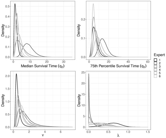
Figure 4.
Priors elicited for each of the six experts on the median (top left) and 75th percentile times (top right). The additive elicitation scheme was used to induce the marginal priors on (bottom left) and (bottom right).
4. Discussion
The Weibull distribution is widely used to model time-to-event data. For Bayesian models with a Weibull likelihood, the specification of a joint prior is required for the shape and rate parameters. Each of these is typically modeled with a distribution from a two-parameter family, for a total of four independent hyperparameters. The prior distributions in these families vary in their levels of informativeness, so some priors imply that very little is known about the parameters, in which case data will have a significant influence on the posterior belief (which might still be very uncertain), whereas others communicate moderate or strong prior beliefs in the values, counterbalancing the data and guiding or potentially even forcing the analysis to a certain conclusion, so care must be taken when specifying priors. If sufficient data is collected for a clinical trial, a relatively non-informative prior can be used; however, this is rarely the case for most clinical trials investigating rare diseases or diseases in children. In such cases, an informative prior distribution is often desirable. Such a prior can be constructed using historical data (if available) or expert opinion. Prior elicitation is a principled strategy for converting expert opinion into these prior distributions, represented here by the four hyperparameters.
In this paper, we presented a new method for eliciting priors for the Weibull parameters. The proposed method can elicit priors using either an additive scheme or a multiplicative scheme that induces a four-parameter prior family on the bivariate parameter space of the Weibull distribution. The proposed methods work by eliciting survival times that can then be inverted to induce prior distributions on the parameters indexing the Weibull family. These survival times are more easily quantified by experts since these values are on an observable scale.
We also presented a simulation study, which showed that the induced priors are reasonably sensitive to changes in an expert’s uncertainty. The more uncertainty present in the expert’s responses, the more uncertainty is present in the induced priors. In both parts of the simulation study, we saw that the multiplicative scheme resulted in slightly more informative priors than the additive scheme.
In addition, we illustrated a real-world scenario where the method was used to elicit priors for a pediatric clinical trial in which rare forms of cancer were being investigated. Information was elicited from six experts who differed considerably in their responses (pooling or resolving different experts’ beliefs was not discussed). The additive scheme was used to elicit priors on the median and 75th percentile PFS times. These priors were then transformed to induce priors on and .
In conclusion, the proposed elicitation method shows promising results when an informative joint prior is needed for the Weibull distribution. One of the key advantages of our method is that we elicit information on an observable scale rather than directly on the prior parameters, which are not otherwise easily interpretable. This advantage is necessary when experts, such as physicians, are not familiar with the Weibull distribution. From the application, we can see that small changes in the elicited values can result in different distributions. Further work needs to be carried out to investigate this elicitation method, including investigating how sensitive the resulting priors are to changes in elicited values and quantifying the informativeness of these elicited priors.
Author Contributions
Conceptualization, P.P., J.D.S., D.K., J.W.S.J., Z.M.T. and M.S.; methodology: P.P., J.D.S., D.K. and J.W.S.J.; investigation, P.P.; formal analysis, P.P.; writing—original draft, P.P., J.D.S., D.K. and J.W.S.J.; writing—review and editing, P.P., J.D.S., D.K., J.W.S.J., Z.M.T. and M.S.; visualization, P.P. and D.K. All authors have read and agreed to the published version of the manuscript.
Funding
This research received no external funding.
Institutional Review Board Statement
Not applicable.
Informed Consent Statement
Not applicable.
Data Availability Statement
The original contributions presented in this study are included in the article. Further inquiries can be directed to the corresponding author.
Conflicts of Interest
Purvi Prajapati, Zachary M. Thomas, and Michael Sonksen are employees and minor shareholder of Eli Lilly and Company.
References
- Brard, C.; Teuff, G.L.; Le Deley, M.; Hampson, L.V. Bayesian survival analysis in clincial trials: What methods are used in practice? Clin. Trials 2017, 14, 78–87. [Google Scholar] [CrossRef]
- Campodónico, S.; Singpurwalla, N.D. Expert Opinion in Reliability; George Washington University Institute for Reliability and Risk Assessment: Washington, DC, USA, 1993; pp. 1–18. [Google Scholar]
- Hamspon, L.V.; Whitehead, J.; Eleftheriou, D.; Tudur-Smith, C.; Jones, R.; Jayne, D.; Hickey, H.; Beresford, M.W.; Bracaglia, C.; Caldas, A.; et al. Elicitation of Expert Prior Opinion: Application to the MYPAN Trial in Childhood Polyarteritis Nodosa. PLoS ONE 2015, 10, e0120981. [Google Scholar]
- O’Hagan, A.; Buck, C.E.; Daneshkhah, A.; Eiser, J.R.; Garthwaite, P.H.; Jenkinson, D.J.; Oakley, J.E.; Rakow, T. Uncertain Judgements: Eliciting Experts’ Probabilities; John Wiley & Son, Ltd.: Hoboken, NJ, USA, 2006. [Google Scholar]
- Montague, T.H.; Price, K.L.; Seaman, J.W., Jr. The Practice of Prior Elicitation. In Bayesian Applications in Pharmaceutical Development; Natanegara, F., Lakshminarayanan, M., Eds.; CRC Press: Boca Raton, FL, USA, 2006; pp. 61–92. [Google Scholar]
- Garthwaite, P.H.; Kadane, J.B.; O’Hagan, A. Statistical Methods for Eliciting Probability Distributions. J. Am. Stat. Assoc. 2005, 100, 680–701. [Google Scholar] [CrossRef]
- Oakley, J.E.; O’Hagan, A. SHELF: The Sheffield Elicitation Framework (Version 4.0). Available online: http://tonyohagan.co.uk/shelf (accessed on 1 November 2024).
- Oakley, J.E.; Ren, S.; Forsyth, J.E.; Gosling, J.P.; Wilson, K.; Latimer, N.; Rutherford, M.J.; Uttley, L.; Fotheringham, J. NICE DSU Technical Support Document 26: Expert Elicitation for Long-Term Survival Outcomes. NICE Decision Support Unit Technical Support Document Series. 2025, pp. 1–114. Available online: https://www.nicedsu.org.uk (accessed on 27 April 2025).
- Singpurwalla, N.D. An Interactive PC-Based Procedure for Reliability Assessment Incorporating Expert Opinion and Survival Data. J. Am. Stat. Assoc. 1988, 83, 43–51. [Google Scholar] [CrossRef]
- Gutiérrez-Pulido, H.; Aguirre-Torres, V.; Christen, J.A. A Practical Method for Obtaining Prior Distributions in Reliability. IEEE Trans. Reliab. 2005, 54, 262–269. [Google Scholar] [CrossRef]
- Bousquet, N. Elicitation of Weibull Priors. arXiv 2010, arXiv:1007.4740. [Google Scholar]
- Blair, S. Contributions to the Theory and Practice of Prior Elicitation in Biopharmaceutical Research. Ph.D. Thesis, Baylor University, Waco, TX, USA, May 2017. [Google Scholar]
- Ren, S.; Oakley, J.E. Assurance calculations for planning clinical trials with time-to-event outcomes. Stat. Med. 2014, 33, 31–45. [Google Scholar] [CrossRef] [PubMed]
- O’Hagan, A. Eliciting Expert Beliefs in Substantial Practical Applications. J. R. Stat. Soc. Ser. (Statstician) 1998, 47, 21–35. [Google Scholar]
- Otto, J.; Kahle, D. ggdensity: Improved Bivariate Density Visualization in R. R J. 2023, 15, 220–236. [Google Scholar] [CrossRef]

Disclaimer/Publisher’s Note: The statements, opinions and data contained in all publications are solely those of the individual author(s) and contributor(s) and not of MDPI and/or the editor(s). MDPI and/or the editor(s) disclaim responsibility for any injury to people or property resulting from any ideas, methods, instructions or products referred to in the content. |
© 2025 by the authors. Licensee MDPI, Basel, Switzerland. This article is an open access article distributed under the terms and conditions of the Creative Commons Attribution (CC BY) license (https://creativecommons.org/licenses/by/4.0/).