Distance-Based Relevance Function for Imbalanced Regression

Abstract

Imbalanced regression poses a significant challenge in real-world prediction tasks, where rare target values are prone to overfitting during model training. To address this, prior research has employed relevance functions to quantify the rarity of target instances. However, existing functions often struggle to capture the rarity across diverse target distributions. In this study, we introduce a novel Distance-based Relevance Function (DRF) that quantifies the rarity based on the distance between target values, enabling a more accurate and distribution-agnostic assessment of rare data. This general approach allows imbalanced regression techniques to be effectively applied to a broader range of distributions, including bimodal cases. We evaluate the proposed DRF using Mean Squared Error (MSE), relevance-weighted Mean Absolute Error ($\mathrm{MAE}\varphi$), and Symmetric Mean Absolute Percentage Error (SMAPE). Empirical studies on synthetic datasets and 18 real-world datasets demonstrate that DRF tends to improve the performance across various machine learning models, including support vector regression, neural networks, XGBoost, and random forests. These findings suggest that DRF offers a promising direction for rare target detection and broadens the applicability of imbalanced regression methods.

1. Introduction

In imbalanced classification—where the minority class is significantly underrepresented—standard learning algorithms often overfit rare examples. To address this, both data-level and algorithm-level solutions have been proposed. A key data-level approach is SMOTE [1], which generates synthetic minority samples via linear interpolation. Combined with majority undersampling, this improves rare-class sensitivity without sacrificing the overall accuracy. In parallel, statistical corrections for rare event bias have been proposed in the modeling stage. For example, King and Zeng [2] highlight how standard logistic regression tends to underestimate the probability of rare events and offer bias correction methods and efficient sampling strategies to improve the predictive accuracy in imbalanced settings.

However, research on imbalanced regression—where the target is continuous—remains limited. Unlike classification, there are no discrete labels to guide resampling. This makes it challenging to define principled rules for identifying which regions of the target distribution warrant augmentation or pruning, rendering resampling in regression inherently more complex.

To address the scarcity of rare targets, prior work introduced relevance functions that assign a normalized rarity score in [0,1] to each continuous target [3]. This stems from the insight that extreme outcomes often hold disproportionate importance in domains like customer analytics, finance, and meteorology. A common approach uses box-plot statistics, labeling values beyond interquartile “whiskers” as highly relevant. However, this tail-focused assumption limits applicability in cases where rare events arise in central or multimodal regions of the distribution.

To move beyond tail-based relevance, we propose the Distance-based Relevance Function (DRF), which quantifies rarity by measuring each target’s proximity to others. DRF highlights sparse regions—whether in the tails, between modes, or elsewhere—without relying on distributional assumptions. This makes it broadly applicable across unimodal, bimodal, and complex distributions. We validate DRF on simulated and 18 real-world datasets using SVR, neural networks, XGBoost, and random forests, evaluating the performance with task-appropriate metrics.

The remainder of this paper is organized as follows. Section 2 reviews prior research on imbalanced regression and introduces the evaluation metrics used throughout the study. Section 3 presents the proposed methodology, including the formulation of DRF. Section 4 provides experimental results and analysis on both simulated and real-world datasets. Finally, Section 5 concludes the paper with a summary of the findings and directions for future work.

2. Preliminaries

2.1. Previous Research

In imbalanced regression, a relevance function maps continuous target values to the [0, 1] range, assigning higher scores to rare observations [3]. This extends the idea of class imbalance to regression, where rare and normal targets parallel the minority and majority classes in classification. The relevance function guides resampling by highlighting critical regions of the target space where improved predictive accuracy is most needed.

The earliest relevance function, proposed by Torgo et al. [3], uses box-plot statistics—median, interquartile range, and whisker endpoints—to define sigmoid curves that assign a relevance of 0 at the median and 1 at the extremes. This tail-focused approach underpins methods such as SMOTER [4], which over-samples high-relevance observations via k-nearest-neighbor interpolation, and SMOGN [5], which further improves the sample quality by injecting Gaussian noise when the nearest neighbors are too distant. However, both methods assume that rare observations reside at the extremes, making them less effective for non-extreme or multimodal distributions.

To address this limitation, kernel-density-based relevance functions have been proposed. For instance, DenseWeight [6] assigns relevance as the inverse of the estimated probability density function, while KSMOTER [7] builds similar functions using kernel density estimation and analyzes the impact of bandwidth selection. These approaches make no assumptions about the location of rare values, allowing for broader applicability. However, they depend heavily on kernel choices and shape parameters, making them sensitive to data quality and hyperparameter tuning.

Recent advances in imbalanced regression have introduced more flexible methods for handling rare target values. Geometric SMOTE [8] generates synthetic examples within localized geometric regions, while deep learning techniques like Label Distribution Smoothing (LDS) and Feature Distribution Smoothing (FDS) improve prediction by smoothing target and feature distributions during training [9]. Gonzalez-Abril et al. [10] extend this work by exploring preprocessing strategies such as fuzzy logic and meta-learning, and Branco et al. [11] propose relevance-aware metrics for evaluating rare-target performance in multi-target regression. Despite these advances, many methods rely on user-defined parameters or complex estimation procedures, which can reduce the robustness. This motivates the development of adaptive, distribution-agnostic approaches to relevance estimation and resampling.

To address these shortcomings, we introduce DRF, a fully parameter-free function that measures rarity exclusively via pairwise distances among target values. Our approach is inherently robust to noise and kernel choice, and it applies to any target distribution—even those with non-extreme or multimodal rare regions.

2.2. Performance Measures

Choosing appropriate performance metrics is crucial for imbalanced regression, where the focus is on accurately predicting rare target values. Unlike classification’s binary labels, regression outputs are continuous, so correctness must be defined by an error tolerance. Some approaches treat predictions within a fixed error bound as correct and compute an F1-style score [12], but the choice of that tolerance is arbitrary and can dramatically alter the outcome. Consequently, such threshold-based metrics may be unreliable for evaluating imbalanced regression.

We assess the overall predictive performance using the Mean Squared Error (MSE) and highlight the accuracy on rare targets with a relevance-weighted Mean Absolute Error (MAE$\varphi$), which weights each error by the corresponding data point’s rarity [13]. To ensure scale invariance, we also report Symmetric Mean Absolute Percentage Error (SMAPE), which measures percentage deviation without the upward bias of standard MAPE. The corresponding formulas are given below:

$$\begin{array}{c}\hfill \begin{array}{c}\mathrm{MSE}={\displaystyle \frac{1}{N}}{\displaystyle \sum _{i=1}^N}{(y_i-{\widehat{y}}_i)}^2\end{array}\end{array}$$

(1)

$$\begin{array}{c}\hfill \begin{array}{c}\mathrm{MAE}\varphi =\sqrt{{\displaystyle \frac{1}{N}}{\displaystyle \sum _{i=1}^N}\varphi \left(y_i\right)\times |y_i-{\widehat{y}}_i|}\end{array}\end{array}$$

(2)

$$\begin{array}{c}\hfill \begin{array}{c}\mathrm{SMAPE}={\displaystyle \frac{100\%}{N}}{\displaystyle \sum _{i=1}^N}{\displaystyle \frac{|y_i-{\widehat{y}}_i|}{\left(\right|y_i|+|{\widehat{y}}_i\left|\right)/2}},\end{array}\end{array}$$

(3)

where, N is the number of observations, $y_i$ the true value, and ${\widehat{y}}_i$ the prediction of the ith observation.

3. Proposed Method

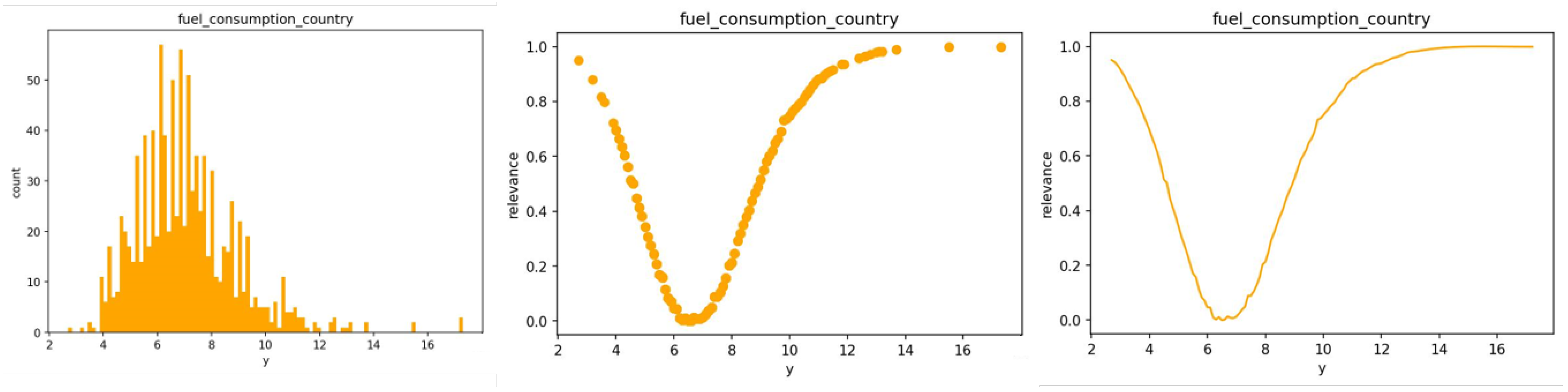
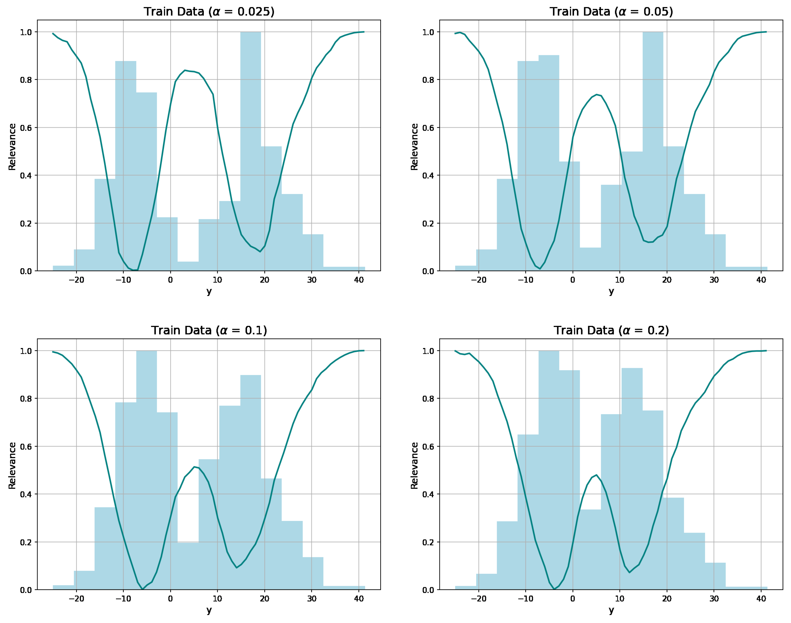
3.1. Distance-Based Relevance Function

We propose the Distance-based Relevance Function (DRF) that quantifies rarity solely from the one-dimensional distribution of target values. Let $\{y_1,\dots ,y_n\}$ be our observed targets (after standardization). For each observation y, we first compute a raw score that reflects both the number of neighbors and their proximity:

$$s\left(y\right)=\sum _{i=1}^n{\displaystyle \frac{\mathbb{I}\left(\right|y-y_i|<D)}{|y-y_i|+\delta }},$$

where $D=1$ (one standard deviation) defines the search radius to ignore distant points, and $\delta =1$ is a small stabilization constant preventing division-by-zero when $|y-y_i|\approx 0$.

Because $s\left(y\right)$ grows with local density, rarer (more isolated) points produce smaller scores. We therefore invert and normalize these scores to yield relevance values in $[0,1]$:

$${\varphi }_D\left(y\right)={\displaystyle \frac{{max}_{j}s\left(y_j\right)-s\left(y\right)}{{max}_{j}s\left(y_j\right)-{min}_{j}s\left(y_j\right)}}.$$

Finally, we apply a smooth cubic Hermite interpolation to the discrete pairs $\left\{(y,{\varphi }_D\left(y\right))\right\}$, producing a continuous relevance function over the entire target range.

Figure 1 illustrates how DRF adapts to a skewed histogram of targets without any reliance on box-plot extremes. For completeness, the pseudocode for computing DRF is included as Algorithm A1 in Appendix A.

3.2. DRF-SMOGN

We integrate DRF into the SMOGN framework to form DRF-SMOGN. First, we compute the distance-based relevance score ${\varphi }_D\left(y\right)$ for each instance and partition the data into rare and normal bins via a relevance threshold $t_R$. We then apply random under-sampling of the normal bin at u% and random over-sampling of the rare bin at o%.

For each rare bin B, we randomly sample seed instances and, for each seed x, identify its k nearest neighbors using the Heterogeneous Euclidean–Overlap Metric (HEOM) [14], which applies Euclidean distance to normalized numerical features and overlap distance to nominal features.

We compute a safety threshold:

$$\mathrm{maxD}=\frac{1}{2}\mathrm{median}\left(\mathrm{distances}(x,B)\right).$$

To generate each synthetic instance, we pick one neighbor $x_{\mathrm{neigh}}$. If $\mathrm{dist}(x,x_{\mathrm{neigh}})<\mathrm{maxD}$, we perform SMOTER-style linear interpolation; otherwise, we add Gaussian noise with standard deviation $min(\mathrm{maxD},0.02)$ to x. Over-sampled predictors are paired with target values computed as a distance-weighted average of the two originals.

For clarity, Algorithm A2 in Appendix B provides a summary of the full DRF-SMOGN procedure, covering the steps from relevance-based binning to the conditional use of SMOTER or noise generation, followed by the final target assignment.

The DRF-SMOGN pipeline makes no distributional assumptions or user-tuned shape parameters, yet retains SMOGN’s adaptive interpolation vs. noise balance—now driven by a fully parameter-free relevance metric. Because DRF imposes no constraints on the placement of rare observations, it applies seamlessly to any target distribution—including bimodal cases—and can even generate multiple rare or normal bins, marking a significant advance over prior relevance functions.

4. Experimental Study

4.1. Data Description

4.1.1. Simulation Data

Simulation datasets were generated to evaluate DRF-SMOGN on bimodal target distributions, reflecting scenarios where rare observations may appear anywhere in the target space.

Each simulation dataset consists of a training set, intentionally made bimodal by removing values near the median, and a test set that follows the original unimodal distribution (Figure 2). Both sets originate from the same nonlinear relationship involving six predictor variables. To induce bimodality, we define an interval around the median of the target values and delete each observation within this interval with probability

$$p\left(y\right)=1-exp\left(-\alpha \times |y-\mathrm{median}(Y\left)\right|\right),$$

where $\alpha$ is a rarity constant. As $\alpha$ decreases, the deletion probability near the median increases, removing more central observations and creating a more pronounced bimodal gap. This mechanism ensures that rare regions (away from the median) become denser relative to the center.

We report the average training and test set sizes over 100 replications for each rarity constant $\alpha$. The test set size is fixed at 300 samples across all settings. As $\alpha$ increases, fewer deletions occur near the median, resulting in larger training sets. Specifically, the average training sizes corresponding to $\alpha =0.025,0.050,0.100,$ and $0.200$ are 1161, 1350, 1663, and 2055, respectively.

Figure 3 shows both the histogram of each training set and the corresponding DRF relevance curve. As $\alpha$ increases, the gap around the median narrows and DRF smoothly captures the emerging dense and sparse regions, demonstrating its ability to adapt to varying rarity patterns.

4.1.2. Real Data

To evaluate DRF on real data, we selected 18 publicly available benchmark datasets, consistent with prior imbalanced-regression studies focusing on extreme-tail imbalance [4]. These datasets are available at https://www.dcc.fc.up.pt/~ltorgo/EPIA2013/.

Table 1. Characteristics of real datasets: sample size (N), predictor counts ($p_{\mathrm{total}}$), number of nominal ($p_{\mathrm{nom}}$) and numerical ($p_{\mathrm{num}}$) predictors, rare-observation count ($n_{\mathrm{Rare}}$), and rarity percentage (% Rare, ${\varphi }_D\left(y\right)\ge 0.8$).

Dataset	N	${\mathit{p}}_{\mathbf{total}}$	${\mathit{p}}_{\mathbf{nom}}$	${\mathit{p}}_{\mathbf{num}}$	${\mathit{n}}_{\mathbf{Rare}}$	% Rare
a1	198	11	3	8	46	23.2
a2	198	11	3	8	35	17.7
a3	198	11	3	8	34	17.2
a4	198	11	3	8	27	13.6
a5	198	11	3	8	30	15.2
a6	198	11	3	8	33	16.7
a7	198	11	3	8	27	13.6
abal	4177	8	1	7	679	16.3
accel	1732	15	3	12	137	7.9
avail	1802	16	7	9	217	12.0
bank	4499	9	0	9	662	14.7
bost	506	13	0	13	76	15.0
cpu	8192	13	0	13	755	9.2
dAil	7129	5	0	5	773	10.8
dElev	9517	6	0	6	990	10.4
fuel	1764	38	12	26	248	14.1
heat	7400	12	8	4	802	10.8
maxt	1802	33	13	20	129	7.2

summarizes each dataset’s characteristics: total sample size N, total number of predictors $p_{\mathrm{total}}$, counts of nominal ($p_{\mathrm{nom}}$) and numerical ($p_{\mathrm{num}}$) predictors, number of rare observations $n_{\mathrm{Rare}}$, and rarity percentage (% Rare), where rarity is defined by ${\varphi }_D\left(y\right)\ge 0.8$.

Although these real-world targets are unimodal, their skewness varies widely—some are heavily skewed, placing rare values only in one tail. Because DRF does not assume that rarity lies at the extremes, it naturally adapts to these different shapes.

4.2. Method

We present our DRF–SMOGN approach, which combines DRF with the SMOGN over-sampling procedure.

4.2.1. Relevance Threshold

DRF requires no extra hyperparameters beyond the relevance threshold $t_R$, a user-specified cutoff also used in prior works [3]. For our simulation studies, we set

$$t_R=\left\{\begin{array}{cc}0.6,\hfill & \alpha \in \{0.025,0.05\},\hfill \\ 0.4,\hfill & \alpha \in \{0.10,0.20\},\hfill \end{array}\right.$$

since higher $\alpha$ produces fewer central deletions and thus lower raw relevance scores. Across all 18 real-world datasets, we adopt a relevance threshold of $t_R=0.8$, in line with prior studies [5,6].

4.2.2. Sampling via SMOGN

Once each observation is assigned ${\varphi }_D\left(y\right)$, we partition the data into rare (${\varphi }_D\left(y\right)\ge t_R$) and normal (${\varphi }_D\left(y\right)<t_R$) bins. Normal bins undergo random under-sampling at rate $p_u$, while rare bins are over-sampled at rate $p_o$, exactly as in SMOGN [5]. Key SMOGN hyperparameters include the number of neighbors k and the Gaussian perturbation constant $\mathit{pert}$. To ensure fair comparison, we adopt the original SMOGN settings $k=5$ and $pert=0.02$. Other settings such as the over-sampling and under-sampling rates were kept the same as well.

4.2.3. Experimental Setup

We compare three sampling strategies—none (original data), SMOGN, and DRF–SMOGN—using four regressors:

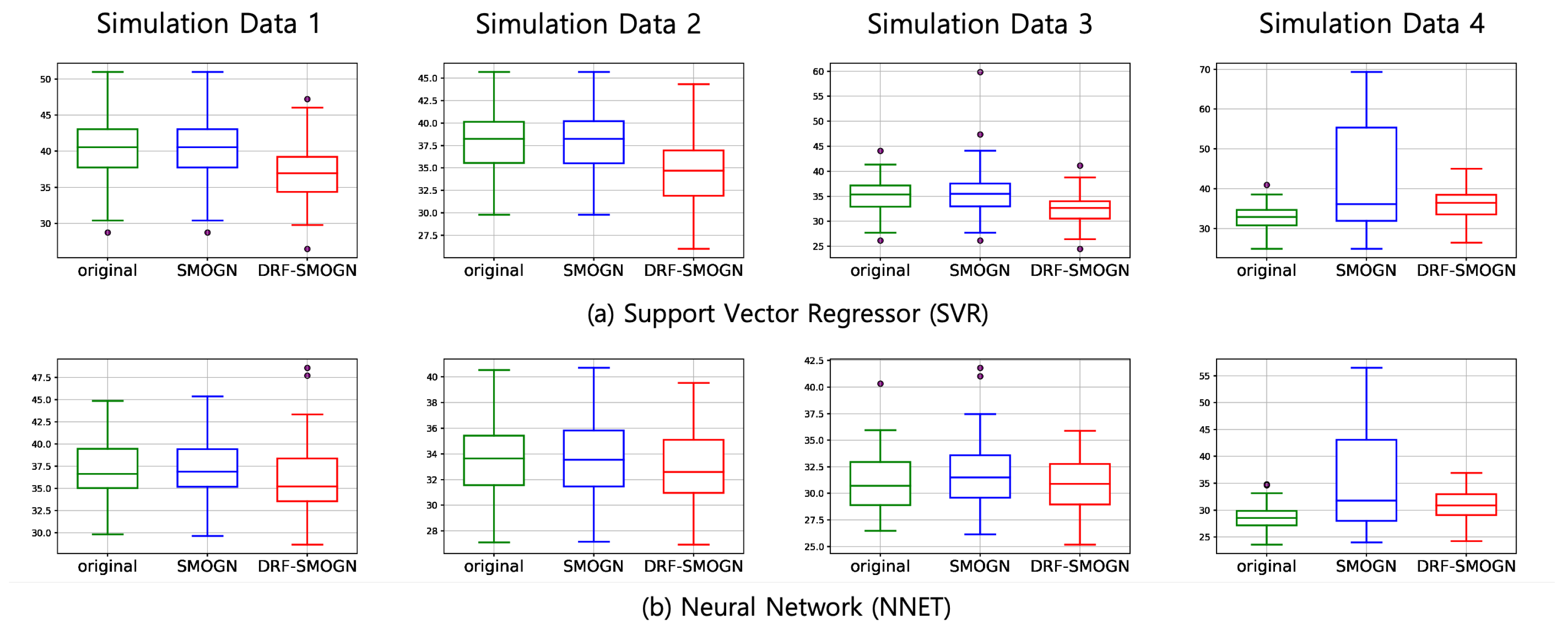
• Support Vector Regressor (SVR).
• Neural network (NNET).
• XGBoost Regressor (XGB).
• Random Forest Regressor (RF).

All models are tuned on the original (unsampled) data via grid search; the parameter ranges are shown in

Table 2. Regressor hyperparameter grid for SVR, NNET, XGB, and RF.

Learner	Parameter Variants
SVR	$C\in \{10,150,300\},\gamma \in \{0.01,0.001\}$
NNET	hidden_layer_sizes $\in \{1,5,10,50\}$, activation $\in \left\{\mathrm{identity},\mathrm{logistic},\tan \mathrm{h},\mathrm{relu}\right\}$,
	solver $\in \left\{\mathrm{lbfgs},\mathrm{sgd},\mathrm{adam}\right\}$, alpha $\in \{5\times {10}^{-5},5\times {10}^{-4},5\times {10}^{-3}\}$
XGB	learning_rate $\in \{0.1,0.5\}$, n_estimators $\in \{500,1000\}$, max_depth $\in \{3,5,7\}$
RF	n_estimators $\in \{100,200,500,700,1500\}$, max_depth $\in \{3,5,7\}$

. Simulation datasets are replicated 100 times, and each real-world dataset is assessed over 100 random train–test splits (80:20).

4.2.4. Evaluation Metrics

We evaluate the overall model fit using Mean Squared Error (MSE) and Symmetric Mean Absolute Percentage Error (SMAPE), and emphasize performance on rare observations via relevance-weighted MAE ($\mathrm{MAE}\varphi$) [13], which assigns greater weight to higher-relevance points. By systematically comparing sampling strategies, regression models, and evaluation metrics, we isolate the influence of DRF on predicting rare versus normal targets.

4.3. Results

4.3.1. Simulation Data Results

We assessed four simulated datasets—each with rarity constant $\alpha \in \{0.025,0.05,0.10,0.20\}$ and 100 replicates—using three sampling strategies (Original, SMOGN, DRF-SMOGN) alongside four regressors (SVR, NNET, XGB, RF).

Table 3. Simulation data performance for Original, SMOGN, and DRF-SMOGN across MSE, $\mathrm{MAE}\varphi$, and SMAPE. The best results (i.e., lowest values) for each metric and dataset are marked with an asterisk.

Dataset	Algorithm	MSE			$\mathbf{MAE}\mathit{\varphi }$			SMAPE
		Orig.	SMOGN	DRF	Orig.	SMOGN	DRF	Orig.	SMOGN	DRF
Data 1 ($\alpha =0.025)$	SVR	40.37	40.37	36.87 *	5.14	5.14	4.95 *	88.28	88.28	86.55 *
	NNET	37.11	37.12	35.94 *	5.41	5.41	5.26 *	84.05	84.00	83.08 *
	XGB	53.04	53.04	51.39 *	6.42	6.42	6.29 *	89.74	89.87	89.34 *
	RF	43.49	43.47 *	44.47	6.23	6.23	6.23	86.16	86.12 *	86.79
Data 2 ($\alpha =0.050)$	SVR	40.25	40.65	37.02 *	5.10	5.12	4.91 *	87.83	87.95	86.16 *
	NNET	33.85	34.09	33.12 *	5.05	5.06	4.93 *	82.41	82.51	81.95 *
	XGB	50.41	50.26	50.17 *	6.06	6.05	5.98 *	88.96	89.02	88.90 *
	RF	38.18	38.18	39.36	5.64	5.64	5.65	84.17	84.14 *	84.79
Data 3 ($\alpha =0.100)$	SVR	35.04	35.47	32.35 *	4.93	4.95	4.73 *	86.62	86.79	84.83 *
	NNET	31.11	31.59	28.59 *	4.76	4.79	4.65 *	81.42	81.65	81.08 *
	XGB	45.13	45.17	43.80 *	5.65	5.64	5.53 *	81.42	81.65	81.08 *
	RF	33.45 *	33.58	34.10	5.10	5.11	5.06 *	82.60 *	82.73	83.15
Data 4 ($\alpha =0.200)$	SVR	32.65 *	42.77	35.92	5.00 *	5.47	5.10	85.84 *	88.85	86.78
	NNET	30.74 *	35.41	31.06	4.56 *	4.87	4.63	80.49 *	83.33	81.78
	XGB	42.56 *	44.71	44.98	5.43 *	5.54	5.51	80.49 *	83.33	81.78
	RF	30.72 *	33.12	32.77	4.86	4.94	4.84 *	82.01 *	83.07	82.79

reports the mean values of MSE, $\mathrm{MAE}\varphi$, and SMAPE across 100 runs. Standard deviations for MSE and $\mathrm{MAE}\varphi$ were approximately 1% of the corresponding mean values, and those for SMAPE were around 0.5%. Overall, DRF-SMOGN achieved the best results across all metrics and datasets. As $\alpha$ increases (rarity near the median decreases), DRF-SMOGN’s advantage over the Original and SMOGN diminishes, reflecting the growing balance of the data.

Figure 4 visualizes the distribution of 100 MSE values for SVR and NNET across the four datasets using boxplots, highlighting DRF-SMOGN’s consistent gains, particularly in the highly imbalanced cases ($\alpha \le 0.10$).

These results confirm that DRF-SMOGN reliably enhances the performance on bimodal distributions, while SMOGN alone struggles when rare observations lie near the median. As the rarity gap narrows ($\alpha$ increases), the benefit of DRF diminishes, aligning with expectations for more balanced data.

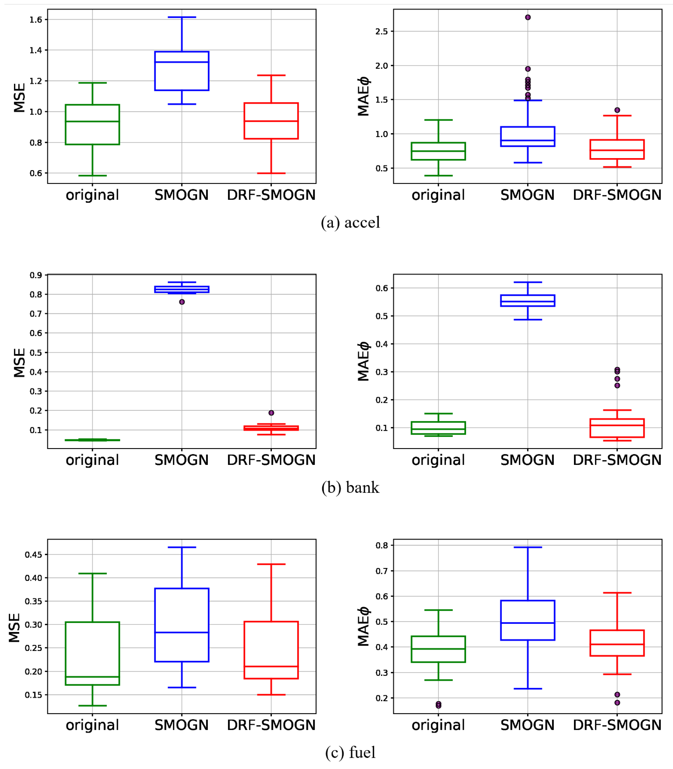
4.3.2. Real Data Results

We evaluated 18 benchmark datasets under three sampling strategies—Original, SMOGN, and DRF–SMOGN—using SVR, NNET, XGB, and RF. Each experiment was repeated 100 times with different random seeds and an 80:20 train–test split. Apart from omitting SMAPE, all other settings (hyperparameters, grid search, evaluation metrics) mirror the simulation study.

Table 4. MSE and $\mathrm{MAE}\varphi$ evaluations on 18 real datasets. Each value represents a mean over multiple runs. Standard deviations, which were within a few percent of the means, are omitted for clarity. The best (i.e., lowest) results for each metric and dataset are marked with an asterisk.

Dataset	Algorithm	MSE			MAE$\mathit{\varphi }$
		Original	SMOGN	DRF-SMOGN	Original	SMOGN	DRF-SMOGN
a1	SVR	336.3	428.2	286.7 *	21.2	16.7 *	16.9
	NNET	556.1 *	581.2	563.9	30.0 *	31.0	30.4
	XGB	323.6 *	454.0	443.2	17.7 *	19.8	18.9
	RF	264.2 *	424.0	350.9	15.9 *	17.4	16.0
a2	SVR	116.1	139.6	111.3 *	13.0	10.2 *	11.8
	NNET	140.6 *	150.1	140.9	15.4 *	16.2	15.5
	XGB	137.8 *	164.7	160.7	12.3	12.0	12.0 *
	RF	108.7 *	150.2	133.4	10.7	10.6	10.5 *
a3	SVR	50.6	55.7	43.1 *	9.9	7.5	7.4 *
	NNET	50.1	51.2	48.4 *	9.5	9.4	9.3 *
	XGB	56.4 *	83.9	73.2	7.3 *	7.5	7.5
	RF	47.8 *	75.7	63.0	7.1	7.0	6.6 *
a4	SVR	21.6 *	24.5	22.5	5.2	4.9	4.6 *
	NNET	20.8	21.2	17.8 *	4.6	4.2	4.1 *
	XGB	32.7 *	37.9	37.9	4.5	4.4	4.3
	RF	21.2 *	28.0	23.2	4.4	4.8	4.2 *
a5	SVR	51.7	67.8	50.2 *	8.6	8.2	8.1 *
	NNET	62.9 *	70.5	63.0	10.3	10.7	10.2 *
	XGB	55.9 *	82.3	77.0	8.2 *	8.9	8.6
	RF	51.2 *	82.0	64.0	7.8	8.0	7.4 *
a6	SVR	150.6	152.8	136.6 *	16.8	16.2	15.2 *
	NNET	138.2	143.2	128.4 *	16.5	16.6	15.8 *
	XGB	147.7 *	211.0	189.0	14.4	14.9	14.4 *
	RF	132.3 *	196.2	151.0	13.2	12.5	12.4 *
a7	SVR	28.1	28.9	26.6 *	8.2	7.8	7.7 *
	NNET	26.1 *	35.9	27.5	7.4	7.2	7.1 *
	XGB	34.4 *	50.4	43.7	6.2 *	7.2	6.4
	RF	25.9 *	40.4	33.1	6.2	6.1	5.6 *
abal	SVR	4.9	5.3	4.8 *	2.3	2.2	2.2 *
	NNET	5.2 *	6.3	6.2	2.2	2.0 *	2.3
	XGB	5.5 *	6.2	5.8	2.2	2.1 *	2.2
	RF	4.8 *	5.7	4.8	2.1	2.0 *	2.1
accel	SVR	0.9 *	1.3	0.9	0.8	0.9	0.8 *
	NNET	1.3 *	3.4	1.7	1.0 *	1.5	1.1
	XGB	0.6 *	1.1	0.7	0.5 *	0.8	0.6
	RF	0.8 *	1.3	0.8	0.7 *	0.9	0.7
avail	SVR	194.8	1174.7	186.8 *	11.0 *	33.6	11.4
	NNET	334.7 *	1449.1	1459.6	16.4 *	31.0	35.2
	XGB	22.4 *	368.2	32.3	2.0 *	13.5	2.6
	RF	55.8 *	560.1	57.3	5.6 *	20.1	5.6
bank	SVR	0.05 *	0.83	0.11	0.12 *	0.58	0.13
	NNET	0.05 *	0.83	0.12	0.12 *	0.57	0.14
	XGB	0.05 *	0.83	0.12	0.08 *	0.54	0.08 *
	RF	0.06 *	0.83	0.12	0.08	0.52	0.07 *
bost	SVR	17.3 *	18.5	18.2	3.3 *	3.4	3.4
	NNET	127.5 *	184.1	208.2	10.2 *	12.0	13.0
	XGB	10.5 *	16.0	12.3	2.7 *	3.2	2.8
	RF	11.1 *	15.2	12.1	2.8 *	3.2	2.9
cpu	SVR	65.9 *	118.8	84.8	6.6 *	7.5	7.5
	NNET	1227.2	825.9 *	2586.5	27.9 *	28.7	40.6
	XGB	12.5 *	14.3	14.5	2.7 *	2.9	2.9
	RF	82.0	83.1	72.8 *	3.0	3.1	3.8 *
dAil	SVR	0.32 *	0.45	0.32 *	1.55	1.91	1.47 *
	NNET	0.32 *	0.45	0.33	1.43	1.78	1.35 *
	XGB	0.36	0.48	0.35 *	1.51	2.01	1.47 *
	RF	0.31 *	0.46	0.32	1.53	2.01	1.48 *
dElev	SVR	0.37	0.56	0.36 *	1.16	1.40	1.15 *
	NNET	0.37 *	0.55	0.38	1.19	1.44	1.10 *
	XGB	0.45 *	0.51	0.46	1.16	1.48	1.14 *
	RF	0.38 *	0.50	0.39	1.15	1.46	1.14 *
fuel	SVR	0.23 *	0.29	0.25	0.35 *	0.40	0.36
	NNET	0.45 *	0.78	0.48	0.45 *	0.62	0.49
	XGB	0.19 *	0.35	0.24	0.33 *	0.46	0.36
	RF	0.28 *	0.46	0.31	0.43 *	0.57	0.45
heat	SVR	165.9	144.2 *	166.5	12.9	11.1 *	12.7
	NNET	183.0 *	421.0	527.2	12.9 *	17.6	23.4
	XGB	11.5 *	39.0	17.9	3.1 *	5.6	3.8
	RF	50.5 *	78.4	53.9	7.0 *	8.6	7.2
maxt	SVR	283.9 *	1784.8	369.0	14.2 *	37.2	16.7
	NNET	3518.2 *	4958.3	7282.4	53.6 *	64.3	90.0
	XGB	31.4 *	759.0	45.8	2.2 *	20.2	2.9
	RF	45.3 *	1204.3	61.7	4.5 *	29.4	5.1

present the mean results for MSE and $\mathrm{MAE}\varphi$. As the standard deviations were within a few percent of the means, they were omitted. Under MSE, the Original approach most often yields the lowest error, with DRF–SMOGN a close second and SMOGN frequently failing to improve—and sometimes degrading—the overall performance. The differences among the methods based on SMAPE results exhibited a similar pattern to those based on MSE, and were therefore omitted for brevity.

When focusing on rare-target accuracy via $\mathrm{MAE}\varphi$, DRF–SMOGN outperforms both Original and SMOGN in the majority of cases, demonstrating its superior ability to predict high-relevance observations. Where the Original approach is marginally better, the gap is small; SMOGN occasionally edges out DRF–SMOGN but only inconsistently and by narrow margins.

Among the four learners, SVR and NNET generally perform best, although NNET’s results can degrade on datasets with many nominal features—highlighting SVR’s robustness across heterogeneous real-world tasks. In summary, DRF–SMOGN maintains the Original dataset’s overall accuracy while substantially improving rare-data predictions, whereas SMOGN’s unimodal assumptions hamper its effectiveness on more complex distributions.

Figure 5 presents boxplots of both MSE and $\mathrm{MAE}\varphi$ for the three selected datasets. We focus on SVR’s results, as its trends mirror those of other learners and it achieves the most stable performance overall. In the ‘bank’ dataset, SMOGN’s MSE errors are substantially higher than those of the Original data, whereas DRF-SMOGN closely matches the Original performance. The $\mathrm{MAE}\varphi$ plots likewise show DRF-SMOGN maintaining parity with the Original, while SMOGN remains suboptimal. Although ‘accel’ and ‘bank’ exhibit slight $\mathrm{MAE}\varphi$ improvements under DRF-SMOGN, the ‘fuel’ dataset does not, highlighting how distributional characteristics can influence sampling efficacy.

When evaluating on real datasets, two factors in particular can affect the performance:

• Nominal features: Unlike our simulations, some real datasets include up to 13 categorical predictors. HEOM handles these by treating each mismatched category as distance 1, which can overwhelm the Euclidean contributions from numerical features when categories dominate. Since DRF-SMOGN weights synthetic targets by inverse distance, overly coarse categorical distances may distort both neighbor selection and target interpolation.
• Gaussian noise sampling: SMOGN’s safety threshold rule falls back on adding Gaussian noise when neighbors are too far apart—a useful idea in principle, but one that depends on a user-defined perturbation constant. Without clear guidelines for setting this constant across diverse datasets, noise levels can vary unpredictably, undermining the stability. The systematic calibration of this parameter—or the adoption of alternative noise models—could yield more consistent results.

Overall, DRF-SMOGN tends to offer more stable and reliable improvements over SMOGN—both on bimodal (simulation) and unimodal (real) data—while often preserving the Original data’s accuracy. Using standard metrics such as MSE and $\mathrm{MAE}\varphi$ allows for a balanced evaluation of performance across the entire distribution.

5. Conclusions

This paper introduces the Distance-based Relevance Function (DRF), a parameter-free approach to imbalanced regression that quantifies target rarity via pairwise distances among standardized values. Unlike box-plot or density-based methods, DRF requires no distributional assumptions and applies broadly to both unimodal and bimodal targets. Integrated into SMOGN, DRF-SMOGN often improves the performance on both synthetic and real-world datasets.

Overall, DRF enables resampling across diverse target distributions without additional tuning. Our evaluation framework highlights both its benefits and the limitations of existing methods—particularly the instability of Gaussian-noise sampling in SMOGN with many nominal features. Future work may explore advanced distance metrics for mixed-type data and refined noise or interpolation strategies to further enhance sample quality.

References

1. Chawla, N.; Bowyer, K.; Hall, L.; Kegelmeyer, W. SMOTE: Synthetic Minority Over-sampling Technique. J. Artif. Intell. Res. 2002, 16, 321–357. [Google Scholar] [CrossRef]
2. King, G.; Zeng, L. Logistic regression in rare events data. Political Anal. 2001, 9, 137–163. [Google Scholar] [CrossRef]
3. Torgo, L.; Ribeiro, R.P. Utility-based regression. In Proceedings of the 11th European Conference on Principles and Practice of Knowledge Discovery in Databases, Warsaw, Poland, 17–21 September 2007; pp. 597–604. [Google Scholar]
4. Torgo, L.; Ribeiro, R.P.; Pfahringer, B.; Branco, P. SMOTE for regression. In Proceedings of the EPIA 2013: Progress in Artificial Intelligence, Azores, Portugal, 9–12 September 2013; pp. 378–389. [Google Scholar]
5. Branco, P.; Torgo, L.; Ribeiro, R.P. SMOGN: A pre-processing approach for imbalanced regression. In Proceedings of the First International Workshop on Learning with Imbalanced Domains: Theory and Applications, Skopje, Macedonia, 22 September 2017; Volume 74, pp. 36–50. [Google Scholar]
6. Steininger, M.; Kobs, K.; Davidson, P.; Krause, A.; Hotho, A. Density-based weighting for imbalanced regression. Mach. Learn. 2021, 110, 2187–2211. [Google Scholar] [CrossRef]
7. Son, J. KSMOTER: KDE SMOTE for Imbalanced Regression. Master’s Thesis, Yonsei University, Seoul, Republic of Korea, 2023. [Google Scholar]
8. Camacho, L.; Douzas, G.; Bacao, F. Geometric SMOTE for regression. Expert Syst. Appl. 2022, 193, 116387. [Google Scholar] [CrossRef]
9. Yang, Y.; Zha, K.; Chen, Y.; Wang, H.; Katabi, D. Delving into deep imbalanced regression. In Proceedings of the 38th International Conference on Machine Learning, Virtual, 18–24 July 2021; pp. 11842–11851. [Google Scholar]
10. Gonzalez-Abril, L.; Guerrero-Gonzalez, A.; Torres, J.; Ortega, J.A. A review on imbalanced data preprocessing for supervised learning: Evolutionary fuzzy systems and beyond. Appl. Sci. 2020, 10, 4014. [Google Scholar]
11. Branco, P.; Torgo, L.; Ribeiro, R.P. Relevance-based evaluation metrics for multi-target regression. Mach. Learn. 2017, 106, 1779–1800. [Google Scholar]
12. Torgo, L.; Ribeiro, R.P. Precision and recall for regression. In Proceedings of the DS 2009: Discovery Science, Porto, Portugal, 3–5 October 2009; pp. 332–346. [Google Scholar]
13. Song, X.Y.; Dao, N.; Branco, P. DistSMOGN: Distributed SMOGN for imbalanced regression problems. In Proceedings of the Fourth International Workshop on Learning with Imbalanced Domains: Theory and Applications, Grenoble, France, 23 September 2022; Volume 183, pp. 38–52. [Google Scholar]
14. Wilson, D.L.; Martinez, T.R. Improved Heterogeneous Distance Functions. In Proceedings of the Fourteenth International Conference on Machine Learning (ICML). Morgan Kaufmann, Nashville, Tennessee, 8–12 July 1997; pp. 656–666. [Google Scholar]
Figure 1. Histogram of target values, corresponding DRF-derived relevance scores for each observation, and the resulting relevance function via cubic Hermite interpolation.
Stats 08 00053 g001
Figure 2. Histograms of simulation training (bimodal) and test (unimodal) datasets.
Stats 08 00053 g002
Figure 3. Histograms and DRF relevance score curves for training data across different α values. Denser regions receive lower raw scores and thus lower relevance, while isolated regions near the median gap yield higher relevance.
Stats 08 00053 g003
Figure 4. MSE comparison for (a) SVR and (b) NNET on simulation datasets.
Stats 08 00053 g004
Figure 5. Boxplots of MSE and MAE ϕ over 100 runs on real datasets (a) accel, (b) bank, and (c) fuel using Support Vector Regressor.
Stats 08 00053 g005