A Smoothed Three-Part Redescending M-Estimator

Abstract

A smoothed M-estimator is derived from Hampel’s three-part redescending estimator for location and scale. The estimator is shown to be weakly continuous and Fréchet differentiable in the neighbourhood of the normal distribution. Asymptotic assessment is conducted at asymmetric contaminating distributions, where smoothing is shown to improve variance and change-of-variance sensitivity. Other robust metrics compared are largely unchanged, and therefore, the smoothed functions represent an improvement for asymmetric contamination near the rejection point with little downside.

1. Introduction

In this paper, we describe a refinement of the Hampel three-part redescenders [1] that smooths sharp corners in the spirit of [2,3]. In doing so, all the asymptotic theories of weak continuity and Fréchet differentiability apply to the introduced M-estimators. The central parametric family studied here is assumed to be

$$\mathcal{F}=\left\{F_{{(\mu ,\sigma )}^{\top }}\left(x\right)=\Phi \left({\displaystyle \frac{x-\mu }{\sigma }}\right):-\infty <\mu <\infty ,\sigma >0\right\},$$

where $\Phi \left(x\right)$ is the standard cumulative normal distribution on the real line. Without loss of generality estimators including M-estimators described in [4,5,6], it can be studied at the standard normal distribution where ${(\mu ,\sigma )}^{\top }={(0,1)}^{\top }$. This paper differs from many in that the asymptotics and the performance of estimators are discussed in a neighbourhood of underlying distributions. The main distribution is standard normal, with a contamination parameterised by ${\mu }_2$ and $\alpha$, as follows:

$$G_0\left(x\right)=(1-ϵ)\Phi \left(x\right)+ϵ\Phi \left({\displaystyle \frac{x-{\mu }_2}{\alpha }}\right),$$

(1)

where $0<ϵ<1/2$ is considered small, ${\mu }_2\in \mathbb{R}$ (the real line), and $\alpha \in {\mathbb{R}}^{+}$. The distribution is symmetric when ${\mu }_2=0$ and asymmetric otherwise. Contamination processes themselves may be subject to the central limit theorem, whence the mixture model is apt. Moreover, regarding alternative heavy-tailed contamination, this may be represented by choosing ${\mu }_2$ to be arbitrarily large. Since there is no restriction placed on ${\mu }_2$ and $\alpha$, very large outliers can be represented using the mixture.

In a sense [1], following the publication of [7], contaminated populations with the description of a rejection point are predicated, beyond which observations are to have zero weight on the estimation procedure. This came accompanying the introduction of the first $\psi$-function in robust estimation to continuously redescend to zero, as follows:

$${\psi }_{1;a,b,c}\left(x\right)=\left\{\begin{array}{cc}x\hfill & \mathrm{for}0\le \left|x\right|\le a\hfill \\ asign\left(x\right)\hfill & \mathrm{for}a\le \left|x\right|\le b\hfill \\ a{\displaystyle \frac{c-\left|x\right|}{c-b}}sign\left(x\right)\hfill & \mathrm{for}b\le \left|x\right|\le c\hfill \\ 0\hfill & \mathrm{for}c\le \left|x\right|\hfill \end{array}\right.,$$

(2)

where $0<a\le b\le c$. The tuning constant a defines a region about which the estimator is equivalent to the maximum likelihood estimate at $\mathcal{F}=\Phi$, $\psi \left(x\right)=x$. The value of b can be used to “Winsorise” the observations between a and b standard deviations from the true location. The rejection point is set by the tuning constant c. Figure 1 plots ${\psi }_{1;a,b,c}$. Setting $b=c=\infty$ yields Huber’s $\psi$-function. See [8].

The study of the Hampel three-part redescender considered estimating location only and made use of an auxiliary estimator of scale. The work in [1,8,9,10] addresses the question of the scale of the central distribution by suggesting using either a robust estimator of scale such as the median of the absolute deviations (MAD) estimator or its consistent version, that is,

$$MADN=median\left\{\right|X_i-median(X_1,X_2,\dots ,X_n)\left|\right\}/0.6745,$$

where the value 0.6745 is to make the scale estimator consistent for the scale when the underlying distribution is indeed normal. See [11] for a recent synthesis of MADN. The estimator of location is then solved via a scaled location equation. Given the sample $X_1,X_2,\dots X_n$ from a hypothesised distribution in $\mathcal{F}$ and an estimate of the standard deviation $\sigma$, say, $\widehat{\sigma }$, the estimating equation for location is then of the form

$$\sum _{i=1}^n{\psi }_{1;a,b,c}\left({\displaystyle \frac{X_i-\mu }{\widehat{\sigma }}}\right)=0.$$

Alternatively, the estimator of both location and scale can be solved through the use of the solution of the simultaneous equations

$${\mathbf{K}}_{\mathbf{n}}({\tau }_1,{\tau }_2)={\displaystyle \frac{1}{n}}\sum _{i=1}^n\mathbf{\Psi }\left({\displaystyle \frac{X_i-{\tau }_1}{{\tau }_2}}\right)=\int \mathbf{\Psi }\left({\displaystyle \frac{x-{\tau }_1}{{\tau }_2}}\right)d{F}_n\left(x\right)=\mathbf{0}.$$

(3)

Here, $F_n\left(x\right)$ is the empirical distribution of the sample, and $\mathbf{\Psi }={\left({\psi }_1,{\psi }_2\right)}^{\top }$ is a vector function used in the estimation for location and scale. In this work, we propose estimators for both location and scale and, as such, focus on joint estimation. A three-part redescending M-estimator of scale may be constructed in the following form:

$${\psi }_{2;a,b,c}\left(x\right)=\left\{\begin{array}{cc}{x}^2-1-P\hfill & \mathrm{for}0\le \left|x\right|\le a\hfill \\ a^2-1-P\hfill & \mathrm{for}a\le \left|x\right|\le b\hfill \\ (a^2-1-P){\displaystyle \frac{c-\left|x\right|}{c-b}}\hfill & \mathrm{for}b\le \left|x\right|\le c\hfill \\ 0\hfill & \mathrm{for}c\le \left|x\right|\hfill \end{array}\right.,$$

(4)

where P is defined implicitly from the equation $\int {\psi }_{2;a,b,c}\left(x\right)d\Phi \left(x\right)=0$. See, for example, [12]. Setting $b=c=\infty$ yields Huber’s Proposal 2 estimator for scale, defined in [8]. Equation (4) is illustrated in Figure 1. Then to obtain the estimator, one solves (3) with $\mathbf{\Psi }={\mathbf{\Psi }}_{a,b,c}={({\psi }_{1;a,b,c},{\psi }_{2;a,b,c})}^{\top }$. Note that these functions are continuous but not smooth at $a,b$, and c.

Important robustness properties are a result of Fréchet differentiability, including uniform asymptotic consistency of the estimate’s variability assessment based on the influence function. See [2]. Proofs of Fréchet differentiability in the neighbourhood of a central distribution are challenging for non-smooth $\psi$ functions; hence, smoothing to achieve a proof of Fréchet differentiability is desirable.

The remainder of this paper is structured as follows: In Section 2.1, we describe the smoothed M-estimator. Section 2.2 describes Fréchet differentiability and introduces theorems necessary to prove weak continuity and Fréchet differentiability of the introduced estimator. Additional robustness measures are introduced in Section 2.3, before comparing the smoothed and non-smoothed variants against these measures and considering their asymptotic behaviour at $G_0$ in Section 3.

2. Materials and Methods

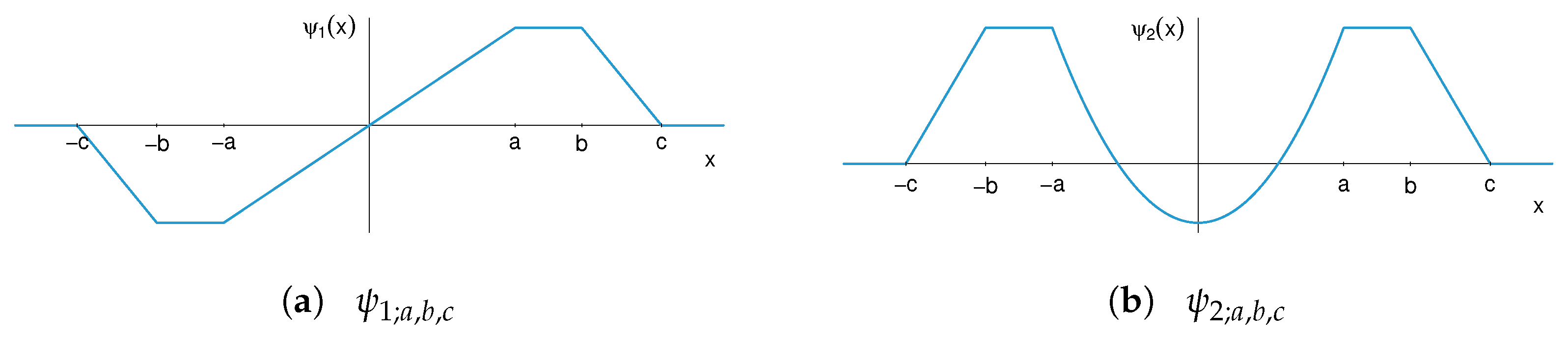
2.1. A Smoothed Three-Part Redescender

The Hampel three-part redescending $\psi$-functions are continuous but not continuously differentiable at $x=i\in \left\{\pm a,\pm b,\pm c\right\}$. To rectify this, one may insert smoothing functions in the $2\delta$ neighbourhood of each i, where $\delta \le min{\displaystyle \frac{1}{2}}\left\{a,b-a,c-b\right\}$. As the three-part redescender is defined in terms of piecewise polynomials with heuristic tuning constants, it is desirable to retain the same properties while attaining twice differentiable functions such that higher-order asymptotics could be explored in later works. Interpolation methods, such as that outlined by ([13] p. 319), may be extended to fifth-degree polynomials, $g_{ji}\left(x\right)$, with the following constraints to ensure the resultant $\psi$ functions are twice differentiable:

$$\begin{array}{cc}\hfill g_{ji}(i-\delta )& ={\psi }_{j;a,b,c}(i-\delta )\hfill \\ \hfill g_{ji}(i+\delta )& ={\psi }_{j;a,b,c}(i+\delta )\hfill \\ \hfill g_{ji}^{\prime }(i-\delta )& ={\psi }_{j;a,b,c}^{\prime }(i-\delta )\hfill \\ \hfill g_{ji}^{\prime }(i+\delta )& ={\psi }_{j;a,b,c}^{\prime }(i+\delta )\hfill \\ \hfill g_{ji}^{\prime \prime }(i-\delta )& ={\psi }_{j;a,b,c}^{\prime \prime }(i-\delta )\hfill \\ \hfill g_{ji}^{\prime \prime }(i+\delta )& ={\psi }_{j;a,b,c}^{\prime \prime }(i+\delta )\hfill \end{array}$$

where ${\psi }_{j;a,b,c}$ for $j\in \left\{1,2\right\}$ denotes Hampel’s location and Clarke and Milne’s scale functions for the three-part redescender with $a,b$, and c as given in [12]. From these boundary conditions, it is simple to formulate and solve a system of linear equations, as follows:

$${\mathbf{A}}_{ji}{\mathbf{x}}_{ji}={\mathbf{b}}_{ji}$$

(5)

to identify the polynomial coefficients ${\mathbf{x}}_{ji}$ for each $g_{ji}\left(x\right)$. Here, ${\mathbf{A}}_{ji}{\mathbf{x}}_{ji}$ represents the left side of the aforementioned constraints, and ${\mathbf{b}}_{ji}$ the right side. For example, the coefficients for

$$\begin{array}{cc}\hfill g_{1a}\left(x\right)& ={\alpha }_{1,5}{x}^5+{\alpha }_{1,4}{x}^4+{\alpha }_{1,3}{x}^3+{\alpha }_{1,2}{x}^2+{\alpha }_{1,1}x+{\alpha }_{1,0}\hfill \\ \hfill g_{1a}^{\prime }\left(x\right)& =5{\alpha }_{1,5}{x}^4+4{\alpha }_{1,4}{x}^3+3{\alpha }_{1,3}{x}^2+2{\alpha }_{1,2}x+{\alpha }_{1,1}\hfill \\ \hfill g_{1a}^{″}\left(x\right)& =20{\alpha }_{1,5}{x}^3+12{\alpha }_{1,4}{x}^2+6{\alpha }_{1,3}x+2{\alpha }_{1,2}\hfill \end{array}$$

are the solution of (5), where

$$\begin{array}{cc}\hfill {\mathbf{A}}_{1a}& =\left[\begin{array}{cccccc}{(a-\delta )}^5& {(a-\delta )}^4& {(a-\delta )}^3& {(a-\delta )}^2& (a-\delta )& 1\\ {(a+\delta )}^5& {(a+\delta )}^4& {(a+\delta )}^3& {(a+\delta )}^2& (a+\delta )& 1\\ 5{(a-\delta )}^4& 4{(a-\delta )}^3& 3{(a-\delta )}^2& 2(a-\delta )& 1& 0\\ 5{(a+\delta )}^4& 4{(a+\delta )}^3& 3{(a+\delta )}^2& 2(a+\delta )& 1& 0\\ 20{(a-\delta )}^3& 12{(a-\delta )}^2& 6(a-\delta )& 2& 0& 0\\ 20{(a+\delta )}^3& 12{(a+\delta )}^2& 6(a+\delta )& 2& 0& 0\end{array}\right],\hfill \\ \hfill {\mathbf{x}}_{1a}& ={\left[\begin{array}{cccccc}{\alpha }_{1,5}& {\alpha }_{1,4}& {\alpha }_{1,3}& {\alpha }_{1,2}& {\alpha }_{1,1}& {\alpha }_{1,0}\end{array}\right]}^T,\hfill \end{array}$$

and

$$\begin{array}{c}\hfill {\mathbf{b}}_{1a}=\left[\begin{array}{c}{\psi }_{1;a,b,c}(a-\delta )\\ {\psi }_{1;a,b,c}(a+\delta )\\ {\psi }_{1;a,b,c}^{\prime }(a-\delta )\\ {\psi }_{1;a,b,c}^{\prime }(a+\delta )\\ {\psi }_{1;a,b,c}^{\prime \prime }(a-\delta )\\ {\psi }_{1;a,b,c}^{\prime \prime }(a+\delta )\end{array}\right]=\left[\begin{array}{c}(a-\delta )\\ a\\ 1\\ 0\\ 0\\ 0\end{array}\right].\end{array}$$

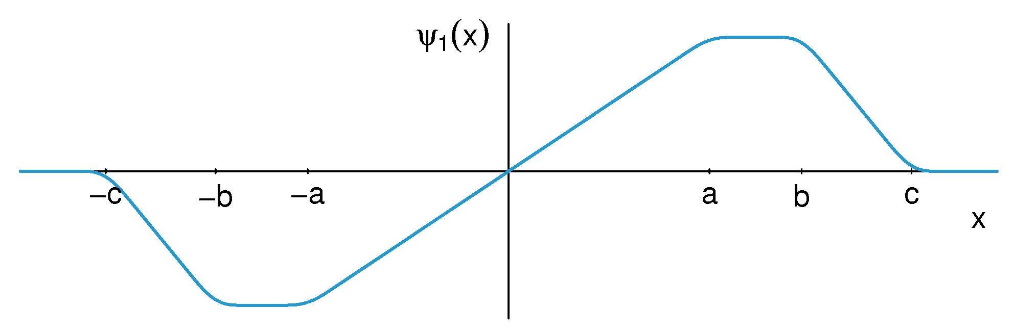
2.1.1. Smoothed Three-Part Redescender for Location

Inserting polynomial smoothing functions in the $2\delta$ regions around a, b, and c yields the following $\psi$ function for location:

$$\begin{array}{cc}\hfill {\psi }_{1;a,b,c,\delta }& =\left\{\begin{array}{cc}x\hfill & \left|x\right|\le (a-\delta )\hfill \\ g_{1a}\left(x\right)\hfill & (a-\delta )<\left|x\right|\le (a+\delta )\hfill \\ asign\left(x\right)\hfill & (a+\delta )\le \left|x\right|\le (b-\delta )\hfill \\ g_{1b}\left(x\right)\hfill & (b-\delta )<\left|x\right|\le (b+\delta )\hfill \\ a{\displaystyle \frac{c-\left|x\right|}{c-b}}sign\left(x\right)\hfill & (b+\delta )\le \left|x\right|\le (c-\delta )\hfill \\ g_{1c}\left(x\right)\hfill & (c-\delta )<\left|x\right|\le (c+\delta )\hfill \\ 0\hfill & \mathrm{otherwise}\hfill \end{array}\right.\hfill \end{array}$$

where

$$\begin{array}{cc}\hfill g_{1a}\left(x\right)& =\left({\alpha }_{1,4}{x}^4+{\alpha }_{1,2}{x}^2+{\alpha }_{1,0}\right)sign\left(x\right)+{\alpha }_{1,3}{x}^3+{\alpha }_{1,1}x\hfill \\ \hfill g_{1b}\left(x\right)& =\left({\beta }_{1,4}{x}^4+{\beta }_{1,2}{x}^2+{\beta }_{1,0}\right)sign\left(x\right)+{\beta }_{1,3}{x}^3+{\beta }_{1,1}x\hfill \\ \hfill g_{1c}\left(x\right)& =\left({\gamma }_{1,4}{x}^4+{\gamma }_{1,2}{x}^2+{\gamma }_{1,0}\right)sign\left(x\right)+{\gamma }_{1,3}{x}^3+{\gamma }_{1,1}x\hfill \end{array}$$

and

$$\begin{array}{cc}\hfill {\alpha }_{1,4}& =\zeta \hfill \\ \hfill {\alpha }_{1,3}& =-4a\zeta \hfill \\ \hfill {\alpha }_{1,2}& =6\left(a^2-{\delta }^2\right)\zeta \hfill \\ \hfill {\alpha }_{1,1}& =-4\left(a^3-3a{\delta }^2-2{\delta }^3\right)\zeta \hfill \\ \hfill {\alpha }_{1,0}& =\left(a^4-6a^2{\delta }^2+8a{\delta }^3-3{\delta }^4\right)\zeta \hfill \end{array}$$

$$\begin{array}{cc}\hfill {\beta }_{1,4}& =-a\xi \hfill \\ \hfill {\beta }_{1,3}& =4ab\xi \hfill \\ \hfill {\beta }_{1,2}& =-6a(b^2-{\delta }^2)\xi \hfill \\ \hfill {\beta }_{1,1}& =4a\left(b^3-3b{\delta }^2+2{\delta }^3\right)\xi \hfill \\ \hfill {\beta }_{1,0}& =-a(b^4-6b^2{\delta }^2-8b{\delta }^3-3{\delta }^4+16c{\delta }^3)\xi \hfill \end{array}$$

$$\begin{array}{cc}\hfill {\gamma }_{1,4}& =a\xi \hfill \\ \hfill {\gamma }_{1,3}& =-4ac\xi \hfill \\ \hfill {\gamma }_{1,2}& =6a\left(c^2-{\delta }^2\right)\xi \hfill \\ \hfill {\gamma }_{1,1}& =-4a(c^3-3c{\delta }^2-2{\delta }^3)\xi \hfill \\ \hfill {\gamma }_{1,0}& =a\left(c^4-6c^2{\delta }^2-8c{\delta }^3-3{\delta }^4\right)\xi \hfill \end{array}$$

for $\zeta ={\left(16{\delta }^3\right)}^{-1}$, and $\xi ={\left(16{\delta }^3(b-c)\right)}^{-1}$. Figure 2 plots the smoothed three-part redescender for location. In this general form, the functional may appear to suffer from too many parameters; however, the coefficients ${\alpha }_{1,·},{\beta }_{1,·},{\gamma }_{1,·}$ are wholly dependent upon $a,b,c,$ and $\delta$. The resultant $\psi$-function is piecewise polynomial.

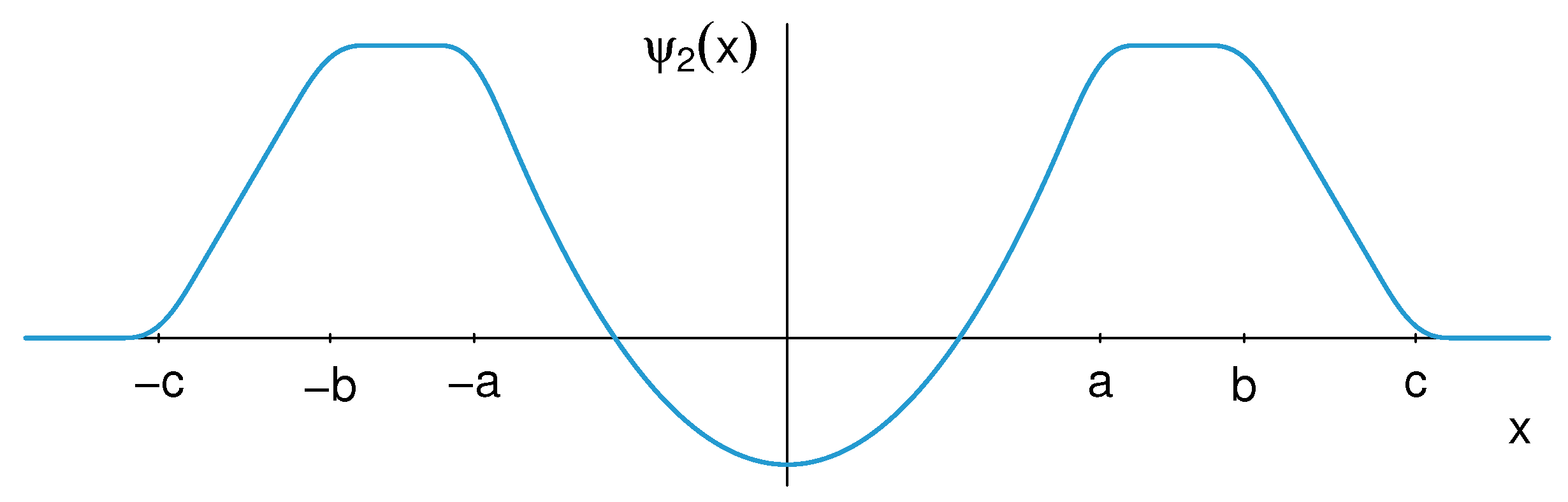
2.1.2. Smoothed Three-Part Redescender for Scale

The smoothing procedure for the scale $\psi$ function yields the following definition:

$$\begin{array}{cc}\hfill {\psi }_{2;a,b,c,\delta }& =\left\{\begin{array}{cc}{x}^2-1-P\hfill & \left|x\right|\le (a-\delta )\hfill \\ g_{2a}\left(x\right)\hfill & (a-\delta )\le \left|x\right|\le (a+\delta )\hfill \\ \eta \hfill & (a+\delta )\le \left|x\right|\le (b-\delta )\hfill \\ g_{2b}\left(x\right)\hfill & (b-\delta )<\left|x\right|\le (b+\delta )\hfill \\ \eta {\displaystyle \frac{c-\left|x\right|}{c-b}}\hfill & (b+\delta )\le \left|x\right|\le (c-\delta )\hfill \\ g_{2c}\left(x\right)\hfill & (c-\delta )\le \left|x\right|\le (c+\delta )\hfill \\ 0\hfill & \mathrm{otherwise}\hfill \end{array}\right.\hfill \end{array}$$

where

$$\begin{array}{cc}\hfill g_{2a}\left(x\right)& =\left({\alpha }_{2,5}{x}^5+{\alpha }_{2,3}{x}^3+{\alpha }_{2,1}x\right)sign\left(x\right)\hfill \\ \hfill & +{\alpha }_{2,4}{x}^4+{\alpha }_{2,2}{x}^2+{\alpha }_{2,0}\hfill \\ \hfill g_{2b}\left(x\right)& ={\beta }_{2,4}{x}^4+{\beta }_{2,2}{x}^2+\left({\beta }_{2,3}{x}^3+{\beta }_{2,1}x\right)sign\left(x\right)+{\beta }_{2,0}\hfill \\ \hfill g_{2c}\left(x\right)& ={\gamma }_{2,4}{x}^4+{\gamma }_{2,2}{x}^2+\left({\gamma }_{2,3}{x}^3+{\gamma }_{2,1}x\right)sign\left(x\right)+{\gamma }_{2,0}\hfill \end{array}$$

and

$$\begin{array}{cc}\hfill {\alpha }_{2,5}& =\zeta \hfill \\ \hfill {\alpha }_{2,4}& =-3a\zeta \hfill \\ \hfill {\alpha }_{2,3}& =2(a^2-3{\delta }^2)\zeta \hfill \\ \hfill {\alpha }_{2,2}& =2(a^3+3a{\delta }^2+4{\delta }^3)\zeta \hfill \\ \hfill {\alpha }_{2,1}& =-3(a^4-2a^2{\delta }^2+{\delta }^4)\zeta \hfill \\ \hfill {\alpha }_{2,0}& =-\left(16P{\delta }^3+3a{\delta }^4-a^5+16{\delta }^3-8a^2{\delta }^3+6a^3{\delta }^2\right)\zeta \hfill \end{array}$$

$$\begin{array}{cc}\hfill {\beta }_{2,4}& =-\eta \xi \hfill \\ \hfill {\beta }_{2,3}& =4b\eta \xi \hfill \\ \hfill {\beta }_{2,2}& =-6(b^2-{\delta }^2)\eta \xi \hfill \\ \hfill {\beta }_{2,1}& =4(b^3+2{\delta }^3-3b{\delta }^2)\eta \xi \hfill \\ \hfill {\beta }_{2,0}& =\left(6b^2{\delta }^2+8b{\delta }^3-16c{\delta }^3+3{\delta }^4-b^4\right)\eta \xi \hfill \end{array}$$

$$\begin{array}{cc}\hfill {\gamma }_{2,4}& =\eta \xi \hfill \\ \hfill {\gamma }_{2,3}& =-4c\eta \xi \hfill \\ \hfill {\gamma }_{2,2}& =6(c^2-{\delta }^2)\eta \xi \hfill \\ \hfill {\gamma }_{2,1}& =4(2{\delta }^3-c^3+3c{\delta }^2)\eta \xi \hfill \\ \hfill {\gamma }_{2,0}& =-(3{\delta }^4-c^4+6c^2{\delta }^2+8c{\delta }^3)\eta \xi \hfill \end{array}$$

for $\zeta ={\left(16{\delta }^3\right)}^{-1}$ and $\xi ={\left(16{\delta }^3(b-c)\right)}^{-1}$, as before, and $\eta =a^2-1-P$. Once again, the coefficients ${\alpha }_{2,·},{\beta }_{2,·},{\gamma }_{2,·}$ are not free variables; they are dependent upon $a,b,c,$ and $\delta$.

As for the non-smoothed three-part redescender, P may be found as the root of the implicit equation $\int {\psi }_2\left(x\right)\varphi \left(x\right)dx=0$, or can be expanded to an explicit form in terms of the standard normal distribution pdf and cdf (as shown in the Supplementary Materials). Figure 3 plots the above smoothed function for scale.

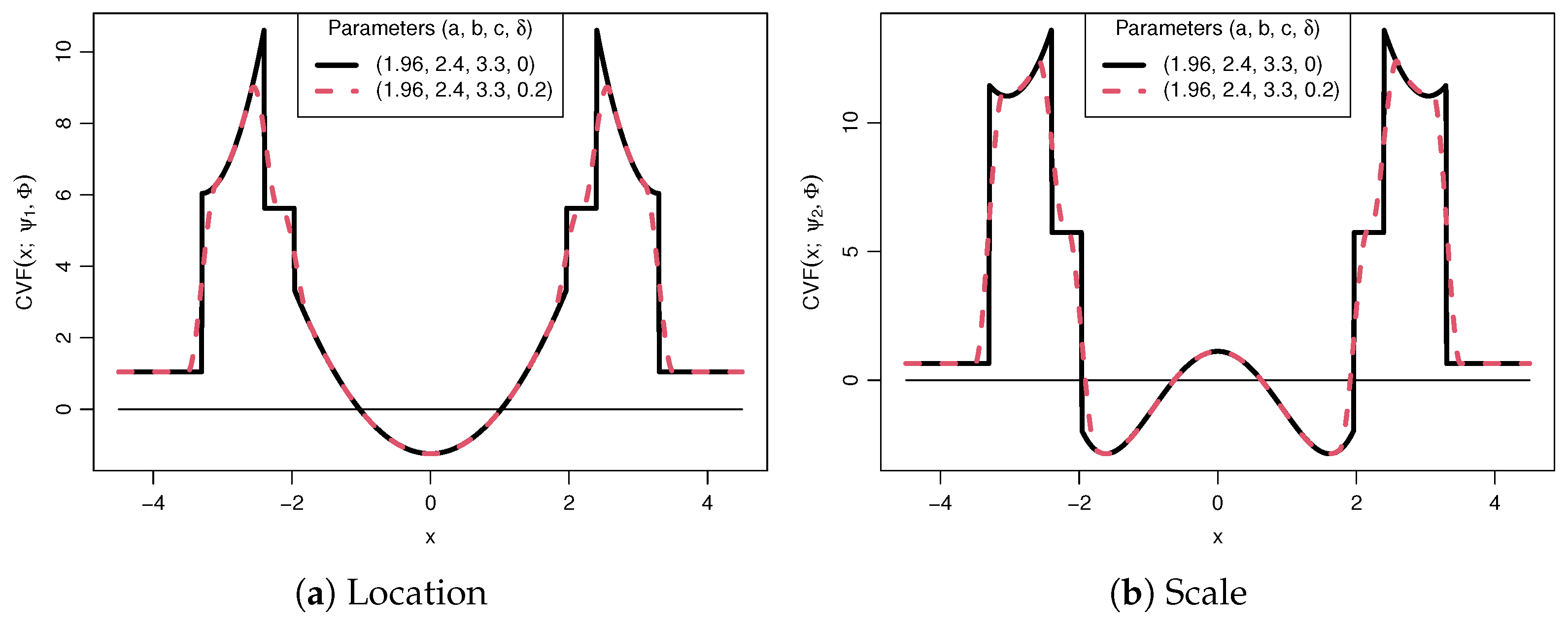
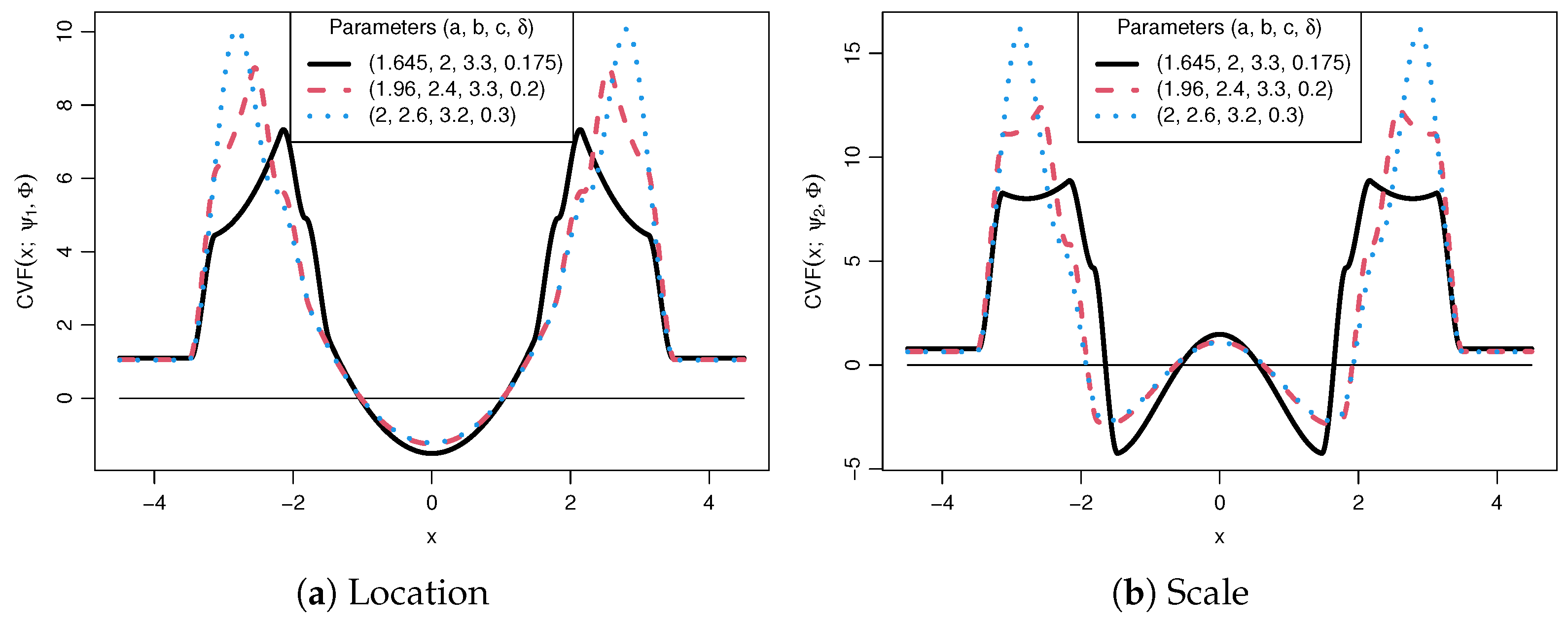
2.2. The Influence Function and Fréchet Derivative

To compare robustness and the behaviour of estimators, one requires appropriate measures and tools. The estimator, which is a solution of Equation (3), is related here in its implicit functional form. Quoting from [6] (p. 29), where now $\mathcal{F}$ is any suitable parametric family, “A single functional root of Equation (3) may be written $\mathbf{T}[\mathbf{\Psi },F_n]$ where $F_n$ is the empirical distribution function. More generally $\mathbf{T}[\mathbf{\Psi },G]$ can be defined as a functional root of equations

$${\mathbf{K}}_G\left(\mathit{\tau }\right)={\int }_{\mathbb{R}}\mathbf{\Psi }(x,\mathit{\tau })dG\left(x\right)=\mathbf{0}.$$

(6)

$\mathbf{T}[\mathbf{\Psi },G]=+\infty$ if no root exists. In the event of several roots of (6), a distance criterion ${\rho }_o$ is employed to select the estimator from them. Classically, the roots correspond to extremes of the distance, but this is not assumed here. Specifically, the general functional $\mathbf{T}[\mathbf{\Psi },{\rho }_o,·]$ is defined as the solution to

$$\underset{\mathit{\tau }\in S(\mathbf{\Psi },G)}{inf}{\rho }_o(G,\mathit{\tau })={\rho }_o(G,\mathbf{T}[\mathbf{\Psi },{\rho }_o,G]),$$

(7)

where

$$S(\mathbf{\Psi },G)=\left\{\mathit{\tau }\in \mathcal{T}\left|{\int }_{\mathbb{R}}\mathbf{\Psi }(x,\mathit{\tau })dG\left(x\right)=\mathbf{0}\right.\right\},$$

(8)

if a solution exists. Otherwise $\mathbf{T}[\mathbf{\Psi },{\rho }_o,G]=+\infty .$ Conditions on both $\mathbf{\Psi }$ and ${\rho }_o$ determine consistency, the very minimum requirement being Fisher consistency, which means that $\mathbf{T}[\mathbf{\Psi },{\rho }_o,F_{\mathit{\tau }}]=\mathit{\tau }$ for all $\mathit{\tau }\in \mathcal{T}$. That is if you have the whole population you must get the corresponding true parameter. This implicitly also assumes the parametric model for the population is identifiable. A parametric family $\mathcal{F}$ is identifiable if and only if $F_{{\mathit{\tau }}_{\mathbf{1}}}=F_{{\mathit{\tau }}_{\mathbf{2}}}$ implies ${\mathit{\tau }}_{\mathbf{1}}={\mathit{\tau }}_{\mathbf{2}}$ for all ${\mathit{\tau }}_{\mathbf{1}},{\mathit{\tau }}_{\mathbf{2}}\in \mathcal{T}.$ That is, two different parameters cannot give the same distribution”.

An easily afforded selection functional ${\rho }_o$ at the location and scale parametric model is

$${\rho }_o(G,\mathit{\tau })={∥\mathit{\tau }-{\left[G^{-1}\left({\displaystyle \frac{1}{2}}\right),MADN\left(G\right)\right]}^{\top }∥}^2$$

(9)

Here, $\parallel ·\parallel$ is the Euclidean norm. The functional form of MADN and the influence function of MAD are discussed in [10] Section 5.2 and also [11,14].

First introduced by [1,15], the Influence Function (IF) is a heuristic tool that indicates the infinitesimal influence of contamination at a given point, $x=z_0$, on the asymptotic value $\mathbf{T}[\psi ,G_0]$. In our discussion, ${\mathit{\tau }}_{\mathbf{0}}=\mathbf{T}[\mathbf{\Psi },{\rho }_o,{\mathbf{G}}_{\mathbf{0}}]$. For the estimating functional $\mathbf{T}$ at a distribution $G_0$, the IF is defined as

$$\mathbf{IF}(z_0;G_0,\mathbf{T})=\underset{\epsilon \to 0^{+}}{lim}{\displaystyle \frac{\mathbf{T}[(1-\epsilon )G_0+\epsilon {\Delta }_{z_0}]-\mathbf{T}\left[G_0\right]}{\epsilon }}$$

(10)

where ${\Delta }_{z_0}$ puts mass 1 at the point $z_0$. In [5,16], the authors write an equivalent definition, as follows:

$$\mathbf{IF}(z_0;G_0,\mathbf{T})=-\mathbf{M}{\left({\mathit{\tau }}_0,G_0\right)}^{-1}\mathbf{\Psi }\left(z_0,{\mathit{\tau }}_0\right).$$

(11)

The matrix

$$\mathbf{M}({\mathit{\tau }}_0,G_0)={\int }_{\mathbb{R}}{\left.\left\{{\displaystyle \frac{\partial }{\partial \mathit{\tau }}}\mathbf{\Psi }(x,\mathit{\tau })\right\}\right|}_{\mathit{\tau }={\mathit{\tau }}_{\mathbf{0}}}d{G}_0\left(x\right)$$

(12)

is assumed to be nonsingular. In this form, we see that the Influence Function is proportional to $\mathbf{\Psi }$, and indeed, the Fréchet derivative in Theorem 2 to be expressed below is exactly

$${\mathbf{T}}_{G_0}^{\prime }(G-G_0)={\int }_{\mathbb{R}}\mathbf{IF}(x;G_0,\mathbf{T})d(G-G_0)\left(x\right).$$

See [17] for an earlier chronological account of the development of the Fréchet derivative in statistics.

So long as we have a compact set D that excludes the solution for scale ${\tau }_2=0$ in which we search for the roots, the conditions set out below are easy to check and are sufficient to provide weak continuity and Fréchet differentiability.

• Conditions  $\mathcal{W}$

$W_0$:

$\mathbf{T}[\mathbf{\Psi },{\rho }_0,G_0]={\mathit{\tau }}_{\mathbf{0}}$.

$W_1$:

$\mathbf{\Psi }$ is a $2\times 1$ vector function on $\mathbb{R}\times \mathbf{\Theta }$ and has continuous partial derivatives on $\mathbb{R}\times D$, where $D\subset \mathbf{\Theta }$ is some non-degenerate compact interval containing ${\mathit{\tau }}_{\mathbf{0}}={({\mathit{\tau }}_{01},{\mathit{\tau }}_{02})}^{\top }$ in its interior and for which the scale ${\mathit{\tau }}_{02}$ is bounded away from zero.

$W_2$:

$\left\{\mathbf{\Psi }(x,\mathit{\tau })|\mathit{\tau }\in D\right\}$, $\left\{{\displaystyle \frac{\partial }{\partial \mathit{\tau }}}\mathbf{\Psi }(x,\mathit{\tau })|\mathit{\tau }\in D\right\}$ are bounded above in Euclidean norm $\left|\mathbf{A}\right|={\left\{\mathrm{trace}\left({\mathbf{A}}^{\mathbf{T}}\mathbf{A}\right)\right\}}^{1/2}$ by a constant.

$W_3$:

The matrix $\mathbf{M}\left({\mathit{\tau }}_{\mathbf{0}},G_0\right)$, given by (12), is nonsingular.

The innovation in the conditions made here is to describe the Conditions at $G_0$, rather than an assumed $F_{\mathit{\tau }}$. Note that we discuss the behaviour of the estimating functional at a solution $\mathbf{T}[\mathbf{\Psi },{\rho }_0,G_0]={\mathit{\tau }}_{\mathbf{0}}$ different from $\mathbf{T}[\mathbf{\Psi },{\rho }_0,F_{\mathit{\tau }}]=\mathit{\tau }$. The restriction to a compact set D is for convenience rather than necessity, since it is easier to check the conditions. Since $G_0$ is chosen to be from the mixture distribution (1) which has for any given $G_0$ a bounded density and is an absolutely continuous distribution, the Conditions $\mathcal{W}$ imply Conditions $\mathcal{A}$ analogous to those defined in [6] (pp. 31,32) for the neighbourhoods generated by any one of the metric distances, these being Kolmogorov (also known as the Kolmogorov–Smirnov), Lévy, or Prohorov metrics. For example, the Kolmogorov–Smirnov metric or supremum norm between the two distributions F and G defined on the real line is $d_{KS}(F,G)={sup}_x|F\left(x\right)-G\left(x\right)|$. At an absolutely continuous distribution $G_0$ with a density that is bounded by a constant $C>0$, it is noted, compare [6] problem 2.3, as follows:

$$d_{KS}(G,G_0)\le (C+1)d_L(G,G_0)\le (C+1)d_P(G,G_0),$$

where $d_L$ is the Lévy metric and $d_P$ is the Prohorov metric. The Prohorov metric governs the weak topology, as discussed in [18], and it is known that the empirical distribution generated by $G_0$ converges weakly to $G_0$ on a set of probability one. Hence, for a weakly continuous estimator, that is, an estimator that is continuous with respect to the Prohorov metric, we have automatic consistency, as explained further below. Moreover, the smoothed M-estimators discussed in this paper will be robust at $G_0$ in the sense of Theorem 2 of [18], as demonstrated in Theorem 2.5 and Corollary 2.3 in [6].

However, for $\mathbf{\Psi }$ choices with continuous partial derivatives, as is the case of $\mathbf{\Psi }={\left({\psi }_{1;a,b,c,\delta },{\psi }_{2;a,b,c,\delta }\right)}^{\top }$, and noting that the functions are of total bounded variation, we can claim the existence of a weakly continuous and Fréchet differentiable root as a corollary to [6] [Theorem 2.3, Theorem 2.6] and [6] [Theorem 2.5] using the auxiliary selection functional $\rho (G,\mathit{\tau })=|\mathit{\tau }-{\mathit{\tau }}_{\mathbf{0}}|$.

Theorem 1

(Adapting Theorem 2.5 of [6]). Assume Conditions $\mathcal{W}$. Then for ϵ small and non-negative, there exists a Prohorov neighbourhood $U\left(G_0\right)$ of $G_0$ such that the functional defined via $\mathbf{T}[\mathbf{\Psi },\rho ,·]$ is weakly continuous at each $G\in U\left(G_0\right)$.

See Appendix A for the proof of Theorem 1. In addition, we can write

Theorem 2

(Adapting Theorem 2.6 of [6]). Assume Conditions $\mathcal{W}$ and assume for all $G\in \mathcal{G}$, the space of distributions on the real line, that

$${\int }_{\mathbb{R}}\mathbf{\Psi }(x,{\mathit{\tau }}_{\mathbf{0}})d(G-G_0)\left(x\right)=O\left(d_{KS}(G,G_0)\right)$$

(13)

as $d_{KS}(G,G_0)\to 0$. Then

$$\left|\mathbf{T}[\mathbf{\Psi },\rho ,G]-\mathbf{T}[\mathbf{\Psi },\rho ,G_0]-{\mathbf{T}}_{G_0}^{\prime }(G-G_0)\right|=o\left(d_{KS}(G,G_0)\right),$$

where

$${\mathbf{T}}_{G_0}^{\prime }(G-G_0)=-M{({\mathit{\tau }}_{\mathbf{0}},G_0)}^{-1}{\int }_{\mathbb{R}}\mathbf{\Psi }(x,{\mathit{\tau }}_{\mathbf{0}})d(G-G_0)\left(x\right)$$

That is, $\mathbf{T}[\mathbf{\Psi },\rho ,·]$ is Fréchet differentiable at $G_0$ with respect to the Kolmogorov–Smirnov metric.

See the proof of Theorem 2 in Appendix B.

As argued in [10] (pp. 38–39) and [6], Corollary 2.5, with $F_{\mathbf{\theta }}$ replaced by $G_0$, it is possible to state that there exists a unique consistent root of equations $\mathbf{T}[\Psi ,\rho ,F_n]$ to $\mathbf{T}[\mathbf{\Psi },\rho ,G_0]$ for which the asymptotic distribution

$$\sqrt{n}\left(\mathbf{T}[\mathbf{\Psi },\rho ,F_n]-\mathbf{T}[\mathbf{\Psi },\rho ,G_0]\right)$$

is multivariate normal with mean zero and asymptotic variance $\mathbf{\Sigma }(\mathbf{T},G_0)$, which is given below in (14).

For example, the estimator is Fréchet differentiable at $G_0$ with respect to the supremum norm, essentially using the Kolmogorov–Smirnov metric distance to measure the distance between distributions. This can therefore give the asymptotic distribution of $\sqrt{n}\left(\mathbf{T}[\mathbf{\Psi },F_n]-\mathbf{T}[\mathbf{\Psi },G_0]\right)$ as multivariate normal with a mean zero and variance–covariance matrix, given by $\mathbf{\Sigma }(\mathbf{T},G_0)$, which is

$$\mathbf{M}{({\tau }_0,G_0)}^{-1}{\int }_{\mathbb{R}}\mathbf{\Psi }(x,{\mathit{\tau }}_{\mathbf{0}})\mathbf{\Psi }{(x,{\mathit{\tau }}_{\mathbf{0}})}^{\top }d{G}_0\left(x\right){\left\{\mathbf{M}{({\mathit{\tau }}_{\mathbf{0}},G_0)}^{-1}\right\}}^{\top },$$

(14)

where we interpret $\mathbf{\Psi }(x,\mathit{\tau })$ to be $\mathbf{\Psi }\left({\displaystyle \frac{x-{\tau }_1}{{\tau }_2}}\right)$ when ${({\tau }_1,{\tau }_2)}^{\top }=\mathit{\tau }$. See [6] (p. 46), Corollary 2.4 and Corollary 2.5.

When the functions $\mathbf{\Psi }$ have sharp corners, as for the three-part redescender, the weak continuity and asymptotic robustness arguments are only at $G_0$ and not at all distributions in a neighbourhood of $G_0$. Essentially, only Theorem 1 and not Theorem 2 of [18] can be established. Asymptotic normality at $G_0$ does follow if one uses Conditions ${\mathcal{A}}^{\prime }$ in [19], again for $ϵ$ small and again replacing the parametric distribution by $G_0$ and noting that the aforesaid $\mathbf{\Psi }$ functions are Lipschitz.

On the other hand, with the suggested smoothed three-part redescending $\psi$-functions described in Section 2.1, all the asymptotic theory, including both Theorem 1 and Theorem 2 of [18], is covered as Conditions $\mathcal{W}$ are satisfied.

It remains to show that, for small $ϵ$, the auxiliary selection functional $\rho$ can be replaced by the practical selection functional ${\rho }_0$ in the above results. It can be noted that, in every open neighbourhood N of ${(\mu ,\sigma )}^{\top }$ for $F_{{(\mu ,\sigma )}^{\top }}=\Phi \left({\displaystyle \frac{x-\mu }{\sigma }}\right)$,

$$\underset{\mathit{\tau }\notin N}{inf}{\rho }_0\left(F_{{(\mu ,\sigma )}^{\top }},\mathit{\tau }\right)-{\rho }_0\left(F_{{(\mu ,\sigma )}^{\top }},{(\mu ,\sigma )}^{\top }\right)>0$$

(15)

and since both the median and MADN are weakly continuous at absolutely continuous distributions, then it follows that, for every $\eta >0$, there exists an $\epsilon >0$ such that $G\in n\left(\epsilon ,F_{{(\mu ,\sigma )}^{\top }}\right)$ implies that ${\rho }_0(G,\mathit{\tau })$ is continuous in $\tau \in \mathcal{T}$ and satisfies

$$\underset{\mathit{\tau }\in \mathcal{T}}{sup}\left|{\rho }_0\left(G,\mathit{\tau }\right)-{\rho }_0\left(F_{{(\mu ,\sigma )}^{\top }},\mathit{\tau }\right)\right|<\eta .$$

(16)

Here, the neighbourhoods $n\left(\epsilon ,F_{{(\mu ,\sigma )}^{\top }}\right)$ are defined in [6] (p. 31) and can be defined by the metric distance between distributions or, for example, an epsilon contaminated neighbourhood, as we deal with here. Since (15) and (16) are the equivalent of [6] Equations (2.12) and (2.13), where, here, ${\rho }_0$ is defined in (9), it follows that this is a valid selection functional. Moreover, according to [10] both the Median and MADN estimators are weakly continuous at the normal and mixed normal distributions considered in this paper, since they are both absolutely continuous distributions. The consequent continuity of the function ${\rho }_0$ in both its arguments assures a weakly continuous functional $T[\mathrm{\Psi },{\rho }_0,·]$. By [20], the empirical distribution function $F_n$ generated by $G_0$ converges weakly to the distribution $G_0$ on a set of probability one, and a result of [21] gives that $d_p(F_n,G_0)\to 0$ almost surely. Thus, we have almost sure consistency in the sense that $T[\mathrm{\Psi },{\rho }_0,F_n]{\to }_{a.s.}T[\mathrm{\Psi },{\rho }_0,G_0]$.

2.3. Quantifiable Measures of Robustness

Gross-error sensitivity quantifies the worst possible influence an infinitesimal gross error may have on the estimator, and is defined for a one-dimensional estimate by

$${\gamma }^{*}\left(T,G_0\right)=\underset{x\in \mathbb{R}}{sup}\left|IF\left(x;G_0,T\right)\right|.$$

(17)

A bounded IF has a finite gross-error sensitivity, and the estimator is then said to be bias robust, or B-Robust [22]. There exists a trade-off between B-Robustness and efficiency. For example, the sample mean is the most efficient estimator at $\Phi$ but is not robust, as ${\gamma }^{*}=\infty$.

Several methods exist for multi-dimensional ${\gamma }^{*}$; however, for simplicity, we consider ${\gamma }^{*}\left(T,\Phi \right)$ for location and scale estimation separately, as does [5] in the discussion of the tanh estimator.

Local-shift sensitivity measures local fluctuations, such as that which might arise from rounding, grouping, or observational inaccuracies, and compliments the global worst-case measure provided by gross-error sensitivity. It is defined by the standardised, worst-case slope, as follows:

$${\lambda }^{*}=\underset{x\ne y}{sup}{\displaystyle \frac{\left|\mathbf{IF}\left(y;G_0,\mathbf{T}\right)-\mathbf{IF}\left(x;G_0,\mathbf{T}\right)\right|}{\left|y-x\right|}}.$$

(18)

The change of variance function (CVF) introduced by [22,23] provides insight into the robustness of the estimator’s asymptotic variance, providing complimentary assessment of asymptotic value robustness provided by the IF. For continuous $\psi$-functions at $G_0$, under conditions outlined in [5] (pp. 125–126), the CVF is defined as

$$CVF(z_0;\psi ,G_0)={\displaystyle \frac{\partial }{\partial ϵ}}{\left[V\left(\psi ,(1-ϵ)G_0+{\displaystyle \frac{ϵ}{2}}\left({\Delta }_{z_0}+{\Delta }_{-z_0}\right)\right)\right]}_{ϵ=0},$$

(19)

where $V(\psi ,G_0)$ is the asymptotic variance of the $\psi$ estimator at $G_0$. All estimators under consideration in this study adhere to the aforementioned conditions. A more complete introduction to the CVF may be found in [5], Chapter 2.5.

Similar to the IF, the CVF indicates the influence of contamination at $z_0$ upon the asymptotic variance of the estimator. Unlike the IF, where all large deviations from zero are indicative of potential bias, positive and negative, CVF values are interpreted differently; negative CVF values indicate a decrease in asymptotic variance, so one is more concerned with positive CVF values.

The standardised change of variance sensitivity for continuous $\psi$-functions is defined by

$${\kappa }^{*}\left(\psi ,G_0\right)=\underset{x\in \mathbb{R}}{sup}{\displaystyle \frac{CVF(x;\psi ,G_0)}{V(\psi ,G_0)}}.$$

(20)

In [5], the authors provide a more complete definition, including for the case of piecewise $\psi$-functions with jump discontinuities. A finite ${\kappa }^{*}$ is said to be variance robust, or V-Robust.

3. Results

We compute asymptotic efficiency, ${\gamma }^{*},{\lambda }^{*},$ and ${\kappa }^{*}$ at $\Phi$, and asymptotic variance (14) at asymmetric distributions $G_0$ for each estimator. $\mathbf{T}[\mathrm{\Psi },G_0]$ and $\Sigma (\mathbf{T},G_0)$ for polynomial-defined $\psi$-functions can be computed more efficiently via simple-but-elaborate calculus, which we provide in the Supplementary Materials.

3.1. Smoothed and Non-Smoothed Estimator Comparison

In

Table 1. Asymptotic variance, rounded to four decimal places, at the standard normal distribution for location and scale, comparing the smoothed and non-smoothed three-part redescender, under the same parameters as [12]. Lower variance for equal $a,b,c$ parameters is highlighted in bold.

			Smoothed				Non-Smoothed
a	b	c	P	$\mathit{\delta }$	${\mathit{\nu }}_{\mathbf{11}}$	${\mathit{\nu }}_{\mathbf{22}}$	P	${\mathit{\nu }}_{\mathbf{11}}$	${\mathit{\nu }}_{\mathbf{22}}$
1.285	1.96	2.575	−0.35516	0.3075	1.2164	1.1292	−0.34505	1.2182	1.1493
1.31	2.039	2.575	−0.33817	0.268	1.1998	1.0862	−0.33063	1.2013	1.1000
1.31	2.039	4	−0.32757	0.3645	1.0958	0.8542	−0.31500	1.0966	0.8747
1.31	2.575	3.5	−0.33002	0.4625	1.0795	0.8104	−0.31035	1.0802	0.8381
1.5	2.5	3.5	−0.24814	0.5	1.0645	0.7367	−0.22728	1.0637	0.7513
1.645	∞	∞	−0.1748	0.3	1.0259	0.6352	−0.16868	1.0262	0.6402
1.645	2	3.3	−0.19578	0.1775	1.0942	0.7822	−0.19312	1.0943	0.7841
1.645	2.24	3.3	−0.19083	0.2975	1.0754	0.7426	−0.18377	1.0751	0.7461
1.645	2.4	4	−0.18557	0.3775	1.0470	0.6818	−0.17506	1.0466	0.6874
1.96	∞	∞	−0.09117	0.3	1.0115	0.5692	−0.08702	1.0116	0.5710
1.96	2.4	3.3	−0.1069	0.22	1.0501	0.6537	−0.10399	1.0500	0.6542
1.96	2.575	4	−0.09846	0.3075	1.0263	0.6042	−0.09352	1.0259	0.6050
∞	∞	∞	-	-	-	-	0	1.000	0.500

, the asymptotic variance of the smoothed and non-smoothed three-part estimator at $\Phi$ is tabulated with a, b, and c values as used in [12]. $\delta$ was chosen to be the highest value in ${\displaystyle \frac{1}{2}}min\{a,b-a,c-b\}$. ${\nu }_{11}$ and ${\nu }_{22}$ represent the asymptotic variance, which are the diagonals of (14). While ${\nu }_{11}$ is by and large equivalent for the smoothed estimator, ${\nu }_{22}$ is consistently improved.

Table 2. Measures of robustness for the smoothed $(\delta >0)$ and non-smoothed $(\delta =0)$ three-part redescending M-estimators at $\Phi$, where e is efficiency, ${\gamma }^{*}$ is gross-error sensitivity, ${\lambda }^{*}$ is local-shift sensitivity, and ${\kappa }^{*}$ is change-of-variance sensitivity.

					Location				Scale
a	b	c	P	$\mathit{\delta }$	e	${\mathit{\gamma }}^{*}$	${\mathit{\lambda }}^{*}$	${\mathit{\kappa }}^{*}$	e	${\mathit{\gamma }}^{*}$	${\mathit{\lambda }}^{*}$	${\mathit{\kappa }}^{*}$
1.645	2	3.3	−0.1931	0	0.914	1.950	1.265	7.474	0.638	1.960	3.290	11.931
1.645	2	3.3	−0.1957	0.175	0.914	1.954	1.265	6.699	0.639	1.973	2.940	11.350
1.96	2.4	3.3	−0.1040	0	0.952	2.139	2.178	10.110	0.764	2.255	3.920	20.794
1.96	2.4	3.3	−0.1064	0.2	0.952	2.143	2.178	8.588	0.765	2.270	3.520	18.960
2	2.6	3.2	−0.0926	0	0.959	2.155	3.333	12.636	0.786	2.271	4.000	28.793
2	2.6	3.2	−0.0976	0.3	0.958	2.164	3.333	9.651	0.786	2.304	3.400	25.417

lists measures of robustness for a smaller set of the three-part functional parameters. Estimator efficiency and local-shift sensitivity are seen to be equivalent for the smoothed and non-smoothed estimators. Smoothing greatly improves the change-of-variance sensitivity, at a much smaller expense of increased gross-error sensitivity. This improvement may be visualised by plots of the CVF, as shown in Figure 4 for location and scale, where smoothing blunts the sharp corners of the maxima. The smoothed CVFs for all parameter values in Table 2, for location and scale, are compared in Figure 5. Note that more efficient parameter choices yield higher change-of-variance peaks (which are lower than what would appear for the non-smoothed estimator).

It is worth noting that the rejection point for the three-part redescender is $\pm c$, and at $\pm \left(c+\delta \right)$ for the smoothed variant. In practise, the value for the latter of ${\mathbf{\Psi }}_{a,b,c}\left(c\right)\approx \mathbf{0}$ and $\delta$ is small, so this change has little impact on the estimator’s robustness, as can be seen in Table 1 and Table 2.

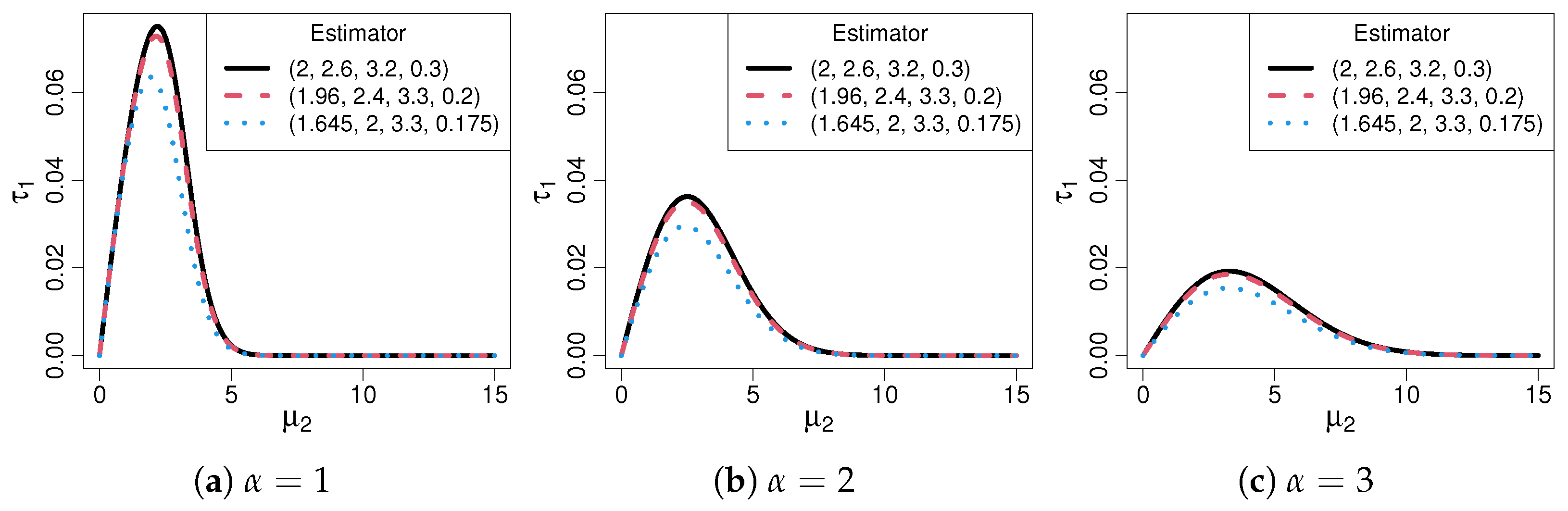
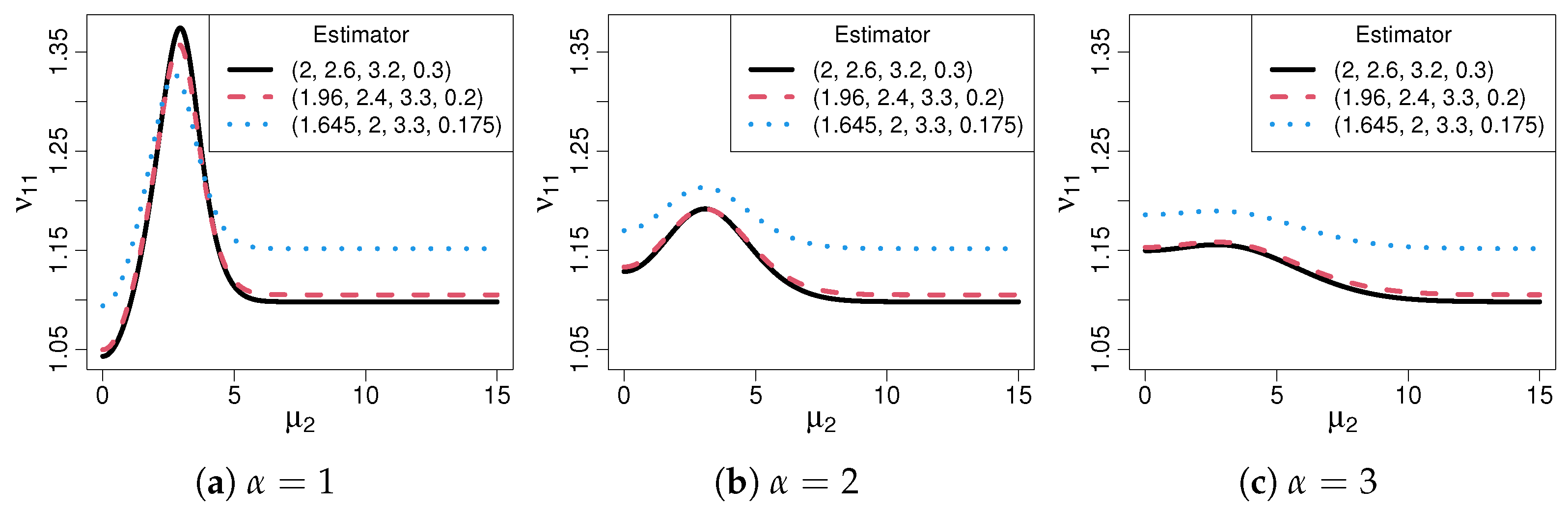
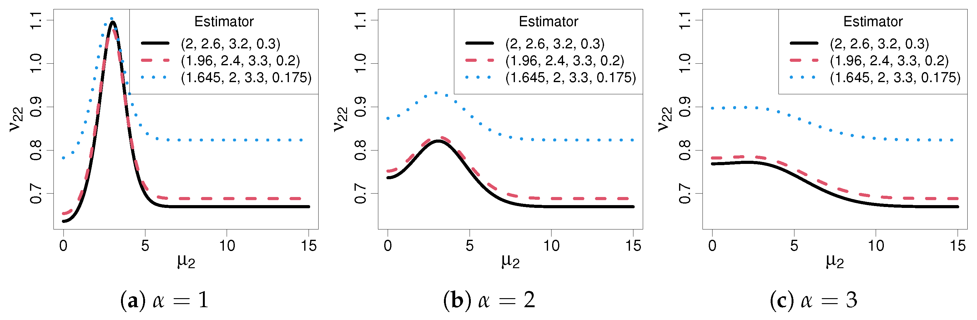
3.2. Contaminated Distribution Asymptotics

We now consider the asymptotic value and variance of $\mathbf{T}\left[\psi ,G_0\right]$, the multivariate location and scale solution of (6) under the contaminated model (1). Setting $ϵ=0.05$, we simulate the case where around 5% of the data pollutes our otherwise standard normal distribution. We hold $\alpha \in \{1,2,3\}$ and allow ${\mu }_2$ to vary. Figure 6 and Figure 7 show the asymptotic values for location and scale, respectively, for the smoothed three-part with parameters as tabulated in Table 2.

Note that if $\alpha \approx 0$, Figure 6 and Figure 7 would resemble the IF and Figure 8 and Figure 9 would resemble the CVF for the respective estimators. Instead, we are interested in the effect of scattered contamination in the vicinity of ${\mu }_2$.

Clearly, if ${\mu }_2$ is non-zero and $ϵ>0$, the estimator, which is a solution of Equation (3), will be consistent to something other than ${\left(\mu ,\sigma \right)}^T={\left(0,1\right)}^T$. This leads to the asymptotic bias, as given by $\mathbf{T}[\psi ,G_0]-\mathbf{T}[\psi ,\Phi ]$. One can see that as scattered contamination moves beyond the $(c+\delta )\sigma$ rejection point, the estimates tend towards the true $\mu$ and $\sigma$.

Figure 10 illustrates the benefits of smoothing for higher levels of contamination. The smoothed three-part estimator with $a=2,b=2.6,c=3.3$ is compared with $\delta \in \left\{0,0.3\right\}$. Clearly, asymptotic variance rises sharply around ${\mu }_2\approx 3.6$; however, with smoothing, the peak is ≈75% lower, indicating that smoothing is particularly useful when a higher level of contamination may be present in the vicinity of the rejection point.

4. Conclusions

A smoothed three-part redescender is introduced, as a refinement of Hampel’s three-part estimators, with definitions based entirely upon piecewise polynomials. Smoothing is shown to yield a significant improvement in both change of variance sensitivity and asymptotic variance near the rejection point when the distribution has higher levels of asymmetric contamination. Additionally, the resultant functional is shown to be both weakly continuous and Fréchet differentiable in the neighbourhood of the normal distribution. Other robustness measures, including efficiency and asymptotic bias, are largely unchanged from the non-smoothed functions, indicating little-to-no downside to using the smoothed $\psi$-functions in place of the traditional non-smoothed variants. Anywhere an M-estimator for location and/or scale has been employed for statistical applications may be enhanced by using our approach.

References

1. Hampel, F.R. The influence curve and its role in robust estimation. J. Am. Stat. Assoc. 1974, 69, 383–393. [Google Scholar] [CrossRef]
2. Bednarski, T.; Zontek, S. Robust estimation of parameters in a mixed unbalanced model. Ann. Stat. 1996, 24, 1493–1510. [Google Scholar] [CrossRef]
3. Bachmaier, M. Consistency of completely outlier-adjusted simultaneous redescending M-estimators of location and scale. Adv. Stat. Anal. 2007, 91, 197–219. [Google Scholar] [CrossRef]
4. Huber, P.J.; Ronchetti, E.M. Robust Statistics, 2nd ed.; John Wiley & Sons: New York, NY, USA, 2009. [Google Scholar]
5. Hampel, F.R.; Ronchetti, E.M.; Rousseeuw, P.J.; Stahel, W.A. Robust Statistics, the Approach Based on Influence Functions; John Wiley & Sons: New York, NY, USA, 1986. [Google Scholar]
6. Clarke, B.R. Robustness Theory and Application; John Wiley & Sons: Hoboken, NJ, USA, 2018. [Google Scholar]
7. Andrews, D.F.; Bickel, P.J.; Hampel, F.R.; Huber, P.J.; Rogers, W.H.; Tukey, J.W. Robust Estimates of Location: Survey and Advances; Princeton University Press: Princeton, NJ, USA, 1972. [Google Scholar]
8. Huber, P.J. Robust estimation of a location parameter. Ann. Math. Statist. 1964, 35, 73–101. [Google Scholar] [CrossRef]
9. Huber, P.J. Robust regression: Asymptotics, conjectures and Monte Carlo. Ann. Statist. 1973, 1, 799–821. [Google Scholar] [CrossRef]
10. Huber, P.J. Robust Statistics, 1st ed.; John Wiley & Sons: New York, NY, USA, 1981. [Google Scholar]
11. Arachchige, C.N.P.G.; Prendergast, L.A. Confidence intervals for median absolute deviations. Commun. Stat. Simul. Comput. 2024, 52, 1–10. [Google Scholar] [CrossRef]
12. Clarke, B.R.; Milne, C.J. A small sample bias correction and implications for inference. In Proceedings of the 59th ISI World Statistics Congress, Hong Kong, China, 25–30 August 2013. [Google Scholar]
13. Hearn, D.; Baker, M.P. Computer Graphics, 2nd ed.; Prentice Hall, Inc.: New York, NY, USA, 1997. [Google Scholar]
14. Rousseeuw, P.J.; Croux, C. Alternatives to the median absolute deviation. J. Am. Stat. Assoc. 1993, 88, 1273–1283. [Google Scholar] [CrossRef]
15. Hampel, F.R. Contributions to the Theory Of Robust Estimation. Ph.D. Thesis, University of California, Berkeley, CA, USA, 1968. [Google Scholar]
16. Huber, P.J. Robust Statistical Procedures, 2nd ed.; CBMS-NSF Regional Conference Series in Applied Mathematics; Society for Industrial and Applied Mathematics: Philadelphia, PA, USA, 1996. [Google Scholar]
17. Bednarski, T. Fréchet differentiability and robust estimation. In Asymptotic Statistics, Proceedings of the Fifth Prague Symposium 1994; Mandl, P., Hušková, M., Eds.; Springer: Berlin/Heidelberg, Germany, 1993; pp. 49–58. [Google Scholar]
18. Hampel, F.R. A general qualitative definition of robustness. Ann. Math. Statist. 1971, 42, 1887–1896. [Google Scholar] [CrossRef]
19. Clarke, B.R. Nonsmooth analysis and Fréchet differentiability of M-functionals. Probab. Theory Relat. Fields 1986, 73, 197–209. [Google Scholar] [CrossRef]
20. Varadarajan, V.S. On the convergence of probability distributions. Sankhy A 1958, 19, 23–26. [Google Scholar]
21. Prohorov, Y.V. Convergence of random processes and limit theorems in probability. Theory Probab. Appl. 1956, 1, 157–214. [Google Scholar] [CrossRef]
22. Rousseeuw, P.J. A new infinitesimal approach to robust estimation. Z. Wahrsch. Verw. Geb. 1981, 56, 127–132. [Google Scholar] [CrossRef]
23. Rousseeuw, P. New Infinitesimal Methods in Robust Statistics. Ph.D. Thesis, Vrije Universiteit Brussel, Brussells, Belgium, 1981. [Google Scholar]
Figure 1. Plots of the three-part redescenders.
Stats 08 00033 g001
Figure 2. Plot of the smoothed ψ 1 ; a , b , c , δ redescender for location.
Stats 08 00033 g002
Figure 3. Plot of the smoothed ψ 2 ; a , b , c , δ redescender for scale.
Stats 08 00033 g003
Figure 4. The CVF ( x ; ψ , Φ ) of the three-part ψ -function, with a = 1.96 , b = 2.4 , c = 3.3 , shown with and without δ = 0.2 smoothing.
Stats 08 00033 g004
Figure 5. The smoothed three-part CVF ( x ; ψ , Φ ) with smoothed functional parameters, as described in Table 2.
Stats 08 00033 g005
Figure 6. Plots of the asymptotic location solution of (6), τ 1 , for the estimators at (1) on μ 2 [ 0 , 15 ] . ϵ = 0.05 , representing an increasing scatter for the contaminating process. Smoothed ψ -function parameters are as described for Table 2.
Stats 08 00033 g006
Figure 7. Plots of the asymptotic scale solution of (6), τ 2 , for the estimators at (1) on μ 2 [ 0 , 15 ] . ϵ = 0.05 , representing an increasing scatter for the contaminating process. Smoothed ψ -function parameters are as described for Table 2.
Stats 08 00033 g007
Figure 8. Plots of asymptotic variance for the location solution of (6), labelled ν 11 , for the estimators at (1) on μ 2 [ 0 , 15 ] . ϵ = 0.05 , representing an increasing scatter for the contaminating process. Smoothed ψ -function parameters are as described for Table 2.
Stats 08 00033 g008
Figure 9. Plots’ asymptotic variance for the scale solution of (6), labelled ν 22 , for the estimators at (1) on μ 2 [ 0 , 15 ] . ϵ = 0.05 , representing an increasing scatter for the contaminating process. Smoothed ψ -function parameters are as described for Table 2.
Stats 08 00033 g009
Figure 10. Asymptotic variance on μ 2 [ 0 , 15 ] with ϵ = 0.15 and α = 1 . The functional parameters are a = 2 , b = 2.6 , c = 3.2 , and δ = 0 versus δ = 0.3 .
Stats 08 00033 g010