
Estimation of Weighted Extropy Under the α-Mixing Dependence Condition
 ,
,  and
and 
Abstract
1. Introduction
1.1. Definitions of Extropy and Its Extensions
1.2. Applications and Estimation Context
2. Non-Parametric Estimation of Weighted Extropy Under -Mixing Dependence
Recursive Estimator for Weighted Extropy
3. Recursive and Asymptotic Properties
4. Numerical Illustration
4.1. Simulation
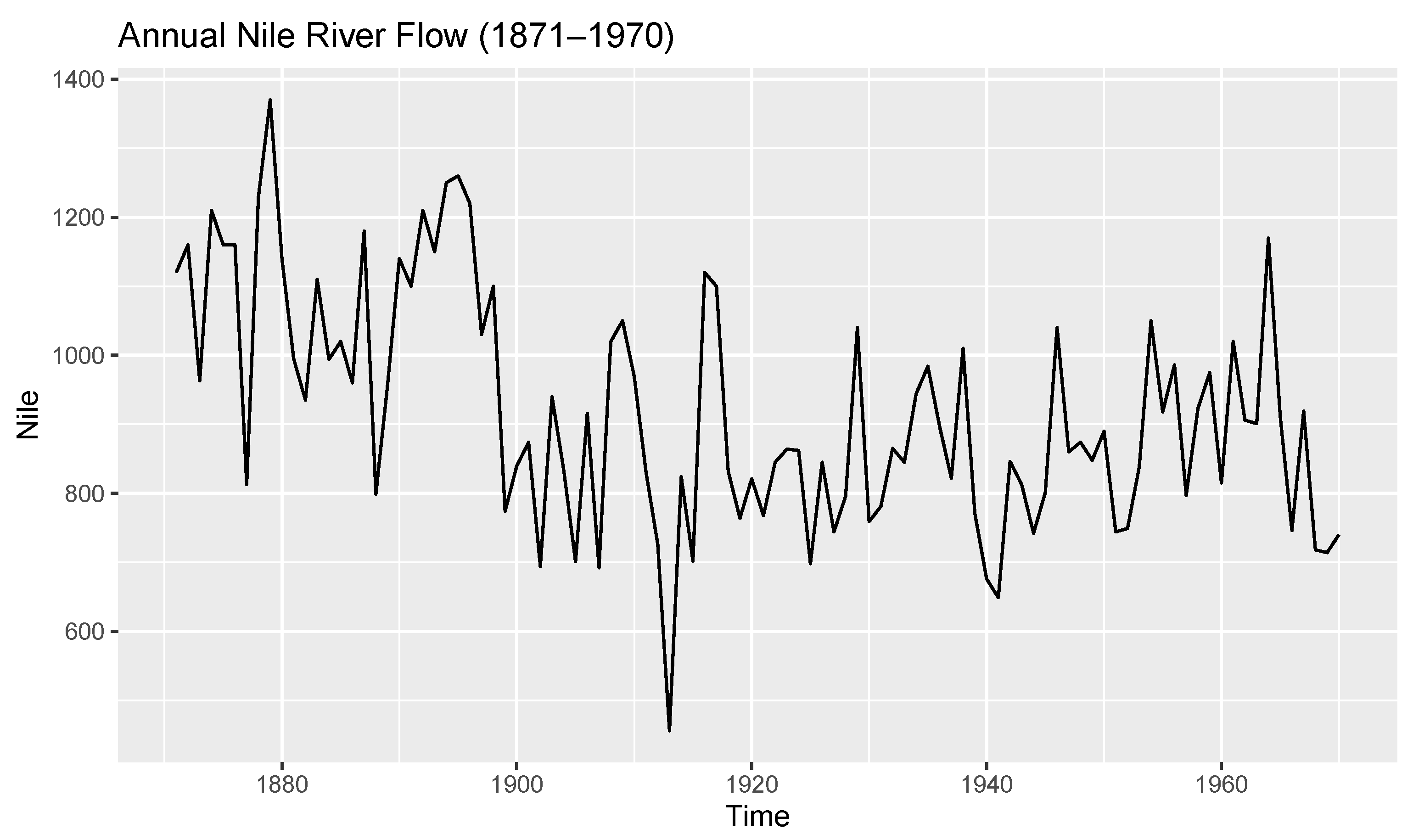
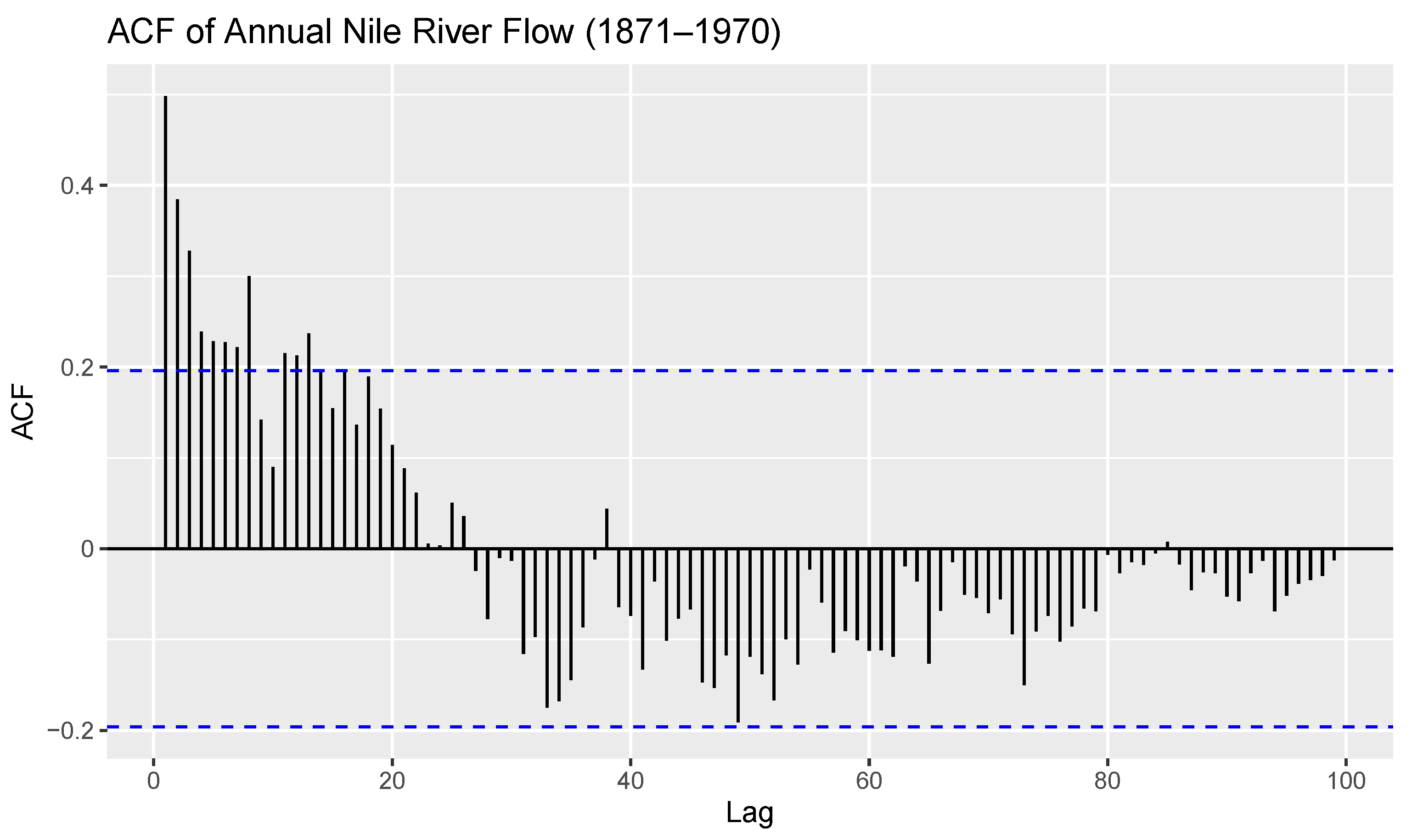
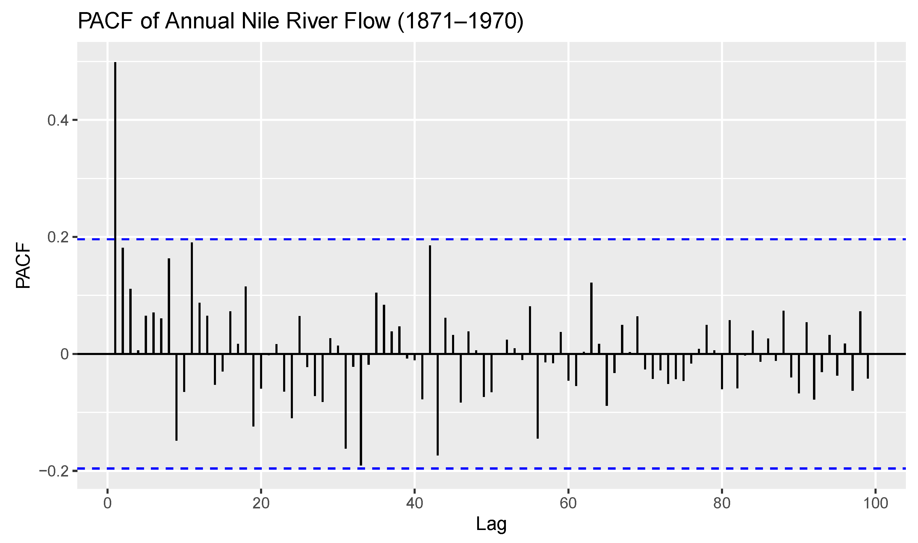
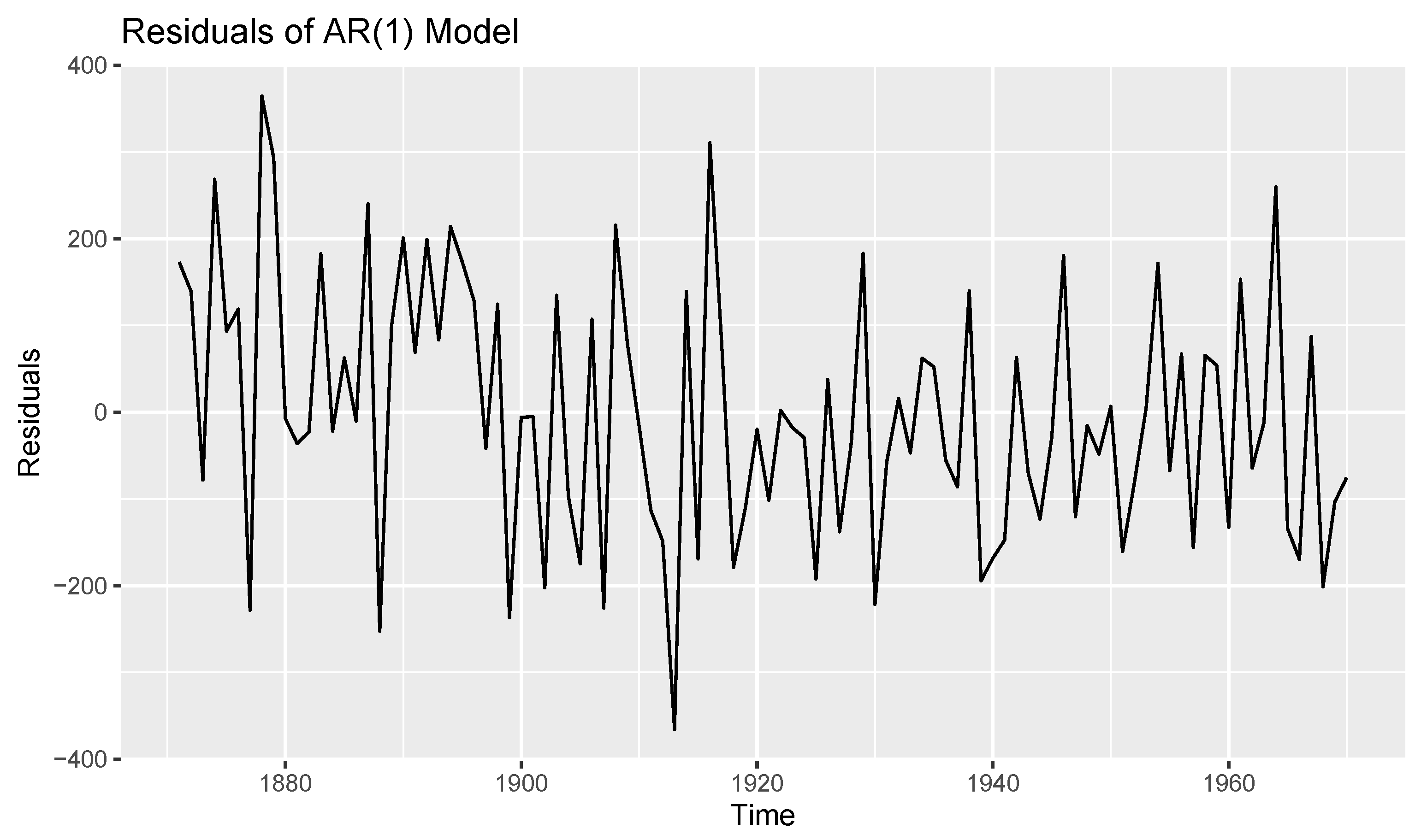
4.2. Data Analysis
- Data 1
- Data 2
5. Conclusions
Author Contributions
Funding
Institutional Review Board Statement
Informed Consent Statement
Data Availability Statement
Acknowledgments
Conflicts of Interest
References
- Shannon, C.E. A mathematical theory of communication. Bell System Tech. J. 1948, 27, 379–423. [Google Scholar] [CrossRef]
- Baratpour, S.; Ahmadi, J.; Arghami, N.R. Some characterizations based on entropy of order statistics and record values. Commun. Stat.-Theory Methods 2007, 36, 47–57. [Google Scholar] [CrossRef]
- Cover, T.M.; Thomas, J.A. Elements of Information Theory, 2nd ed.; John Wiley and Sons Inc.: Hoboken, NY, USA, 2006. [Google Scholar]
- Lad, F.; Sanfilippo, G.; Agro, G. Completing the logarithmic scoring rule for assessing probability distributions. Aip Conf. Proc. 2012, 1490, 13–30. [Google Scholar]
- Lad, F.; Sanfilippo, G.; Agro, G. Extropy: Complementary dual of entropy. Stat. Sci. 2015, 30, 40–58. [Google Scholar] [CrossRef]
- Qiu, G. Extropy of order statistics and record values. Stat. Probab. Lett. 2017, 120, 52–60. [Google Scholar] [CrossRef]
- Ebrahimi, N. How to measure uncertainty in the residual life time distribution. Sankhyā Indian J. Stat. Ser. A 1996, 58, 48–56. Available online: http://www.jstor.org/stable/25051082 (accessed on 24 April 2025).
- Qiu, G.; Jia, K. The residual extropy of order statistics. Stat. Probab. Lett. 2018, 133, 15–22. [Google Scholar] [CrossRef]
- Kamari, O.; Buono, F. On extropy of past lifetime distribution. Ric. Mat. 2020, 70, 505–515. [Google Scholar] [CrossRef]
- Krishnan, A.S.; Sunoj, S.M.; Nair, N.U. Some reliability properties of extropy for residual and past lifetime random variables. J. Korean Stat. Soc. 2020, 49, 457–474. [Google Scholar] [CrossRef]
- Di Crescenzo, A.; Longobardi, M. On weighted residual and past entropies. Sci. Math. Jpn. 2006, 64, 255–266. [Google Scholar]
- Balakrishnan, N.; Buono, F.; Longobardi, M. On weighted extropies. Commun. Stat.-Theory Methods 2022, 51, 6250–6267. [Google Scholar] [CrossRef]
- Hashempour, M.; Kazemi, M.R.; Tahmasebi, S. On weighted cumulative residual extropy: Characterization, estimation and testing. J. Theor. Appl. Stat. 2022, 56, 681–698. [Google Scholar] [CrossRef]
- Kazemi, M.R.; Hashempour, M.; Longobardi, M. Weighted Cumulative Past Extropy and Its Inference. Entropy 2022, 24, 1444. [Google Scholar] [CrossRef] [PubMed]
- Becerra, A.; de la Rosa, J.I.; Gonzalez, E.; Pedroza, A.D.; Escalante, N.I. Training deep neural networks with non-uniform frame-level cost function for automatic speech recognition. Multimed. Tools Appl. 2018, 77, 27231–27267. [Google Scholar] [CrossRef]
- Furuichi, S.; Mitroi, F.C. Mathematical inequalities for some divergences. Phys. Stat. Mech. Its Appl. 2012, 391, 388–400. [Google Scholar] [CrossRef]
- Martinas, K.; Frankowicz, M. Extropy-reformulation of the Entropy Principle. Period. Polytech. Chem. Eng. 2000, 44, 29–38. [Google Scholar]
- Vontobel, P.O. The Bethe permanent of a non-negative matrix. IEEE Trans. Inf. Theory 2012, 59, 1866–1901. [Google Scholar] [CrossRef]
- Qiu, G.; Wang, L.; Wang, X. On extropy properties of mixed systems. Probab. Eng. Inform. Sci. 2019, 33, 471–486. [Google Scholar] [CrossRef]
- Qiu, G.; Jia, K. Extropy estimators with applications in testing uniformity. J. Nonparametric Stat. 2018, 30, 182–196. [Google Scholar] [CrossRef]
- Hazeb, R.; Raqab, M.Z.; Bayoud, H.A. Non-parametric estimation of the extropy and the entropy measures based on progressive type-II censored data with testing uniformity. J. Stat. Comput. Simul. 2021, 91, 2178–2210. [Google Scholar] [CrossRef]
- Irshad, M.R.; Maya, R. Non-parametric log kernel estimation of extropy function. Chil. J. Stat. 2022, 13, 155–163. [Google Scholar]
- Irshad, M.R.; Archana, K.; Maya, R.; Longobardi, M. Estimation of Weighted Extropy with Focus on Its Use in Reliability Modeling. Entropy 2024, 26, 160. [Google Scholar] [CrossRef]
- Irshad, M.R.; Maya, R. Non-parametric estimation of past extropy under α-mixing dependence. Ric. Mat. 2022, 71, 723–734. [Google Scholar] [CrossRef]
- Maya, R.; Irshad, M.R.; Archana, K. Recursive and non-recursive kernel estimation of negative cumulative residual extropy under α-mixing dependence condition. Ric. Mat. 2023, 72, 119–139. [Google Scholar] [CrossRef]
- Maya, R.; Irshad, M.R.; Bakouch, H.; Krishnakumar, A.; Qarmalah, N. Kernel Estimation of the Extropy Function under α-Mixing Dependent Data. Symmetry 2023, 15, 796. [Google Scholar] [CrossRef]
- Wolverton, C.; Wagner, T. Asymptotically optimal discriminant functions for pattern classification. IEEE Trans. Inf. Theory 1969, 15, 258–265. [Google Scholar] [CrossRef]
- Masry, E. Recursive probability density estimation for weakly dependent stationary processes. IEEE Trans. Inf. Theory 1986, 32, 254–267. [Google Scholar] [CrossRef]
- Härdle, W.K. Smoothing Techniques: With Implementation in S; Springer Science and Business Media: Berlin/Heidelberg, Germany, 1991. [Google Scholar]
- Epanechnikov, V.A. Non-Parametric Estimation of a Multivariate Probability Density. Theory Probab. Its Appl. 1969, 14, 153–158. [Google Scholar] [CrossRef]
- Parzen, E. On estimation of a probability density function and mode. Ann. Math. Stat. 1962, 33, 1065–1076. [Google Scholar] [CrossRef]
- Wang, F.K. A new model with bathtub-shaped failure rate using an additive Burr XII distribution. Reliab. Eng. Syst. Saf. 2000, 70, 305–312. [Google Scholar]

| m | |||||||||
|---|---|---|---|---|---|---|---|---|---|
| () | () | ||||||||
| 50 | −0.0672 | 0.0578 | 0.0034 | −0.05447 | 0.07053 | 0.00499 | −0.05033 | 0.07467 | 0.00558 |
| ine 100 | −0.0768 | 0.0482 | 0.0024 | −0.05455 | 0.07045 | 0.00497 | −0.05037 | 0.07463 | 0.00557 |
| 150 | −0.0824 | 0.0426 | 0.0019 | −0.05476 | 0.07024 | 0.00494 | −0.05038 | 0.07462 | 0.00556 |
| 200 | −0.0866 | 0.0384 | 0.0015 | −0.05474 | 0.07026 | 0.00494 | −0.05039 | 0.07461 | 0.00551 |
| 250 | −0.0897 | 0.0353 | 0.0013 | −0.05473 | 0.07027 | 0.00494 | −0.05043 | 0.07457 | 0.00507 |
| 300 | −0.0924 | 0.0326 | 0.0011 | −0.05475 | 0.07025 | 0.00494 | −0.05044 | 0.07456 | 0.00481 |
| 350 | −0.0943 | 0.0307 | 0.0010 | −0.05479 | 0.07021 | 0.00493 | −0.05046 | 0.07454 | 0.00480 |
| 400 | −0.0963 | 0.0287 | 0.0009 | −0.05474 | 0.07026 | 0.00494 | −0.05047 | 0.07453 | 0.00476 |
| 450 | −0.0977 | 0.0273 | 0.0008 | −0.05473 | 0.07027 | 0.00494 | −0.05049 | 0.07451 | 0.00475 |
| 500 | −0.0989 | 0.0261 | 0.0007 | −0.05476 | 0.07024 | 0.00494 | −0.05049 | 0.07450 | 0.00475 |
| m | |||||||||
|---|---|---|---|---|---|---|---|---|---|
| () | () | ||||||||
| 50 | −0.09138 | 0.03362 | 0.00131 | −0.07475 | 0.05025 | 0.00257 | −0.06741 | 0.05759 | 0.00334 |
| 100 | −0.10085 | 0.02415 | 0.00073 | −0.07484 | 0.05016 | 0.00253 | −0.06749 | 0.05751 | 0.00332 |
| 150 | −0.10487 | 0.02013 | 0.00051 | −0.07492 | 0.05008 | 0.00251 | −0.06765 | 0.05735 | 0.00331 |
| 200 | −0.10734 | 0.01766 | 0.00040 | −0.07493 | 0.05007 | 0.00250 | −0.06760 | 0.05740 | 0.00331 |
| 250 | −0.11009 | 0.01491 | 0.00029 | −0.07495 | 0.05005 | 0.00250 | −0.06758 | 0.05742 | 0.00330 |
| 300 | −0.11160 | 0.01340 | 0.00025 | −0.07497 | 0.05003 | 0.00249 | −0.06762 | 0.05738 | 0.00330 |
| 350 | −0.11236 | 0.01264 | 0.00021 | −0.07502 | 0.04998 | 0.00248 | −0.06763 | 0.05737 | 0.00329 |
| 400 | −0.11342 | 0.01158 | 0.00019 | −0.07509 | 0.04991 | 0.00248 | −0.06765 | 0.05735 | 0.00329 |
| 450 | −0.11443 | 0.01057 | 0.00016 | −0.07512 | 0.04989 | 0.00247 | −0.06770 | 0.05730 | 0.00329 |
| 500 | −0.11466 | 0.01034 | 0.00015 | −0.07511 | 0.04989 | 0.00246 | −0.06775 | 0.05725 | 0.00328 |
| m | |||||||||
|---|---|---|---|---|---|---|---|---|---|
| () | () | ||||||||
| 50 | −0.03875 | 0.00832 | 0.000452 | −0.01078 | 0.01965 | 0.00039 | −0.00994 | 0.02059 | 0.00043 |
| 100 | −0.03318 | 0.00274 | 0.000155 | −0.01082 | 0.01962 | 0.00039 | −0.00988 | 0.02055 | 0.00043 |
| 150 | −0.02857 | 0.00187 | 0.000093 | −0.01092 | 0.01951 | 0.00039 | −0.01000 | 0.02043 | 0.00042 |
| 200 | −0.03167 | 0.00123 | 0.000061 | −0.01112 | 0.01932 | 0.00038 | −0.01025 | 0.02019 | 0.00042 |
| 250 | −0.02922 | 0.00121 | 0.000057 | −0.01121 | 0.01923 | 0.00038 | −0.01025 | 0.02018 | 0.00042 |
| 300 | −0.02939 | 0.00105 | 0.000044 | −0.01128 | 0.01915 | 0.00038 | −0.01026 | 0.02017 | 0.00041 |
| 350 | −0.02947 | 0.00096 | 0.000037 | −0.01172 | 0.01871 | 0.00037 | −0.01041 | 0.02003 | 0.00041 |
| 400 | −0.02995 | 0.00049 | 0.000035 | −0.01209 | 0.01834 | 0.00036 | −0.01065 | 0.01979 | 0.00041 |
| 450 | −0.02996 | 0.00048 | 0.000031 | −0.01249 | 0.01794 | 0.00036 | −0.01098 | 0.01946 | 0.00041 |
| 500 | −0.03024 | 0.00019 | 0.000028 | −0.01464 | 0.01580 | 0.00033 | −0.01180 | 0.01864 | 0.00040 |
| m | |||||||||
|---|---|---|---|---|---|---|---|---|---|
| () | () | ||||||||
| 50 | −0.03740 | 0.00697 | 0.000346 | −0.05136 | 0.02093 | 0.00104 | −0.01093 | 0.01951 | 0.00039 |
| 100 | −0.03283 | 0.00240 | 0.000136 | −0.04362 | 0.01318 | 0.00040 | −0.01095 | 0.01949 | 0.00039 |
| 150 | −0.03161 | 0.00118 | 0.000095 | −0.04096 | 0.01053 | 0.00026 | −0.01100 | 0.01943 | 0.00039 |
| 200 | −0.03146 | 0.00103 | 0.000063 | −0.03885 | 0.00842 | 0.00017 | −0.01129 | 0.01914 | 0.00038 |
| 250 | −0.03113 | 0.00070 | 0.000054 | −0.03789 | 0.00745 | 0.00013 | −0.01152 | 0.01892 | 0.00037 |
| 300 | −0.03111 | 0.00067 | 0.000044 | −0.03720 | 0.00676 | 0.00011 | −0.01172 | 0.01872 | 0.00036 |
| 350 | −0.03080 | 0.00037 | 0.000034 | −0.03684 | 0.00641 | 0.00009 | −0.01213 | 0.01831 | 0.00035 |
| 400 | −0.03072 | 0.00028 | 0.000032 | −0.03615 | 0.00572 | 0.00008 | −0.01231 | 0.01813 | 0.00035 |
| 450 | −0.03071 | 0.00028 | 0.000026 | −0.03552 | 0.00508 | 0.00007 | −0.01316 | 0.01728 | 0.00034 |
| 500 | −0.03040 | 0.00003 | 0.000025 | −0.03519 | 0.00475 | 0.00006 | −0.01478 | 0.01566 | 0.00033 |
| Estimator | Bias | ||
|---|---|---|---|
| −0.0343 | 0.0907 | 0.0104 | |
| −0.0216 | 0.1034 | 0.0115 |
Disclaimer/Publisher’s Note: The statements, opinions and data contained in all publications are solely those of the individual author(s) and contributor(s) and not of MDPI and/or the editor(s). MDPI and/or the editor(s) disclaim responsibility for any injury to people or property resulting from any ideas, methods, instructions or products referred to in the content. |
© 2025 by the authors. Licensee MDPI, Basel, Switzerland. This article is an open access article distributed under the terms and conditions of the Creative Commons Attribution (CC BY) license (https://creativecommons.org/licenses/by/4.0/).
Share and Cite
Maya, R.; Krishnakumar, A.; Irshad, M.R.; Chesneau, C. Estimation of Weighted Extropy Under the α-Mixing Dependence Condition. Stats 2025, 8, 34. https://doi.org/10.3390/stats8020034
Maya R, Krishnakumar A, Irshad MR, Chesneau C. Estimation of Weighted Extropy Under the α-Mixing Dependence Condition. Stats. 2025; 8(2):34. https://doi.org/10.3390/stats8020034
Chicago/Turabian StyleMaya, Radhakumari, Archana Krishnakumar, Muhammed Rasheed Irshad, and Christophe Chesneau. 2025. "Estimation of Weighted Extropy Under the α-Mixing Dependence Condition" Stats 8, no. 2: 34. https://doi.org/10.3390/stats8020034
APA StyleMaya, R., Krishnakumar, A., Irshad, M. R., & Chesneau, C. (2025). Estimation of Weighted Extropy Under the α-Mixing Dependence Condition. Stats, 8(2), 34. https://doi.org/10.3390/stats8020034